Comparative Study Using Neural Networks for 16S Ribosomal Gene Classification

Abstract

Bacterial 16S ribosomal gene was used to classify bacteria because it consists of both highly conservative region, as well as a hypervariable region, in its sequence. This hypervariable region serves as a discriminative factor to differentiate bacteria at taxonomic levels. In the past, many efforts have been made to correctly identify a bacterial species from environmental samples or human gut microbiome samples, yet this identification and subsequent classification task is challenging. For such bacterial taxonomic classification, several studies in the past have been performed based on k-mer frequency matching, assembly-based clustering, supervised/unsupervised machine learning models, and a very few studies with deep learning architectures. In this article, we study and propose six different deep learning architectures involving recurrent neural networks (RNNs) and convolutional neural networks to classify bacteria at a family, genus, and species taxonomic level using ∼12,900 16S ribosomal DNA sequences. The best classification accuracies achieved are 92%, 86%, and 70% at family, genus, and species taxonomic level, respectively, by variants of RNN.

1. Introduction

With the rise of refined, cheap, and effective sequencing technologies, it is possible to perform targeted sequencing for identification of bacteria obtained from different environmental samples (Achtman, 2002). Due to this phenomenon, a lot more sequencing projects/dataset have been submitted in National Center for Biotechnology Information (NCBI) database and have been made publicly available. Metagenomics studies have lately drawn a lot of attention since it doesn't require cell cultures to characterize bacterial species (Woo et al., 2008). Much more standardized approach is yet to be set for processing such large dataset without creating bias in these analyses. Currently bacterial taxonomic classification tasks depend on read-based sequence matching using tools like mothur and Quantitative Insights Into Microbial Ecology (QIIME) (Schloss et al., 2009; Caporaso et al., 2010). These tools perform matching of sequences using algorithms involving k-mer frequency, Basic Local Alignment Search Tool (BLAST), and suffix trees.

With rise of machine learning algorithms in past decade, various studies emerged involving naive Bayes approaches such as the Ribosomal Database Project (RDP) classifier, hierarchical clustering, random forests, and support vector machines (Wang et al., 2007; Zhang et al., 2008; Chaudhary et al., 2015; La Rosa et al., 2015; Fiannaca et al., 2018; Busia et al., 2019). To an extent all these studies rely on sequence similarity matching or k-mer frequency counting (Wang et al., 2007; Zhang et al., 2008; Chaudhary et al., 2015; La Rosa et al., 2015). Such k-mer based approaches can be limiting as they are independent of a motif position information along with initial sequencing errors/biases, which potentially creates noisy input data leading to an inaccurate analysis. With accessible computational resources and large public data repositories, deep learning techniques are in demand for classification tasks involving medical image analysis, cancer genomics, as well as correcting sequencing errors (Alipanahi et al., 2015; Park and Kellis, 2015).

There are various kinds of neural networks such as the convolutional neural networks (CNNs), the recurrent neural networks (RNNs), and simple deep neural networks. CNNs are generally considered to be a class of feed-forward artificial neural networks (ANNs), in which connections between nodes do not form a cycle and are trained to recognize patterns across the entire spatial domain. Whereas in RNNs, connections between nodes form a directed graph along a temporal sequence allowing this class of neural networks to exhibit temporal dynamic behavior, which is highly beneficial while processing sequences, for instance, time-series data. Thus, RNNs are trained to recognize patters over the time domain. CNNs are normally fixed input size architectures that have found most of their applications to be in the computer vision domain. However, recently scientific community has shown promising results for natural language processing (NLP) related classification tasks using CNNs. Some of the applications of such NLP related classification tasks involve sentiment analysis, spam detection, or topic categorization as CNNs can identify patterns (in form of n-grams) from regular expressions in any text data regardless of their position (Gao et al., 2014; Kim, 2014; Shen et al., 2014; Zeng et al., 2014; Johnson and Zhang, 2015; Nguyen and Grishman, 2015; Sun et al., 2015; Zhang and Wallace, 2015).

2. Dataset

The dataset was downloaded from Genomic-based 16S ribosomal RNA Database (GRD), which is a manually curated 16S ribosomal DNA sequence (Laboratory of Integrated Bioinformatics, 2015). The dataset has sequences that varies in lengths from 65 to 2900, which means that some of the sequences are not complete genes and some of the sequences have more base pairs than 16S rDNA sequence, which normally is ∼1500 bp long. The dataset has two separate files, one sequence fasta file and another metadata file containing tab-delaminated fasta header tag matched to bacterial taxonomy of which corresponding sequences belong to. This study focuses on bacterial classification at Family, Genus, and Species levels only since normally Phylum, Class, and Order level classification achieves >99% accuracy in most of the models due to sequences belonging to lesser categories (Fiannaca et al., 2018; Busia et al., 2019).

This dataset had sequences belonging to 272, 840, and 2456 categories for family, genus, and species level, respectively. For input files, each sequence was first separated with respective family, genus, and species category comma separated files. Each file was then further processed to cut each sequence in 100 bp nonoverlapping length to compare it with variable full-length sequences (results not included in this study). To ensure that each subsequence length is 100, if the last cut fragment is greater than 30 bp, it was then padded with Ns else the fragment was discarded. Ambiguous characters other than ATCG were treated as N for model characters. The sequences were randomly divided in 80% training and 20% testing (validation) dataset. This random split may cause an imbalance of classes in train versus test data; however, for our initial comparison, our approach was to proceed with minimizing the data-preprocessing tasks in deep learning.

3. Deep Learning Approach

Fiannaca et al. (2018) developed CNN based models for bacterial classification task. The CNN in its basic architectural form consists of convolutions and pooling operations. These operations generally lead to loss of sequence information related to data; for example, text data lose information about local order of words in a sentence. RNNs are popularly known as neural networks with memory and are designed to keep such orderly information intact, allowing the model to also learn the context (semantics). Thus, RNNs are a natural choice for sequence modeling applications, which have a time component, making them a powerful and preferred architecture for NLP applications. This work compares the performances of various neural networks for task at hand involving (1) three variants of RNNs, (2) two variants of CNNs, and (3) a combinational model, which makes use of the convolution and the recurrent layers.

In this study, all models are directly applied toward classification of DNA sequences without any prior feature engineering. Three different variations of RNN models, namely, vanilla RNN (model 1), long short-term memory (LSTM) (model 2), and bidirectional LSTM (BiLSTM) (model 3), as illustrated in Figure 1, and two different variations of CNN, namely, simple CNN (model 4) and multifilter (MF) CNN (model 5) along with a combinational model (model 6), were used to classify DNA sequence for achieving a higher classification accuracy. In this study, each category—family, genus, and species—was evaluated with all three aforementioned RNN and CNN variants trained on GRD dataset (Laboratory of Integrated Bioinformatics, 2015).

FIG. 1.

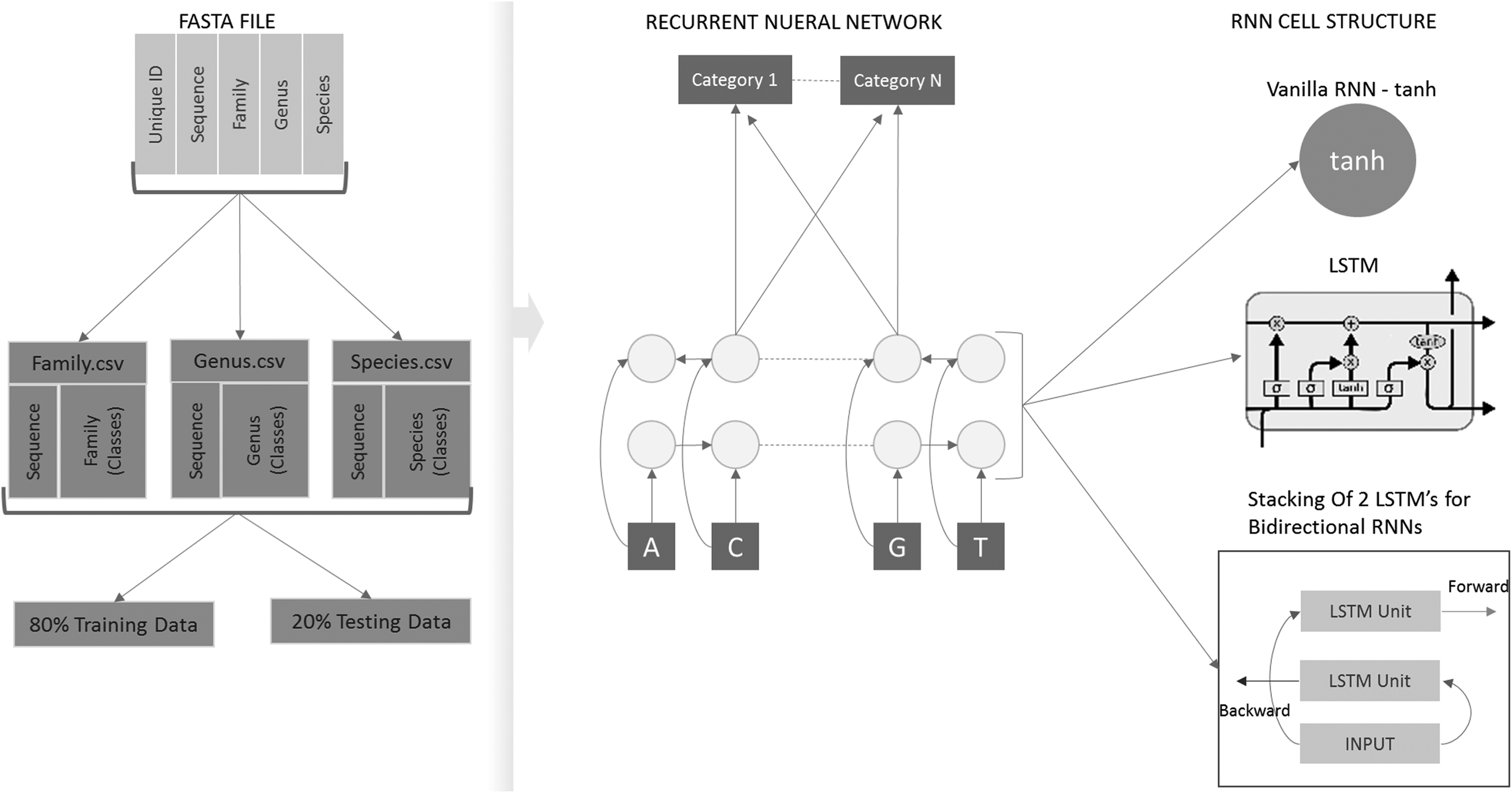
Overall architecture of data flow and RNN cell structures used in Model 1 (Vanilla RNN), Model 2 (LSTM) (Olah, 2015), and Model 3 (BiLSTM). LSTM, long short-term memory; BiLSTM, bidirectional LSTM; RNN, recurrent neural network.

DNA sequence classification can be modeled as a predictive modeling problem. For such problems, models generally take some sequence of inputs and predict a suitable category or class that better defines the sequence as an output. RNNs are an inherent choice of architecture for solving this problem primarily for two important reasons as follows: (1) because of the presence of internal memory and (2) their intrinsic ability to deal with variable length sequences as input. These neural networks are expected to take in variable length sequences as input and learn long-term dependencies between the various symbols of the input sequence, making them very suitable architectures for sequence classification, as well as sequence prediction tasks. In contrast, CNNs are known to be faster, that is, their computational times are shorter than RNNs. CNNs are a better architecture to extract features (feature detection tasks) compared to RNNs, which are intuitively suited for classification tasks involving a long range of semantic dependency (Yin et al., 2017). Therefore, both RNN models along with CNNs and combinational architecture are explored and used in this study.

3.1. Simple vanilla RNN

RNNs are known to be temporally deep networks, that is, the RNNs are usually unrolled or unfolded in time. Figure 2 is a simpler illustration of end-to-end RNN architectures of this study; furthermore, Sections 3.1 and 3.2 explain individual RNN cell structures denoted as recurrent layer 1/2/3 in Figure 2. There are certain formulas that govern the computations of the RNN. First, input x_t which is associated at time step t. Second, hidden state h_t or in other words the memory which is calculated by taking the previous hidden state [at the previous time step (t–1)] and present input into consideration, that is, h_t = f(Ux_t + Wh_t–1), where U,W are shared parameters associated with the different layers of RNN and f is a nonlinearity function, which is generally a tanh function or a rely function. Finally, output o_t was at time step t.

FIG. 2.

Illustration of the simplified model architecture where variable recurrent layer is dependent on RNN cell used.

The vanilla RNN cell unit is a simple unit where the previous hidden state h_t–1 and current input x_t are passed through the tanh nonlinearity function to update the current hidden state, that is, $h_{t} = \tanh W (_{h_{t - 1}}^{x_{t}}) .$

The drawback of vanilla RNNs is that it is difficult to train these networks. The updating of parameters for Vanilla RNNs happens the same way as that of ANNs, that is, through the back-propagation algorithm. The catch with respect to the calculation of gradients at every time step is with respect to that fact that vanilla RNNs have shared parameters between all-time steps of a layer, as opposed to independent parameters of an ANN. Thus, to calculate a gradient in a current time step there is a need to backpropagate to previous time steps until the present one making the vanilla RNN have difficulties in learning long-term dependencies, that is, dependencies between far away time steps. This backpropagation algorithm is called backpropagation through time, and this can lead to the vanishing/exploding gradient problem (Britz, 2015). Better variants of the RNNs like the LSTMs and the gated recurrent units (GRUs) have been designed to solve this problem, thus making these variants popular for tasks like sequence classification and prediction.

3.2. LSTM and bidirectional LSTM

More variants of RNNs were developed to address the shortcomings of a simple vanilla RNN. LSTMs are a popular variant of RNNs, each unit of the LSTM is associated with memory typically called a cell. In a LSTM cell unit, the memory is regulated with the help of three gates namely input gate $(i_{t})$ , output gate $(o_{t},$ hidden state $h_{t})$ , and forget gate $(f_{t})$ , which help determine which information needs to be added to the current cell state $(C_{t})$ and which information can be forgotten to update the cell state. The equation below represents the data flow from the current cell state, previous cell state, and the next state (Olah, 2015). $f_{t} = σ (W_{f} \cdot [h_{t - 1}, x_{t}] + b_{f})$

i_{t} = σ (W_{i} \cdot [h_{t - 1}, x_{t}] + b_{i})

{\tilde{C}}_{t} = tanh (W_{C} \cdot [h_{t - 1}, x_{t}] + b_{C})

C_{t} = f_{t} \times C_{t - 1} + i_{t} \times {\tilde{C}}_{t}

o_{t} = σ (W_{o} \cdot [h_{t - 1}, x_{t}] + b_{o})

h_{t} = o_{t} \times t a n h (C_{t})

The advantages of the LSTMs over vanilla RNNs are that they were specifically designed to overcome the vanishing gradient problems and are considered efficient in capturing long-term dependencies. Due to the vanishing gradient problem in Vanilla RNN models, LSTM was introduced because of its ability to update its own cell state. In LSTM unit (Fig. 1), the horizontal line on top acts as a “conveyer belt—with some minor linear interactions,” making backpropagation task much simpler (Olah, 2015).

Bidirectional LSTMs capture an idea; an output of recurrent unit at a particular time step not only depends on its past instances (past elements of the sequence) but also on the future instances. The idea of such a network is developed by stacking two layers of LSTMs over each other thus making an output dependent on the computation of hidden states from both LSTM layers as opposed to one in the unidirectional LSTM network.

3.3. CNN and MF CNN

CNNs or ConvNets are popular neural network models that gained prominence in the field of computer vision for their ability to have minimal preprocessing of data compared to other classification algorithms. In addition, they are able to eradicate the use of primitive hand engineered filters for singular instances of training data and maximize the usage of these neural networks to automatically learn the features from an image/video. ConvNets are generally used as good feature extractors that is successfully able to capture spatial/temporal dependencies of an image/video through the application of filters. Successive applications of these filters in the convolutional layers on any two-dimensional (2D)/three-dimensional (3D) data help in the reduction of size of the data by retaining all the critical features, which are important to make a final prediction. Recently, ConvNets have made a transition to NLP based applications. Instead of a 2D/3D convolutional layer, these applications rely on using one-dimensional convolutional layer. The filter size specified works as a sliding window that rolls over the entire sequence length, which is specified as a parameter in the convolutional layer.

Multifilter CNN was originally proposed by Kim, Yoon in Kim (2014). The filter size mentioned in the convolutional layer of the CNN defines the number of characters to consider in an iteration across the string of characters. The Multifilter CNN model in this study only includes different sized filters on the standard two convolutional layered model as illustrated in Figure 3. Such architectural changes allow the simple CNN model to integrate the different interpretations resulted from processing nucleotide sequence at different resolutions or different n-grams (groupings of characters with sliding window similar to k-mers) due to the variable filter sizes being used.

FIG. 3.

A model architecture depicting (A) MF CNN and (B) simple CNN. Global MaxPool layer in (B) serves as a flatten layer in this model. CNN, convolutional neural network.

3.4. Combinational model

In addition to aforementioned models, we compared RNN models with a combinational model for each category—family, genus, and species. This simple combinational model consists of one single layer of one-dimension convolution; one layer of pooling following with one layer of LSTM unit. These types of combinational models are highly used in text classification tasks, and they perform better than simple CNNs and MF CNN as they combine both the convolution and the recurrent layers in its architecture. This model is depicted in Figure 4 as below.

FIG. 4.

A model architecture depicting combinational model. Global MaxPool layer serves as a flatten layer in this model.

4. Results

For performance comparisons, each model was evaluated with same hyperparameter for family and genus level classification, whereas for species level classification, the model was run for longer number of epochs. Since the number of classes at species level is almost thrice higher than genus level, the complexity of classification also increases exponentially; hence, there is a stark difference in number of epochs hyperparameter. In addition, at species level only five to six sequences are present in certain classes, attributing to additional complexity in achieving better classification accuracies. Each of the below graphs shows the initial results which are comparable to other deep learning models, achieving >85% accuracies for both family and order and ∼70% accuracy for species level classification (Fiannaca et al., 2018; Busia et al., 2019). Figure 5 shows the loss and accuracies of each model for each taxonomic level.

FIG. 5.

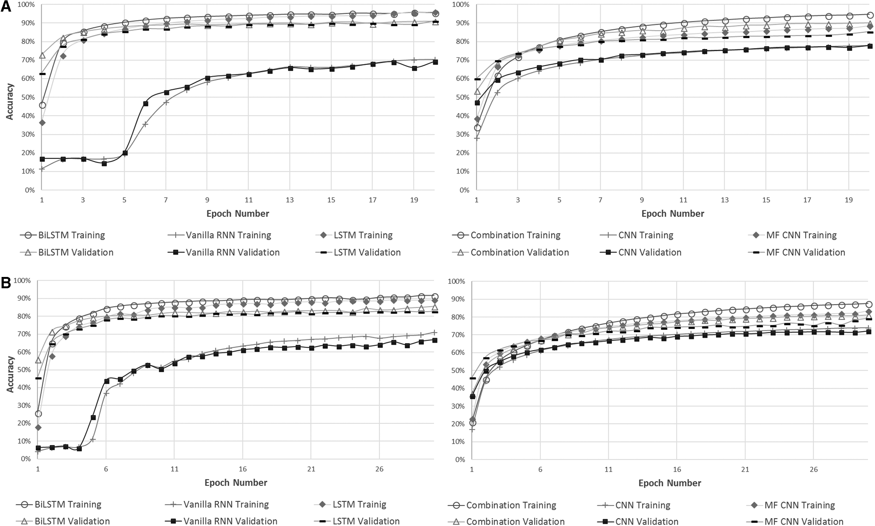
The training and validation(testing) accuracies of (A) family, (B) genus, and (C) species level classification for all six models.

The exact accuracies for family models were 90.85%, 91.24%, and 69.21%; for genus models were 85.63%, 82.92%, and 66.91%; and for species were 70.78%, 65.72%, and 37.7% achieved with BiLSTM, LSTM, and Vanilla RNN, respectively. At species level, model was stopped at 50 epochs since the accuracy was descending below 40%. The number of hidden units used in BiLSTM and LSTM models was 500, ran for 20 epochs with batch size of 200, with “adam” optimizer. The values for learning rate were 0.001, beta of 0.9, and decay of 0.0 for optimizer. The number of hidden units used in Vanilla RNN models was 500, ran for 100 epochs (model 2, 3) and for 20 epochs (model 1) with batch size of 200, with “adadelta” optimizer. The values for learning rate were 1.0, rho of 0.95, and decay of 0.0 for optimizer.

For the fixed input architecture models, that are CNNs, the accuracies achieved did not outperform the RNN models, especially BiLSTM (model 3) and LSTM (model 2). However, the interesting outcome observed was that combination model (model 6) surpassed the performance of MF CNN model (model 5), as well as simple CNN model (model 4), at all three taxonomic levels included in this study. Comparing the simplistic models from the two architecturally different networks, one can make a conclusion that simple CNN (model 4) outperformed Vanilla RNN (model 1) at all three taxonomic levels. All of the hyperparameters were exactly same as RNNs except for the optimizer, which was “adam” for all CNN models. Table 1 further elaborates the results achieved by all six models.

Table 1.

Final Accuracies and Losses of All Six Models for Each Family, Genus, and Species Taxonomic Levels

Model	Model name	Family		Genus		Species
Model	Model name	Validation loss	Validation accuracy (%)	Validation loss	Validation accuracy (%)	Validation loss	Validation accuracy (%)
1	Vanilla RNN	1.446	69.21	1.742	66.91	3.754^a	37.7^a
2	LSTM	0.328	91.24	0.933	82.92	1.762	65.72
3	BiLSTM	0.531	90.85	0.774	85.63	0.914	70.78
4	CNN	1.010	77.91	1.536	72.25	3.031	57.13
5	MF CNN	0.746	85.52	1.275	79.27	2.686	61.71
6	Combination	0.4742	90.00	1.010	81.11	2.659	63.01

Accuracies highlighted in bold are the highest classification accuracy achieved within each level.

Stopped at 50 epochs since this model's performance accuracy was dipping below 40%.

LSTM, long short-term memory; BiLSTM, bidirectional LSTM; CNN, convolutional neural network; MF, multifilter; RNN, recurrent neural network.

5. Conclusion and Future Work

The need of faster and accurate bacterial sequence classification is a critical task in analysis of metagenomics sequencing for gut microbiome and environmental samples. In recent years, the data repositories for such sequencing projects have been on the rise. The goal of this work was to perform detailed comparative analysis of various deep models and their performances. In general, species level sequences are categorized in almost three times more classes than genus and twelve times more classes than order; hence, the model performance reduces drastically compared to other levels. This is also because bacterial dataset is not balanced; data for some species are easily available than the rare species. Although stacking of deeper LSTM units sounds lucrative in terms of performance for RNNs, the hyperparameter optimization for such network can get difficult. BiLSTM models (model 3) achieved the highest accuracies for genus and species levels, whereas LSTM models (model 2) achieved the highest accuracy for family level among all the models studied. Considering all the CNN models, the combination model (model 6) achieved the highest accuracies at all levels.

This work doesn't provide a final tool for analysis of metagenomic samples, but rather serves as a study of possible classification architectures to be included in future endeavors. This work doesn't provide statistical makeup of each metagenomics sample, but provides a comparison of which deep models can be deployed for this classification task. In future, three approaches are being taken to improve accuracies separately and simultaneously: (1) compare our results using a larger dataset, as well as raw read dataset, (2) use full gene sequences instead of 100-bp length sequences to create an ensemble model, and (3) stricter data cleansing approaches even if few of the classes are lost. In all the machine learning and deep learning approaches for taxonomy classification task, the relationship of hierarchical data is oversimplified and, in most cases, ignored. In future we plan to incorporate these relationships to improve final accuracy at species level.

Footnotes

Author Disclosure Statement

The authors declare they have no conflicting financial interests.

Funding Information

Graduate Student, Heta P. Desai, was supported by Brains and Behavior (B&B) Fellowship program from Neuroscience Institute of Georgia State University. No other funding was received for this study.

References

Achtman

2002. A phylogenetic perspective on molecular epidemiology, 485–509. In Sussman M, ed. Molecular Medical Microbiology. Academic Press, London.

Alipanahi

, Delong

, Weirauch

M.T.

, et al. 2015. Predicting the sequence specificities of DNA-and RNA-binding proteins by deep learning. Nat. Biotechnol. 33, 831.

Britz

2015. Recurrent neural networks tutorial, Part 1–Introduction to RNNs. Available at: www.wildml.com/2015/09/recurrent-neural-networks-tutorial-part-1-introduction-to-rnns. Accessed January 20, 2018.

Busia

, Dahl

G.E.

, Fannjiang

, et al. 2019. A deep learning approach to pattern recognition for short DNA sequences. bioRxiv 353474.

Caporaso

J.G.

, Kuczynski

, Stombaugh

, et al. 2010. QIIME allows analysis of high-throughput community sequencing data. Nat. Methods, 7, 335.

Chaudhary

, Sharma

A.K.

, Agarwal

, et al. 2015. 16S classifier: A tool for fast and accurate taxonomic classification of 16S rRNA hypervariable regions in metagenomic datasets. PLoS One, 10, e0116106.

Fiannaca

, La Paglia

, La Rosa

, et al. 2018. Deep learning models for bacteria taxonomic classification of metagenomic data. BMC Bioinformatics, 19, 198.

Gao

, Pantel

, Gamon

, et al. 2014. Modeling interestingness with deep neural networks, 2–13. In Proceedings of the 2014 Conference on Empirical Methods in Natural Language Processing (EMNLP), Doha, Qatar.

Johnson

, and Zhang

2015. Effective use of word order for text categorization with convolutional neural networks (NAACL-2015). Association for Computational Linguistics, Denver, CO.

10.

Kim

2014. Convolutional neural networks for sentence classification, 1746–1751. In Proceedings of the 2014 Conference on Empirical Methods in Natural Language Processing (EMNLP 2014), Doha, Qatar.

11.

Laboratory for Integrated

Bioinformatics

, Center for Integrative Medical Sciences, RIKEN (2015). GRD—Genomic-based 16S ribosomal RNA database. Available at: https://metasystems.riken.jp/grd/about.html. Accessed November 1, 2018.

12.

La Rosa

, Fiannaca

, Rizzo

, et al. 2015. Probabilistic topic modeling for the analysis and classification of genomic sequences. BMC Bioinformatics, 16, S2.

13.

Nguyen

T.H.

, and Grishman

2015. Relation extraction: Perspective from convolutional neural networks, 39–48. Workshop on Vector Modeling for NLP. Association for Computational Linguistics, Denver, CO.

14.

Olah

(2015). Understanding lstm networks. Available at: https://colah.github.io/posts/2015-08-Understanding-LSTMs. Accessed March 1, 2018.

15.

Park

, and Kellis

2015. Deep learning for regulatory genomics. Nat. Biotechnol. 33, 825.

16.

Schloss

P.D.

, Westcott

S.L.

, Ryabin

, et al. 2009. Introducing mothur: Open-source, platform-independent, community-supported software for describing and comparing microbial communities. Appl. Environ. Microbiol. 75, 7537–7541.

17.

Shen

, He

, Gao

, et al. 2014. A latent semantic model with convolutional-pooling structure for information retrieval, 101–110. In Proceedings of the 23rd ACM International Conference on Conference on Information and Knowledge Management—CIKM’14, Shanghai, China.

18.

Sun

, Lin

, Tang

, et al. 2015. Modeling mention, context and entity with neural networks for entity disambiguation. Ijcai 1333–1339, Buenos Aires, Argentina.

19.

Wang

, Garrity

G.M.

, Tiedje

J.M.

, et al. 2007. Naive Bayesian classifier for rapid assignment of rRNA sequences into the new bacterial taxonomy. Appl. Environ. Microbiol. 73, 5261–5267.

20.

Woo

P.C.Y.

, Lau

S.K.P.

, Teng

J.L.L.

, et al. 2008. Then and now: Use of 16S rDNA gene sequencing for bacterial identification and discovery of novel bacteria in clinical microbiology laboratories. Clin Microbiol. Infect. 14, 908–934.

21.

Yin

, Kann

, Yu

, et al. 2017. Comparative study of CNN and RNN for natural language processing. arXiv preprint arXiv:1702.01923.

22.

Zeng

, Liu

, Lai

, et al. 2014. Relation classification via convolutional deep neural network. Proc. Coling 25, 2335–2344. Proceedings of COLING 2014, the 25th International Conference on Computational Linguistics: Technical Papers. Dublin, Ireland.

23.

Zhang

A.B.

, Sikes

D.S.

, Muster

, et al. 2008. Inferring species membership using DNA sequences with back-propagation neural networks. Syst. Biol. 57, 202–215.

24.

Zhang

, and Wallace

2015. A sensitivity analysis of (and practitioners' guide to) convolutional neural networks for sentence classification. 253–263. In Proceedings of the Eighth International Joint Conference on Natural Language Processing, Vol. 1: Long Papers. Asian Federation of Natural Language Processing, Taipei, Taiwan.