
Abstract
1. Introduction
Different tissues of the body have different cellular compositions. The composition of tumor tissue is different from that of normal tissue. Also, when comparing two tumor tissues, their cellular composition can differ greatly. The relatively small populations of tumor-infiltrating immune cells are of particular importance. They affect progression of disease (Galon et al., 2006) and success of treatment (Fridman et al., 2012). Immune therapies block communication lines between tumor cells and infiltrating immune cells. Whether they are successful or not depends on the presence, quantity, and molecular subtype of the infiltrating immune cells (Hackl et al., 2016). Immune cell populations are typically small, and their molecular phenotype can be difficult to observe under the microscope. Single-cell technologies such as fluorescence-activated cell sorting (FACS; e.g., [Ibrahim and van den Engh, 2007]), cytometry by time-of-flight (Bendall et al., 2011), and single-cell RNA sequencing (Wu et al., 2014) assess molecular features on the single-cell level and can thus be used to determine the cellular tissue composition experimentally.
A more cost- and work-efficient alternative to single-cell assays is a combination of bulk tissue gene expression profiling with digital tissue deconvolution (DTD) (Lu et al., 2003; Abbas et al., 2009; Gong et al., 2011; Qiao et al., 2012; Altboum et al., 2014; Newman et al., 2015; Li et al., 2016). DTD addresses the following inverse problem: given the bulk gene expression profile y of a tissue, what is the cellular composition c of that tissue? Supervised DTD assumes that there is a matrix X whose columns are reference profiles of individual cell types. The composition c of y can be computed by minimizing
The practical objective of DTD is to estimate c correctly, whereas the formal objective of common DTD algorithms is to estimate y correctly. If tissue expression profiles were exact mixtures of reference profiles, existing methods should work perfectly. They are not and this causes problems:
Collections of reference profiles can be incomplete. There might be cells in the tissue that are not represented by the reference profiles. In that case the global DTD problem is not solvable, and DTD algorithms will compensate for the contributions of these cells by increasing the frequencies of other cell types. Small cell fractions are hard to quantify. From a practical point of view, this is probably the most important point, and improvements are needed badly. Immunological cell populations in a tumor are small, but they may determine the reaction of a tumor to immunotherapy. Therefore, DTD algorithms must use faint signals from small cell populations more effectively. Some cell types can hardly be distinguished by their expression profiles. The profile of an epithelial cell differs greatly from that of a lymphoid cell. For two immunological subentities of CD8+ T cells, the differences are more subtle. The more similar two cell types are, the more similar are their expression profiles, and the more difficult is their distinction.
In summary, different applications need different approaches. One way to adapt the estimation of c is to adapt the loss function
2. Methods
2.1. Notations
Let
2.2. Loss-function learning
Following the established linear DTD algorithms, we approximate the mixture
where
In contrast to standard DTD algorithms, which determine g by prior knowledge or separate statistical analysis, we learn g directly from data. To this end, we assume that we have a training set of mixtures
Our method has two nested objective functions: an outer function
where the
The minimum of
with
with
where
Using these equations, we implemented our optimization algorithm. For a more efficient implementation, consider section 5.2. Constraints
3. Results
3.1. DTD of melanomas
For both training and validation, we need expression profiles of cellular mixtures of known composition. We used expression data of melanomas whose composition has been experimentally resolved using single-cell RNAseq profiling (Tirosh et al., 2016). These data included 4645 single-cell profiles from 19 melanomas. The cells were annotated as T cells (2068), B cells (515), macrophages (126), endothelial cells (65), cancer-associated fibroblasts (CAFs) (61), natural killer (NK) cells (52), and tumor/unclassified (1758). The first 9 melanomas defined our validation cohort and the remaining 10 defined our training data.
First, data were transformed into transcripts per million. Then, for each cell cluster we sampled
The sum of all single-cell profiles of a melanoma gave us bulk profiles. In addition, we generated a large number of artificial bulk profiles by randomly sampling single-cell profiles and summing them up. All bulk profiles were normalized to the same number of reads as those in
3.2. Loss-function learning improves DTD accuracy in the case of incomplete reference data
We generated 2000 artificial cellular mixtures from our training cohort. For each of these mixtures, we randomly drew 100 single-cell profiles, summed up their raw counts, and normalized them to a fixed number of total counts. Analogously, we generated 1000 artificial cellular validation mixtures.
Then, we restricted X to three cell types (T cells, B cells, and macrophages). Hence endothelial cells, CAFs, NK cells, and tumor/unclassified cells in the mixtures are not represented in X. For standard DTD with
To test the limits of the approach, we excluded all but the macrophages, which account for <

Deconvolution performance with only a single reference profile (macrophages). Predicted cell frequencies are plotted versus real frequencies. Results from the standard DTD model with
3.3. Loss-function learning improves the quantification of small cell populations
We generated data as above for mixtures of T cells, B cells, macrophages, endothelial cells, CAFs, NK cells, and tumor/unclassified cells, and use all cells except the tumor cells in X. This time we control the abundance of B cells in the simulated mixtures at 0–5 cells, 5–15, 15–30, 30–50, and 50–75 out of 100 cells. Not surprisingly, small fractions of B cells were harder to quantify than large fractions. Loss-function learning improved the accuracy for all amounts of B cells, but the improvements were greatest for small amounts (Fig. 2a). With only 0–5 cells in a mixture, the accuracy improved from
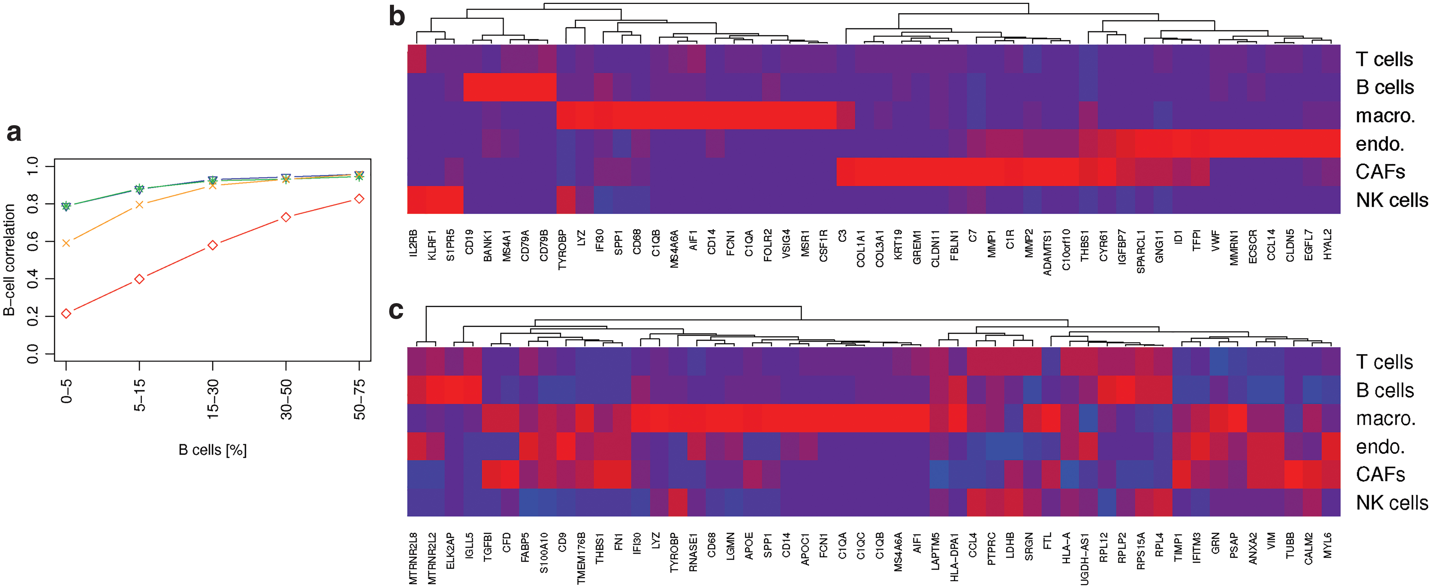
Plot
If we compare the top-ranked genes of the model learned for the small B cell population (Fig. 2b) with that of the macrophage-focused simulation (Fig. 2c), we observe that the former still comprises marker genes to distinguish all cell types, whereas the latter focuses on genes that characterize macrophages.
3.4. Loss-function learning improves the distinction of closely related cell types
The cell types that were annotated by Tirosh et al. (2016) displayed very different expression profiles. If we are interested in T cell subtypes such as CD8+ T cells, CD4+ T-helper (Th) cells, and regulatory T cells (Tregs), reference profiles are more similar and DTD is more challenging. We subdivided the fraction of annotated T cell profiles as follows: all T cells with positive CD8 (sum of CD8A and CD8B) and zero CD4 count were labeled CD8+ T cells (1130). Vice versa, T cells with zero CD8 and positive CD4 count were labeled CD4+ T cells (527). These were further split into Tregs if both their FOXP3 and CD25 (IL2RA) count was positive (64), and CD4+ Th cells otherwise (463). T cells that fulfilled neither the CD4+ nor the CD8+ criteria (411) contributed to the mixtures, but were not assessed by DTD. We augmented the reference matrix X, here consisting of T cells, B cells, macrophages, endothelial cells, CAFs, and NK cells, by these cell types, replacing the original all T cell profile with the more specific profiles for CD8+ T cells, CD4+ Th, and Tregs. Then we simulated 2000 training and 1000 test mixtures as already described.
For standard DTD with
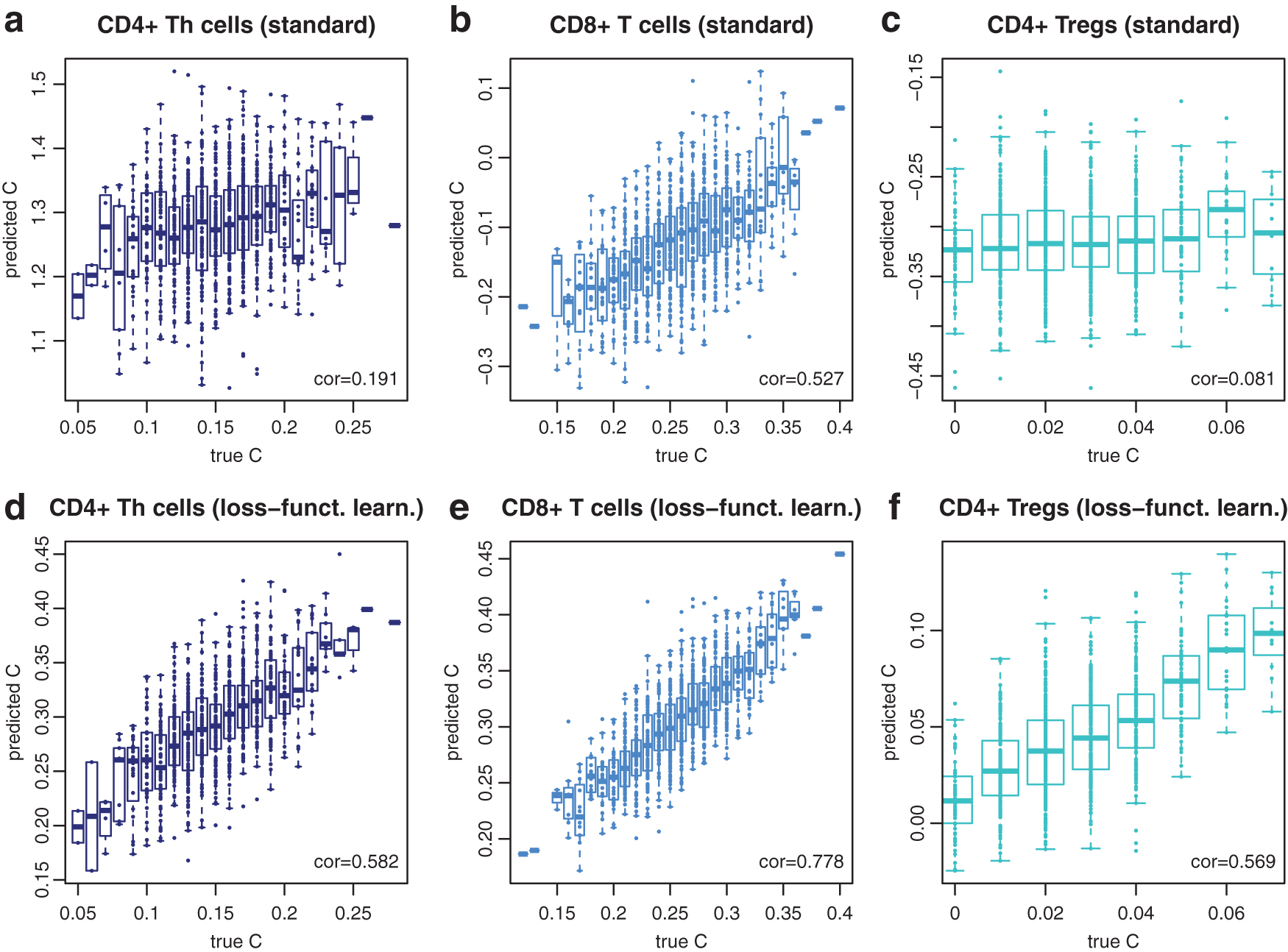
Deconvolution of T cell subentities. Results from the standard DTD model with
3.5. Loss-function learning is beneficial even for small training sets, and the performance improves as the training data set grows
We repeated the simulation in section 3.4, but varied the size of the training data set. We observed that loss-function learning improved accuracy for training data sets as small as 15 samples. Moreover, with more training data added, the boost in performance grew and saturated only for training sets with >1000 samples (Fig. 4).
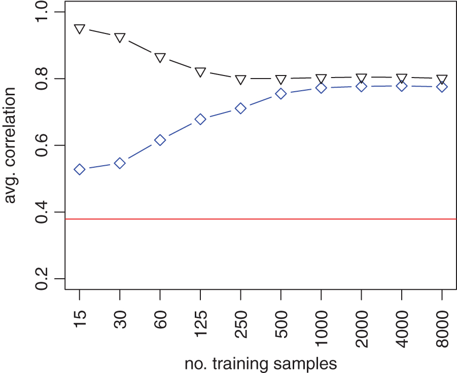
Performance with and without loss-function learning as a function of the size of the training set. Performance was assessed by calculating the average correlations between predicted and true cellular contributions over all cell types. The blue diamonds and black triangles correspond to the performance of loss-function learning for the validation mixtures and training mixtures, respectively. The performance of standard DTD with
3.6. High-performance computing-empowered loss-function learning rediscovers established cell markers and complements them by new discriminatory genes for improved performance
Here, we introduce a final model, optimized on the 5000 most variable genes. For this purpose, we generated 25,000 training mixtures from the melanomas of the training data. With standard desktop workstations, the solution of this problem was computationally not feasible. A single computation of the gradient took 16 hours (2x Intel Xeon CPU [X5650; Nehalem Six Core, 2.67 GHz], 148 Gb RAM), and this needs to be computed several hundred times until convergence. Therefore, we developed a high-performance computing implementation of our code by parallelizing Equations (3) and (6) with MPI, using the pbdMPI library (Chen et al., 2012a, 2012b) as an interface. Furthermore, we linked R with the Intel Math Kernel Library for threaded and vectorized matrix operations. We ran the algorithm on 25 nodes of our QPACE 3 machine Georg et al. (2017) with 8 MPI tasks per node and 32 hardware threads per task, where each thread can use two AVX512 vector units. In 16 hours, 5086 iterations were finished, after which the loss (3) was stable to within 1%.
The high-performance model includes several genes, whose expression is characteristic for the cells distinguished in this study. These include, among others, the CD8A gene, which encodes an integral membrane glycoprotein essential for the activation of cytotoxic T-lymphocytes (Veillette et al., 1988) and the protection of a subset of NK cells against lysis, thus enabling them in contrast to CD8− NK cells to lyse multiple target cells (Addison et al., 2005). As evident from Figure 5, NK cells are clearly set apart from all the other cell types studied by the expression of the killer cell lectin-like receptor genes KLRB1, KLRC1, and KLRF1 (Moretta et al., 2001). B cells, in contrast, are clearly characterized by the expression of (1) CD19, which assembles with the antigen receptor of B lymphocytes and influences B cell selection and differentiation (Rickert et al., 1995), (2) CD20 (MS4A1), which is coexpressed with CD19 and functions as a store-operated calcium channel (Li et al., 2003), (3) B lymphocyte kinase (BLK), a src-family protein tyrosine kinase that plays an important role in B cell receptor signaling and phosphorylates specifically (4) CD79A at Tyr-188 and Tyr-199 as well as CD79B (not among the top 150 genes) at Tyr-196 and Tyr-207, which are required for the surface expression and function of the B cell antigen receptor complex (Hsueh and Scheuermann, 2000), and (5) B Cell Linker (BLNK), which bridges BLK activation with downstream signaling pathways (Wienands et al., 1998). The expression of FOXP3 is also highly cell specific. FOXP3 distinguishes Tregs from other CD4+ cells and functions as a master regulator of their development and function (Hori et al., 2003). Finally, CD4+ Th cells are distinguished indirectly from all the other aforementioned lymphocytes by the lack of expression of cell type-specific genes.
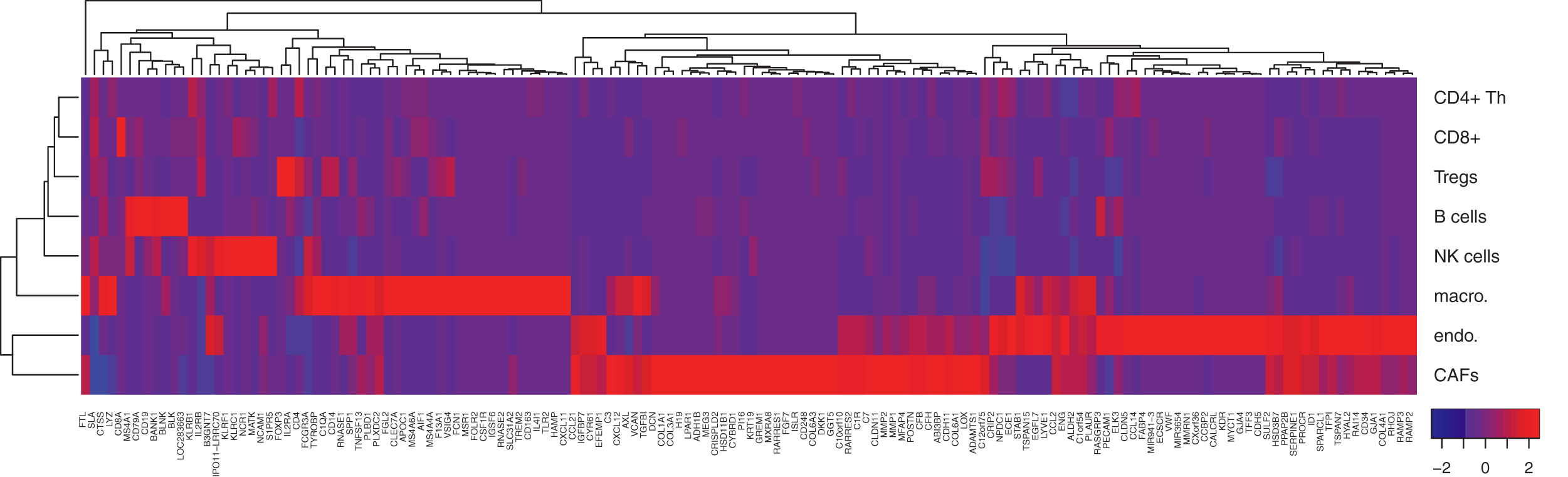
Heatmap of X for the features with the top 150 weights (
In contrast to lymphocytes, macrophages, CAFs, and endothelial cells, which line the interior surface of blood vessels and lymphatic vessels, are characterized each by a much larger number of genes. Exemplary genes include CD14, CD163, MSR1, STAB1, and CSF1R for macrophages. The monocyte differentiation antigen CD14, for instance, mediates the innate immune response to bacterial lipopolysaccharide by activating the NF-
Noteworthy is also GREM1, an antagonist of the bone morphogenetic protein pathway. Its expression and secretion by stromal cells in tumor tissues promote the survival and proliferation of cancer cells (Sneddon et al., 2006). Genes characteristic for endothelial cells include among others CDH5, a member of the cadherin superfamily essential for endothelial adherens junction assembly and maintenance (Gory-Faure et al., 1999), the endothelial cell-specific chemotaxis receptor (ECSCR) gene, which encodes a cell surface single-transmembrane domain glycoprotein that plays a role in endothelial cell migration, apoptosis and proliferation (Shi et al., 2011), claudin-5 (CLDN5), which forms the backbone of tight junction strands between endothelial cells (Haseloff et al., 2015), and the von Willebrand factor, which mediates the adhesion of platelets to sites of vascular damage by binding to specific platelet membrane glycoproteins and to constituents of exposed connective tissue (Sadler, 1998).
We discussed 28 genes of the top 150 shown in Figure 5. These genes have a total weight of 28% of all 5000 gene weights (calculated as
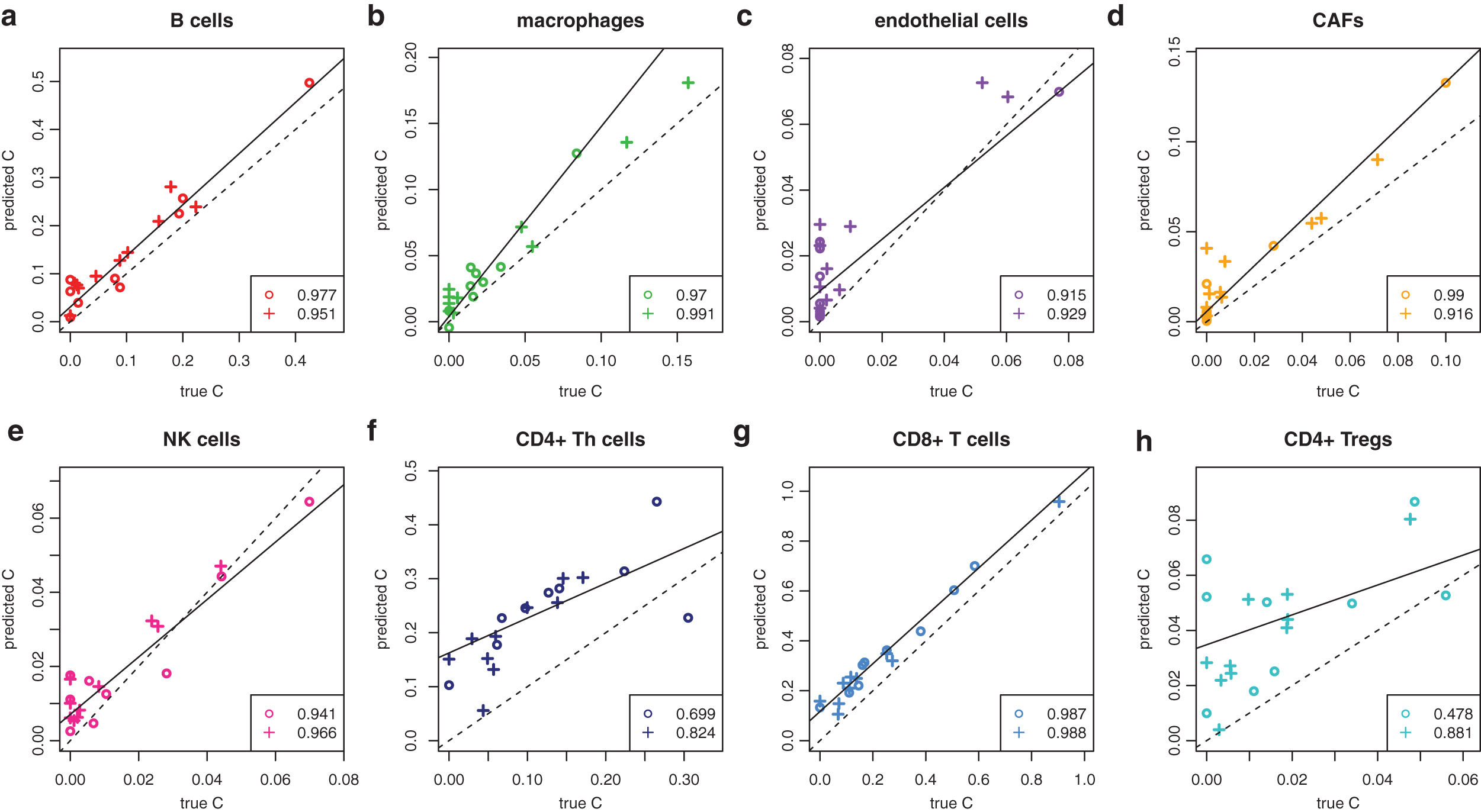
3.7. Loss-function learning shows similar performance as CIBERSORT for the dominating cell populations and improves accuracy for small populations and in the distinction of closely related cell types
Next we compared our model trained in section 3.6 with a competing method. For this, we generated 1000 test mixtures from our validation melanomas. We chose CIBERSORT (Newman et al., 2015) for comparison, because it was consistently among the best DTD algorithms in a broad comparison of five different algorithms on several benchmark data sets (Newman et al., 2015). We ran CIBERSORT on the test mixtures, using two distinct approaches: first, we uploaded our validation data to CIBERSORT using their reference profiles. The performance is summarized in Figure 6 as CIBERSORT
a
. We observed that the large population of B cells was estimated accurately, whereas smaller populations were inaccurate (NK cells, Tregs). Next, we uploaded our reference profiles and used the CIBERSORT gene selection (CIBERSORT
b
green) were predicted with high accuracy. However, the distinction of similar cell types such as CD4+ T helper cells and Tregs was compromised,
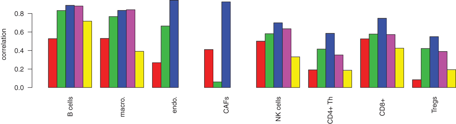
Performance comparison. The methods are from left to right: standard DTD with
Next, we tested whether our method would have also worked for bulk profiles generated by a different technology than the reference profiles. We used the scRNAseq-derived loss-function and the bulk profiles already described but replaced the reference profiles in X by microarray data downloaded from the CIBERSORT webpage. We rescaled the microarray matrix X such that the gene-wise means were identical to the scRNAseq data. Results are shown in Figure 6 in pink. Although accuracy was slightly reduced, we still improved on the CIBERSORT results.
3.8. Loss-function learning improves the decomposition of bulk melanoma profiles
All mixtures discussed so far were artificial because only 100 single-cell profiles were chosen randomly. They might differ significantly from mixtures in real tissue. Therefore, we generated 19 full bulk melanoma profiles by summing up the respective single-cell profiles. These should reflect bulk melanomas (Marinov et al., 2014). Our predictions are contrasted with the true proportions in Figure 7. Only the predictions for Tregs were compromised with
Deconvolution of melanoma tissues. The circles indicate melanomas from the validation data and plusses indicate those from the training data.
4. Discussion
We suggest using training data for loss-function learning for DTD to adapt the deconvolution algorithm to the requirements of specific application domains. The concept is similar to an embedded feature-selection approach in regression or classification problems. In both contexts, feature selection is directly linked to a prediction algorithm and not treated as an independent preprocessing step.
The main limitation of our method is the availability of training data. Other methods do not use, and cannot use, training data. In fact, the strength of loss-function learning results primarily from the additional information in training data with known cellular compositions. Such data are not always available, but with current improvements in FACS and single-cell sequencing technology, it is becoming increasingly available.
We described and tested a specific instance of loss-function learning using squared residuals for
The outer loss function L evaluates the fit of estimated and true cellular proportions in the training samples. We chose the correlation of estimated versus true quantities across samples, and no absolute measure of deviation such as
In summary, we introduced loss-function learning as a new machine-learning approach to the DTD problem. It allows us to adapt to application-specific requirements such as focusing on small cell populations or delineating similar cell types. In simulations and in an application to melanoma tissues, the use of training data allowed our method to quantify large cell fractions as accurately as existing methods and significantly improved the detection of small cell populations and the distinction of similar cell types.
5. Appendix
5.1. The choice of the objective function
The loss function (3) is not unique. However, Pearson correlation has advantages with respect to data normalization as shown in the following. First, note that
where aj is an arbitrary positive constant. This symmetry is important, since bulk and reference profiles must be normalized to a common mean across genes or to a common library size. A normalized reference profile
yields estimates
Note that
Here, we assume
The choice of the correlation in the definition of
Thus, the estimated cell frequencies are
In summary, data normalization makes tissue deconvolution a nonstandard deconvolution problem. The choice of correlation as loss function allows us to estimate cell frequencies independent of normalization factors.
5.2. Calculation of the loss-function gradient
The gradient
and
Then, we get
Thus, the gradient is given by the diagonal elements of
Footnotes
Author Disclosure Statement
The authors declare they have no conflicting financial interests.
Funding Information
This study was supported by BMBF (eMed Grant No. 031A428A) and DFG (FOR-2127 and SFB/TRR-55).