A Nested 2-Level Cross-Validation Ensemble Learning Pipeline Suggests a Negative Pressure Against Crosstalk snoRNA-mRNA Interactions in Saccharomyces cerevisiae

Abstract

The growing number of RNA-mediated regulation mechanisms identified in the past decades suggests a widespread impact of RNA-RNA interactions. The efficiency of the regulation relies on highly specific and coordinated interactions while simultaneously repressing the formation of opportunistic complexes. However, the analysis of RNA interactomes is highly challenging because of the large number of potential partners, discrepancy of the size of RNA families, and the inherent noise in interaction predictions. We designed a recursive two-step cross-validation pipeline to capture the specificity of noncoding RNA (ncRNA) messenger RNA (mRNA) interactomes. Our method has been designed to detect significant loss or gain of specificity between ncRNA-mRNA interaction profiles. Applied to small nucleolar RNA-mRNA in Saccharomyces cerevisiae, our results suggest the existence of a repression of ncRNA affinities with mRNAs and thus the existence of an evolutionary pressure leveling down such interactions.

1. Introduction

Evidence of the breadth of the role of ribonucleic acids in gene regulation are now multiplying. For instance, in eukaryotes microRNAs bind messenger RNAs (mRNAs) to control gene expression (He and Hannon, 2004), and in prokaryotes the OxyS RNA interacts with the fhlA mRNA to prevent ribosome binding and thus inhibit translation (Altuvia et al., 1998).

Among all noncoding RNAs (ncRNAs) already identified, the category of small nucleolar RNAs (snoRNAs) is of particular interest. snoRNAs form a large class of well-conserved small ncRNAs that are primarily associated with chemical modifications in ribosomal RNAs (rRNAs) (Scott and Ono, 2011). Recent studies revealed that orphan snoRNAs can also target mRNAs in humans (Sharma et al., 2016) and mice (Nguyen et al., 2016), and probably contribute to regulate expression levels. However, despite recent investigations there is no evidence to date that similar snoRNA-mRNA interactions occur in simpler unicellular microorganisms (Aw et al., 2016; Panni et al., 2017).

Of interest, it turns out that RNA-based gene regulation mechanisms have been primarily linked to higher eukaryotes (Mattick, 2004), although it is still not clear if this observation results from an incomplete view of RNA functional landscape or the existence of a negative pressure preventing RNA to interfere with other transcripts.

Our understanding of RNA-mediated regulation mechanisms significantly improved in recent years. In addition to well-documented molecular pathways (Altuvia et al., 1998), regulation can also occur at a higher level through global affinities between ncRNA and mRNA populations (Weill et al., 2015). Furthermore, Umu et al. (2016) showed another intriguing, yet complementary, level of control of gene expression that could explain discrepancies previously observed between expressions of mRNAs and the corresponding protein expressions in bacteria (Waters and Storz, 2009; Storz et al., 2011). In their study, the researchers extracted a signal suggesting a negative evolutionary pressure against random interactions between ncRNAs and mRNAs that could reduce translation efficiency. However, these results cannot be trivially extended to eukaryotes where the role of the nucleus has to be considered.

In this study, we investigated this phenomenon of avoidance of random interactions between ncRNA and mRNA in Saccharomyces cerevisiae. In particular, we focus our analysis on the bipartite interactome between snoRNAs and mRNAs. Indeed, the snoRNA family is an ancient and large class of ncRNAs for which the mechanism of mRNA avoidance could explain the small number of known interactions between snoRNAs and mRNAs in unicellular eukaryotes.

A major challenge of this analysis stems from the limited number of available curated snoRNAs sequences. Although we retrieved >6000 annotated mRNAs, we could only recover <100 snoRNAs (Sherman et al., 2004). Such disparity is a serious source of bias that should be carefully addressed. Therefore, we developed a customized ensemble learning pipeline to quantify the specificity of RNA binding profile between unbalanced RNA families.

First, we use state-of-the-art prediction tools to compute the snoRNA-mRNA interactome as the set of all interactions between snoRNAs and mRNAs. Then, we designed an ensemble learning pipeline to identify statistically significant biases in the distribution of binding affinities between classes of RNAs. Of importance, to remove any possible source of bias during the parametrization of classifiers, we introduce a second level of leave-one-out cross-validation (LOOCV) to avoid overfitting. Our results reveal that although different classes of snoRNAs exhibit distinct interaction patterns with mRNAs, this selective pressure is not as strong as initially anticipated. It corroborates previous hypothesis on prokaryotes, and suggests the presence of a phenomenon of avoidance of random interactions between ncRNAs and mRNAs in yeast.

2. Approach

We aimed to characterize the strength and specificity¹ of random ncRNA-mRNA interactions in S. cerevisiae, although our work primarily focuses on snoRNA-mRNA interactions. We relied on machine learning to estimate this specificity, as it is the key aspect classifiers rely on to make their prediction. Our dataset includes smaller categories of ncRNAs (e.g., spliceosomal RNAs) used for an additional control of our results.

We computed ncRNA-mRNA interactomes from ncRNAs and mRNAs sequences using two different state-of-the-art computational prediction tools [RNAup (Mückstein et al., 2006) and intaRNA (Wright et al., 2014)]. Those predictions are to serve as an approximation for the propensity of those ncRNAs to form crosstalk interactions with mRNAs. By using an ensemble learning pipeline, we approximated the specificities of interaction profiles in those interactomes. We also approximated the specificities of ncRNAs sequences with machine learning upon the Kmer compositions of the said sequences. The comparison of the approximated specificities highlights a global pressure inhibiting the affinity ncRNA-mRNA interactions in S. cerevisiae.

We finally completed this work by a collection of complementary control tests providing a better understanding of the limitations of this work. Data, code, raw results, and high resolution displays are available on an online repository (see the first reference: Soulé et al., 2020).

3. Methods

3.1. Dataset

3.1.1. Saccharomyces cerevisiae

We focus our study on a single organism: S. cerevisiae. Working on a single organism ensures that all the molecules coevolved and that their interactions were under the same evolutionary pressure. We also focus our study on a eukaryote to investigate the influence of the nucleus. Indeed, the nuclear membrane creates a confined environment that segregates molecules. Moreover, eukaryotes usually display more complex mechanisms and have more coding sequences than prokaryotes and archaea. Extending the study to several organisms, like Umu et al. (2016) did for instance, has been considered (in our case, the Saccharomyces genus). However, less data are available for other related yeasts and including more species increases the number of parameters to consider. We concluded that a multispecies study, although being interesting, was unrealistic yet. Finally, we excluded multicellular organisms to avoid problematic phenomena like specialized tissues.

For all those reasons, this study required a unicellular eukaryote offering a satisfactory number of identified RNA sequences and S. cerevisiae appeared to be the most suited model by being a model eukaryote organism with the greatest number of annotated sequences among unicellular eukaryotes.

All sequences were obtained from the manually curated Genolevure (Sherman et al., 2004) database.

3.1.2. ncRNA-mRNA interactome

The main input for this study is the ncRNA-mRNA interactome that is, all the ncRNA-mRNA interactions. Noticeably, we are referring to ncRNA-mRNA interactions as computational predictions instead of experimentally observed interactions. The probability of such event is conventionally approximated by the energy barrier and difference of entropy (Δg) between the structures of the two molecules and the structure of a potential complex (Mückstein et al., 2006). We work under the usual and reasonable assumption that, for two complexes i and j, if Δg_i < Δg_j then the complex i is more stable than the complex j and thus is more likely to form and be observed. To study the set of all potential ncRNA-mRNA complexes, we computed for all {ncRNA, mRNA} pairs the corresponding Δg using prediction tools (Section 3.2.1), thus resulting in two predicted ncRNA-mRNA interactomes: one for each prediction tool we used (Section 3.2.1).

We focused our study on the ncRNA-mRNA interactome for two reasons. First, the role of mRNA as temporary medium of genetic material makes it a central element in most cellular pathways. mRNAs are centerpieces of several mechanisms such as regulation (Waters and Storz, 2009; Storz et al., 2011; Umu et al., 2016) and splicing that might be impacted by crosstalk interactions. Second, ncRNAs (i.e., noncoding RNAs, which refers here to RNAs which are neither mRNAs, transfer RNAs, or rRNAs and also excludes miRNAs and siRNAs; Section 3.1.3) offer properties of interest for this study.

Indeed, the selected ncRNAs can be clustered into categories sharing similar properties, such as structure and length, which makes any comparison more meaningful. Those ncRNAs are also free from cellular mechanisms such as maturation or directed export that might generate noise. Finally, there is no observed interaction between those ncRNAs and mRNAs. As a consequence we can assume that the interactions we predict are opportunistic and not part of a defined biological pathway. A detailed description of ncRNAs labels is provided in Section 3.1.3.

We also considered two other practical aspects in this decision: maximizing the number of available annotated sequences and maximizing the number of crosstalk interactions (i.e., minimizing the number of known interactions). The first aspect directly impacts the statistical validity of any potential results, whereas the second is justified by the goal of this study, and the ncRNA-mRNA interactome satisfies both. To our knowledge, the largest set of ncRNA-mRNA interactions was published by Dudnakova et al. (2018). It comprises 448 snoRNC-mRNA interactions that amount to <0.1% of the interactome considered in this study.

Note: The study of Dudnakova et al. (2018) was published a few months after the first publication of this article. As we just mentioned, their results do not impact the validity of this study. However, they might offer the opportunity for complementary experiments, in particular to estimate the validity of the predicted interactions. Unfortunately, differences in the methods and datasets used make such experiments complex to perform. Those experiments will rather be part of a future work, based on this one, which will also benefit from newly found sequences.

3.1.3. ncRNA (noncoding RNA) labels

To conduct this study, we had to choose which of the mRNAs or ncRNA to label. The absence of structural properties in mRNA naturally inclined us to label ncRNA instead. We produced a five-label classification (Table 1) according to the gene ontologies based on both functional and structural properties. Of those five labels, two labels happen to be much more similar in terms of lengths and numbers. As a consequence, we performed all our tests with both the five labels dataset and a dataset limited to those two similar labels and are providing displays for both.

Table 1.

Numbers for the Two Datasets

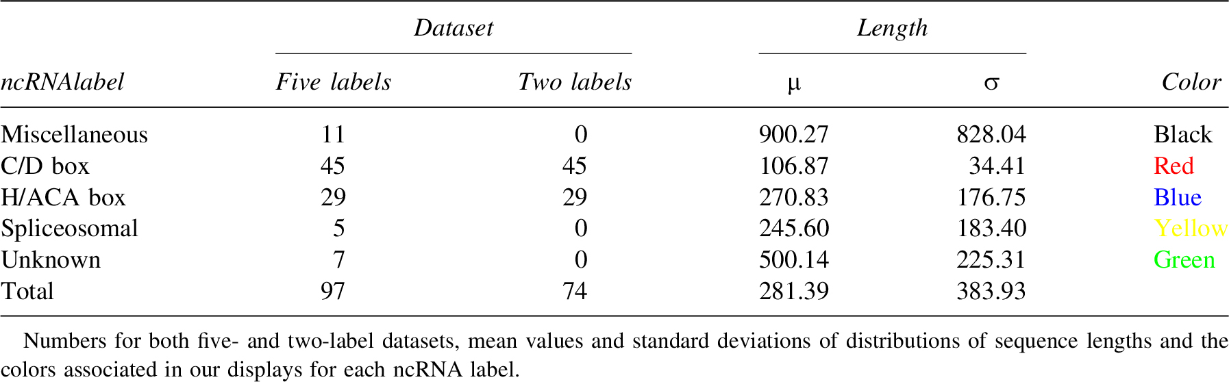
A complete description of all those ncRNAs is available elsewhere. For the sake of clarity, we will only provide a shorter description of each label in this article.

C/D box and H/ACA box ncRNAs are snoRNAs (small nucleolar RNA) involved in pre-rRNA maturation by performing two different modifications of specific bases. C/D box snRNAs are performing 2-O methylation, a methylation of the ribose. RNA has a short lifespan compared with DNA. By methylating the ribose, the rRNA is less vulnerable to degradation by bases or RNAses. In addition to this increased lifespan, this modification also impacts the rRNA structure by changing spatial constraints and decreasing the number of hydrogen bonds the modified base can form (Thuriaux et al., 2004, p. 200). H/ACA box snRNAs are performing pseudouridylation, an isomerization of uridines into pseudouridines. Pseudouridines have an extra NH group able to form supplementary hydrogen bonds. Those bonds stabilize rRNA structure (Thuriaux et al., 2004, p. 200).

Those two labels are the most consistent, both in numbers and internal similarities with both sequential constraints (boxes) and similar structures common to all the ncRNAs of a given label. Moreover, the lengths of ncRNAs are consistent inside each label and shorter than the ncRNA average (Fig. 4). Of importance, we will use these two groups (i.e., C/D box and H/ACA box ncRNAs) to study the existence of an evolutionary pressure on snoRNAs. The other groups described hereunder will be used as control and/or to suggest the generalization of the pressure to other classes of ncRNAs.

Spliceosomal ncRNAs share the common trait of being involved in the splicing process. However, all other properties vary.

Miscellaneous ncRNAs have been identified and their functions are known. However those functions are too specific and diverse to be gathered in any label but miscellaneous. Moreover, all other properties vary.

Unknown ncRNAs have been identified but, unlike miscellaneous ncRNAs, their functions remain unknown. Moreover, all other properties vary in an even wider range than the two previous labels.

3.2. Features description

This section describes the three metrics used in this study to produce the main sets of features: RNAup, IntaRNA, and Kmer composition similarity. Other basic features used as control, such as sequence length, are not described as they are straightforward.

3.2.1. RNA-RNA interactions prediction tools

To produce predicted interactomes, we use two different RNA-RNA interaction prediction tools: RNAup (Mückstein et al., 2006) and IntaRNA (Busch et al., 2008; Wright et al., 2014). As we are interested in nonspecific interactions, we preferred generalist prediction tools like those two overspecialized ones such as RNAsnoop (Tafer et al., 2010).

Both RNAup and IntaRNA implement the same core strategy. They compute the hybridization energies between the two RNAs and the accessibility (i.e., probability of being unpaired) for each interaction site. Those values are then combined to score potential interaction sites. The highest scoring sites are returned together with the free energy of binding. We can then retrieve the secondary structures of each individual RNA using constraint folding algorithms.

RNAup strictly implements this strategy thus predicting the optimal minimum free energy (MFE) compatible with the axioms. IntaRNA differs by two aspects. The first one is that the version of IntaRNA used in this study uses a slightly less recent version of Turner energies model. However, the differences between those versions are minor and are very unlikely to produce the observed dissimilarities. The second one is that IntaRNA adds a seeding step to reject interaction sites deemed unlikely. This extra step reduces the search space by focusing on the most promising ones and significantly reduces the runtimes compared with RNAup. An extensive description of the seeding procedure was presented by Bush et al. (2008). Comparative benchmarks place IntaRNA in the top of prediction tools with better scores than RNAup (Lai and Meyer, 2016; Umu and Gardner, 2017). Indeed, IntaRNA seems to predict interactions closer to the observed ones compared with predictions from other prediction tools, including RNAup. As a consequence, this heuristic seems well founded and efficient.

In this study we used this difference between RNAup and IntaRNA to predict two slightly different interaction modes. For each {ncRNA, mRNA} pair, we are assuming that RNAup outputs the optimal MFE regardless of its likelihood, whereas IntaRNA outputs a probably weaker but more realistic interaction. Because realistic interactions are more likely to be observed in the cell than the theoretical optima, any pressure should impact the first before the second. As a consequence, we aimed at highlighting such pressure by studying those two sets of interactions in parallel.

3.2.2. Kmer composition similarity

In addition to the two prediction tools mentioned in the previous subsection, we rely on a third source of input as a control: the similarity of the Kmer composition of ncRNA sequences. The term Kmer refers here to every possible sequence of nucleobasis of length K. This metric associates to each ncRNA the distribution of each Kmer in its sequence, including repetitions, represented as a vector (each dimension corresponding to a given Kmer). All vectors (one for each ncRNA) are gathered as a vector space suitable for machine learning (Section 3.3). We produced this third set of features to assess the specificity of the sequence and to provide a reference point to the two other sets of features.

All experiments involving Kmers have been made with K = 5 for two reasons. The first one is that 5 is the length of the average interacting zone in RNA-RNA interactions and so is a suitable length to capture any key subsequences impacting those interactions. The second one is that the number of Kmers to consider grows with the value of K. K = 5 offers the advantage of being both manageable in term of cost and also results in a number of dimensions comparable with the two other methods (i.e., RNAup and IntaRNA). We performed preliminary tests with others values, especially K = 6. Those tests showed little to no differences.

3.3. Ensemble learning pipeline

The overall goal of our machine learning approach (summarized in Fig. 1) was to investigate a possible bias affecting ncRNA-mRNA crosstalk interactions. To do so, we compare the specificity of ncRNA sequences with the specificity of ncRNA-mRNA interaction profiles. The specificity of ncRNA sequences is approximated by the ability of classifiers to predict the labels of ncRNAs from their Kmer composition. ncRNA-mRNA interaction profiles (which are, for each ncRNA, the predicted interaction scores against all mRNAs) are predicted using prediction tools and their specificity is approximated by the ability of classifiers to predict the labels of ncRNAs from those profiles.

FIG. 1.

Illustration of our ensemble learning pipeline. The process starts from RNAs data in orange. Each ncRNA will be associated to a vector in the vector spaces and will be attributed a label according to its ontology. From either ncRNAs sequences (Kmer) or both ncRNA and mRNAs sequences (IntaRNA, RNAup), a set of scores will be computed and used as features. Machine learning is finally used to produce the results we are presenting from those vector spaces. LOOCV, leave-one-out cross-validation; mRNA, messenger RNA; ncRNA, noncoding RNA; PCA, principal component analysis; RF, random forest.

Our utilization of machine learning in this project is challenging for two different reasons that justify all the following methodology choices: 1.

The ratios |vectors|/|features| of our datasets are problematic: 97 vectors for 6663 dimensions for the vector spaces built from the interactomes. Those ratios are the result of both cellular biology, because the number of mRNAs in a genome is always greater by several folds than the number of ncRNAs and the limited availability of annotated ncRNAs sequences, thus limiting as well the number of vectors. Those two issues are beyond our control and, to our knowledge, there is no way for us to significantly improve those ratios for S. cerevisiae without considerable drawbacks. Moreover, S. cerevisiae already has the greater number of annotated ncRNAs among similar organisms.

Our goal was neither to train a good classifier nor to classify unlabeled RNAs but to estimate how well the labels can be predicted from the different features. We are working under the reasonable assumption that a loss in performance between two sets of features implies that the lesser performing set is less specific (i.e., the features of a given ncRNAs class are less specific to this class). If the sets of features are related, like ours are, it would imply a leveling mechanism.

3.3.1. Leave-one-out cross-validation

Cross-validation refers in machine learning to partitioning the dataset into different sets to separate the data used to train the classifier and the ones used to test it. The goal of cross-validation is to ensure the credibility of the results produced.

We use a LOOCV technique for validation. For every vector v_i in our set V of vectors we train a classifier on the set (V − v_i) and test the resulting classifier on the vector v_i. The final accuracy is computed as the average of the accuracies for all vectors. This technique fits our dataset and its limited number of vectors. A more classical approach such as train validation test would have required us to use very small sets.

Of importance, also performed a second nested level of LOOCV to avoid any bias during the parametrization of the classifiers. This second level is described in Section 3.3.2 and illustrated in Algorithm 1.

Algorithm 1: 2-level_procedure (D f, $l n c$ )
Data: Given dataframe D (i.e., the vector space) and $l n c$ , the list of numbers of components to consider for the PCA
Result: Returns $d a c c u r a c y$ , dictionary of (vector, accuracy)
1 $d i c t d a c c u r a c y = \emptyset$ ;
2 for $v e c t o r v_{i} \in D$ do
3 $t e s t s e t = {v_{i}}$
4 $t r a i n s e t = D - {v_{i}}$
5 $b e s t n c = - 1$
6 $a c c u r a c y b e s t n c = - 1$
7 for $n c \in l n c$ do
8 $D' = D - {v_{i}}$
9 $D' = P C A (D', n c)$
10 for $v e c t o r v_{j} \in D'$ do
11 $s u b t e s t s e t = {v_{j}}$
12 $s u b t r a i n s e t = D' - {v_{j}}$
13 $c l a s s i f i e r = n e w R F c l a s s i f i e r ()$
14 $c l a s s i f i e r . t r a i n (s u b t r a i n s e t)$
15 $t m p a c c u r a c y =$
$c l a s s i f i e r . t e s t (s u b t e s t s e t)$
16 if $t m p a c c u r a c y > a c c u r a c y b e s t n c$
then
17 $b e s t n c = n c$
18 $a c c u r a c y b e s t n c =$
$t m p a c c u r a c y$
19 $D = P C A (D, b e s t n c)$
20 $c l a s s i f i e r = n e w R F c l a s s i f i e r ()$
21 $c l a s s i f i e r . t r a i n (t r a i n s e t)$
22 $d a c c u r a c y [v_{i}] = c l a s s i f i e r . t e s t (t e s t s e t)$
23 return $d a c c u r a c y$ ;

3.3.2. Principal component analysis

Because the ratio |vectors|/|features| is poor in the dataset, it may hinder the accuracy of the classifiers. Principal component analysis (PCA) is a standard method to improve this ratio by reducing the number of dimensions. The PCA uses an orthogonal transformation to build a set of uncorrelated features (components) from the initial features with the objective of maximizing variance (i.e., minimizing the information lost by transforming).

The number of components to transform is an important parameter that may influence the classifier accuracy. Performing preliminary tests to determine the best number would lead to a serious risk of overfitting. As a consequence we dynamically determined this number for each vector. The procedure is described in Algorithm 1. From the first LOOCV, the set of vectors V has been split into a set of pairs of a training set V′ = (V – {v_i}) and a test set {v_i}. For each pair, a second LOOCV is performed on V′ leading to another set of pairs of a training set V″ = (V′− {v_i}) = (V – {v_i, v_j}) and a test set {v_j}. Potential values for the number of components are tested and the one producing the best accuracy over V′ is selected and used on V to predict the label of v_i. As a consequence, the number of components to transform to is always selected independently from the test set.

Ideally, the set of potential values for the number of components would be 1,2,…,|V|. However the computation time grows linearly with the number of values tested. As a consequence we decided to use a subset of 1,2,…,|V| instead. Preliminary tests shows a light peak of performances at 8–10 components with a slight decrease before and after. As a consequence we tried all values from 1,2,…,20.

3.3.3. Random forest classifier

We chose to use ensemble learning and more specifically random forest (RF) classifiers over other methods and classifiers because of some anticipated properties of the datasets. Indeed, the limitations of prediction tools are likely to generate noise which RF are relatively resilient to Hastie et al. (2009, p. 596). Moreover, the interactions we aimed at capturing were likely to be complex and the size of the training set to be limited. Because RF can capture complex interactions and are simple to train (Hastie et al., 2009, p. 587) compared with other classifiers (Hastie et al., 2009, p. 587) they appeared to be a fitting candidate. Our implementation uses the python package Scikit-learn (Pedregosa et al., 2011).

As the name suggests, RF classifiers involve randomness. As a consequence, we repeated the procedure and display distributions to counterbalance the variation of the predictions. Preliminary results show that the average accuracies of those distributions converge (10⁻⁴) within the first 500 runs. However we decided to double this value to add a comfortable security margin.

3.3.4. Dummy classifier

A second classifier is trained in parallel to serve as a control. As the name “dummy” suggests, it is not an actual classifier but a heuristic randomly generating labels for the test set according to the probabilities distribution it extracted from the training set. As the dummy classifier is always trained and tested on the same sets as its RF counterparts, it appears to be a suitable solution to produce a sound control while using LOOCV and using unbalanced labels. However, as all dummy classifiers produced extremely close performances, we decided to display only one of the dummy classifiers in each display instead of one per other classifier for the sake of clarity. Please note that the dummy classifier is unaffected by PCA as it does not consider the features.

3.3.5. Performance metric for a multi-label dataset

The number of labels in our datasets prevents straightforward use of some classical displays such as ROC curves. A single prediction can indeed be, for instance and at the same time, both false positive for a given label and true negative for another. As a consequence we have TPR + FPR + TNR + FNR ≥ 1 ([true, false] [positive, negative] rate) and plotting one ROC curve for each label offers little readability. As a consequence we instead chose to use displays based on accuracy (Accuracy = Precision = |Correct Predictions|/|Predictions|)).

3.4. Main experiments

As described in Sections 3.2 and 3.1.3, our work associates each ncRNA with three vectors of features ({Kmer, intaRNA, and RNAup}) and a label. By doing so we produced three vector spaces that are suitable for machine learning. We consider that the ability of the classifiers to predict those labels from a given set of features reflects how specific those features are to those labels. Therefore, the goal of the machine learning procedure described in Section 3.3 is to assess the specificity of the sets of features regarding the labels.

Figure 2 displays the distribution of the accuracies of the classifiers for all three kinds of features with two or five labels. The combination of LOOCV (Section 3.3.1) and the inherent randomness of RF classifiers (Section 3.3.3) lead us to produce and display distributions of accuracies instead of a single value. Exact mean values (μ) and standard deviations (σ) values for all those distributions are given aside in Table 2. The best accuracies are obtained from the Kmer similarity scores with 86.3% of correct prediction with two labels and a standard variation of only 0.31%. Results obtained from scores predicted by RNAup are less accurate but are still very distinct from the control with no overlap. However, results obtained from scores predicted by IntaRNA are significantly less accurate to the point that the distribution overlaps with the control. Results obtained with five labels display a similar hierarchy between Kmer, RNAup, and IntaRNA with the addition of an expected global loss of accuracy. Indeed, the increased number of labels to predict makes the problem harder as shown in the important drop of accuracy of the control. However, Kmer, RNAup, and IntaRNA appear to be all the more resilient than the control to this change.

FIG. 2.

Distribution of accuracies of 1000 classifiers following specifications of Section 3.3. Each row corresponds to either a set of features ({Kmer, RNAup, intaRNA}; Section 3.2) or the control (Section 3.3.4) associated with a number of labels ({2, 5}; Section 3.1.3). Mean values and standard deviations for all distributions are given in Table 2.

Table 2.

Means and Standard Deviations

	Two labels		Five labels
	μ	σ	μ	σ
Control	0.517	0.057	0.316	0.044
Kmer	0.863	0.031	0.724	0.03
RNAup	0.794	0.032	0.699	0.03
IntaRNA	0.675	0.04	0.555	0.037

Mean values (μ) and standard deviations (σ) for all distributions displayed in Figure 2.

The difference of performances given in Figure 2 between the classifiers working on Kmer compositions and the ones working on either set interaction profiles implies (according to the assumptions we made) that the interaction profiles predicted by either tool are less specific than the ncRNAs sequences, despite the predictions being based on those very sequences. This suggests the existence of a leveling mechanism, possibly an evolutionary pressure against very specific snoRNA-mRNA interactions patterns (which is not the same as an evolutionary pressure against snoRNA-mRNA interactions in general).

Moreover, the gap between the two prediction tools implies that interaction profiles predicted by IntaRNA are significantly less specific than the ones predicted by RNAup. The interaction profiles predicted by RNAup also seem to be the closest to the ones produced from Kmer similarity scores and thus seem to give the most accurate account of the specificities of the sequences. This observation, together with the previous one and the difference between the two prediction tools described in Section 3.2.1, suggests that probable interactions (i.e., the ones predicted by IntaRNA) are more inhibited than the potential optimal ones (i.e., the ones predicted by RNAup). This first observation is coherent with the influence of an evolutionary pressure as the inhibition of probable interactions would have a greater impact than the inhibition of potential optimal ones that are less likely to form.

Figure 3 is a different presentation of the results given in Figure 2. Raw results from the classifiers are unitary predictions (i.e., predictions of the label of one vector). We gathered those unitary predictions for each vector, thus producing an averaged accuracy for each of them. Figure 3 aims at highlighting variations inside the distribution given in Figure 2. Please note that each column corresponds now to a different set of features while the upper row provides the results with two labels and the lower row provides the results with five labels. Each line corresponds to ncRNA, the length reflecting the accuracy of predictions made for this ncRNA label, whereas the color corresponds to its label. Please also note that lines are sorted by accuracies. As a consequence, the order varies in all those six subgraphs.

FIG. 3.

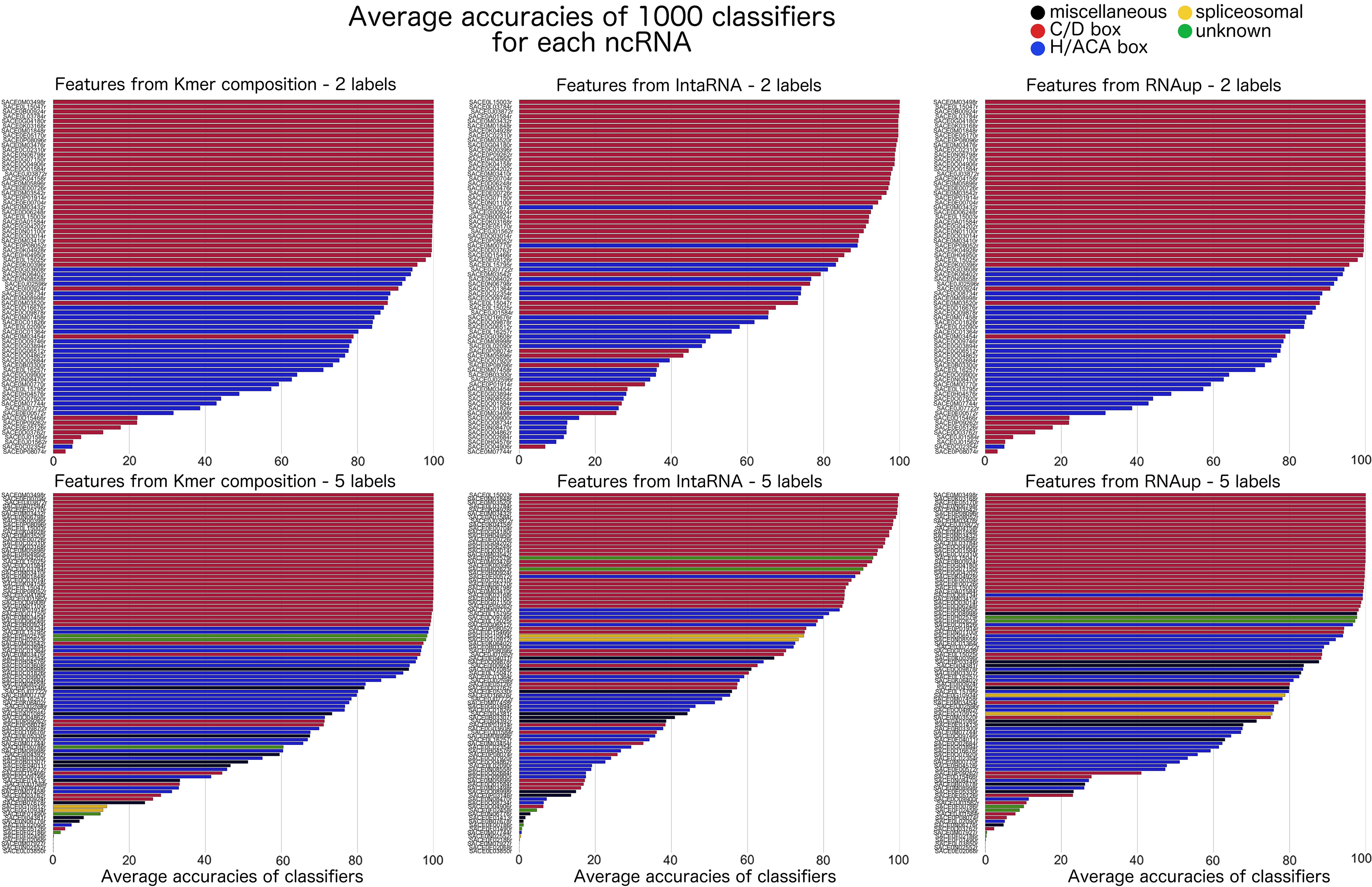
Average accuracies of classifiers for each vector (i.e., ncRNA) over 1000 tests. Each column corresponds to a set of features ({Kmer, RNAup, intaRNA}; Section 3.2). The first row displays the results with five labels and the second with two labels (Section 3.1.3). Each colored line in those six displays corresponds to a (vector/ncRNA). The length of the line represents the averaged accuracy of the 1000 classifiers for the corresponding (vector/ncRNA). The color of the line corresponds to the label of the associated (vector/ncRNA). Please note that (vectors/ncRNAs) are sorted according to the accuracy associated to them. As a consequence the order is different in all six graphs.

The drop of accuracy observed in Figure 2 between Kmer similarity scores, RNAup predicted scores, and IntaRNA scores is also given in Figure 3 as a more concave slope for better performing sets of features. However, Figure 3 also provides variations of accuracies from one label to the other. C/D box RNAs (red) are the most noticeable group as those RNAs are, on average, extremely well predicted with all features and either two and five labels. H/ACA box RNAs (blue), on the contrary, seem to be harder to predict from Kmer similarity scores or RNAup predicted scores than C/D box RNAs but show a dramatic drop of accuracy in predictions made from IntaRNA predicted scores. Prediction accuracies of the three remaining labels vary from a set of features to the other and even inside a label for a given set of features. We have been unable so far to determine if this was only because of a lesser number of vectors for those labels or because of other parameters.

Results given in Figure 3 complement our previous observations as the {Kmer, RNAup, IntaRNA} hierarchy is still clearly observable. However, Figure 3 provides a phenomenon invisible in Figure 2: the variance in predictions accuracy between the label, especially regarding C/D box RNAs and H/ACA box RNAs. Indeed, predictions for C/D box RNAs (red) are always the most accurate, whereas predictions for H/ACA box RNAs (blue) clearly fall behind. This variance goes from a limited difference (most predictions for H/ACA box RNAs are still >80% accuracy in predictions from Kmer similarity scores with two labels, cf. top left graph) to a dramatic drop (predictions from IntaRNA predicted scores with two labels, cf. top right graph). Prediction accuracies of the three remaining labels vary from a set of features to the other and even inside a label for a given set of features. We have been unable so far to determine if this was only because of a lesser number of vectors for those labels or because of other parameters. However, the predictions of the three remaining labels display accuracies similar to the ones of predictions for H/ACA box RNAs. Because the dataset contains more H/ACA box RNAs than the three other labels put together, this similarity stresses that H/ACA box RNAs are way harder to predict than C/D box RNAs. Further discussions of this difference of performances between labels require to first introduce Figure 4.

FIG. 4.

Normalized distributions of scores predicted by IntaRNA (left), scores predicted by RNAup (middle) and lengths of sequences (right) for each ncRNA label. Scores are in kcal/mol. Please note that scores from both IntaRNA and RNAup approximate a difference of entropy (Δg) and are therefore negative. A lower score thus suggests that the interaction is stronger.

To investigate the drop in accuracy between predictions made from scores predicted by RNAup and IntaRNA, we plotted distributions of scores as box plots for each tool (left and middle) and for each ncRNA labels (colors). We also plotted the distributions of the lengths of ncRNAs sequences (right, please note that the influence of length results is discussed in Section 3.5.2). The results are given in Figure 4. The color code is the same as in Figures 2 and 3. Figure 4 shows that RNAup is not only outputting stronger scores (entropy scores are negative; Section 3.1.2) but also preserves distinctions between the labels, especially between C/D box RNAs and H/ACA RNAs scores. This observation is coherent with the better performances of classifiers learning from the interactome predicted with RNAup. However, the important drop in accuracies given in Figure 3 on scores predicted with IntaRNA with two labels shows that RF classifiers are able to capture variations (Figs. 2 and 3) that the extremely similar distributions of those two labels in Figure 4 fail to display. This observation suggests that the global inhibition that is shown by the drop in the averages of both RNAup and IntaRNA scores is also a leveling phenomenon rather than a “linear” inhibition.

3.5. Additional experiments

3.5.1. Impact of boxes on predictions

Among the five labels we are considering, two correspond to ncRNA classes defined by the presence of “boxes” in the sequence: C/D box snoRNAs and H/ACA box snoRNA. Those boxes are small and their consensus sequences are flexible (C: RUGAUGA, D: CUGA, H: ANANNA, ACA: ACA) yet they might bias our results. Indeed, if a few Kmers were to accurately capture those boxes, a classifier might output accurate prediction by only considering those Kmers.

To investigate this matter, we performed a brute force feature selection algorithm specific to RF classifiers: the Boruta algorithm. This algorithm tests each feature, estimates its contribution to the classification and produces the list of features considered to be crucial for a given threshold of confidence (i.e., p-value, default = 0.05). Results show that only 50% or less of the critical features are compatible with a consensus sequence, even in the two-label dataset (restrained to C/D box and H/ACA boxes snoRNAs only). Even if this measure is only an upper bound of the influence of those boxes since the compatible Kmers may be capturing parts of the sequence that are not actually boxes, it shows that the majority of critical features are not related to boxes. As a consequence, we can exclude the possibility that the predictions given in Figures 2 and 3 are based on a limited number of Kmers capturing the boxes.

3.5.2. Impact of sequence lengths on RNA-RNA interaction predictions

The third panel of Figure 4 provides the distributions of lengths of ncRNAs for all labels, each label being represented by a boxplot in its usual color. Length distributions vary from a label to another with two visible groups of labels: C/D box, H/ACA box, and spliceosomal labels (resp. red, blue, and yellow) distributions have the lowest deviation, whereas miscellaneous and unknown labels (respectively, black and green) present a wider distribution with overall longer sequences. The challenge posed by lengths of mRNAs targets has been explored by Lai and Meyer (2016) and Umu and Gardner (2017). Their results show that the accuracy of prediction tools typically drops as the length of the target increases above 300 nb. However, among the prediction tools tested, IntaRNA seems relatively resilient to an increase of the length of the target. On the contrary RNAup performances are significantly reduced. Cutting down the targets into subsequences of manageable length is not suited for this study as we need one score per {ncRNA, mRNA} pair. Moreover, we would like to propose to interpret this drop not only as a flaw of RNAup but as an illustration of the difference we described in Section 3.2.1. Yet the predictions scores for miscellaneous and unknown labels (respectively, black and green) are to be treated with caution.

A second problem to consider is that the features we used are not independent of sequence lengths. Indeed, a longer sequence will contain more Kmers and Figure 4 suggests a partial correlation between scores and length. To investigate this issue we repeated the ensemble learning procedure with the length as the only feature. Results show that predictions using length are accurate (μ = 0.856 and σ = 0.012 with the two-label dataset, μ = 0.651 and σ = 0.013 with the five-label dataset) but are slightly outperformed by the ones trained on RNAup scores over the five-label dataset and over both datasets by the ones trained on Kmer composition. Those results suggest that sequence lengths are specific to each label but are not the only variation captured by the classifiers.

3.5.3. Overlapping of predicted interaction zones with observed interaction zones

Another potential bias to investigate was the possibility that interaction profiles of a ncRNA class might be similar because of a part of the sequence common to all ncRNAs of the class being overrepresented in predicted interactions. To investigate this potential bias, we scanned the sequences of C/D box snoRNAs in the dataset looking for the consensus sequences. We excluded C/D box snoRNAs with ambiguous sites (i.e., more than one match with the consensus sequences of either box in the parts of the sequences those boxes are supposed to be). We then looked for any intersection between the area interacting with rRNAs in observations (i.e., 3rd to 11th nucleotides upstream from D box) and the interaction zones predicted by RNAup. Among the interaction zones involving the 35 selected C/D box snoRNAs candidates, none overlapped with the observed interaction zones. We did not perform the same test on H/ACA box snoRNAs because the lesser specificity of the consensus sequences makes the localization of the zones problematic. However, the results on C/D box snoRNAs strongly suggests that there is no such bias in the interaction profiles.

4. Conclusion

Our results enabled us to identify the signature of an evolutionary pressure against random interactions between ncRNAs and mRNAs in S. cerevisiae. Presumably, as previously observed in prokaryotes and archaea, this phenomenon aims at increasing the translation efficiency (Umu et al., 2016). In addition, it may also prevent ncRNAs from being diverted from their role.

Although our dataset includes various types of ncRNAs, the vast majority of them are snoRNAs. Our conclusions are therefore primarily applicable to snoRNAs, even if our data do not exclude that it could be generalized to other ncRNAs. Of interest, the (old) age of the snoRNA family suggests that it could be the trace of a fundamental biological process used by primitive microorganisms. The absence (to our knowledge) of experimental evidences of snoRNA-mRNA interactions in unicellular eukaryotes tends to support our conclusions. By contrast, the existence of known interactions between orphan snoRNAs and mRNAs in human or mice (Nguyen et al., 2016; Sharma et al., 2016) opens a legitimate debate about the necessity and specificity of such mechanisms in animals.

Footnotes

Author Disclosure Statement

The authors declare they have no conflicting financial interests.

Funding Information

This study was supported by the McGill University, the École Polytechnique, the INRIA, the NSERC, and the FQRNT.

References

Soulé

, Steyaert

J.-M.

, and Waldispühl

2020. Repository for Code, Data and HR Figures, csb. cs.mcgill.ca/nested_loocv_pipeline. [Online].

Altuvia

, Zhang

, Argaman

, et al. 1998. The Escherichia coli OxyS regulatory RNA represses fhlA translation by blocking ribosome binding. EMBO J. 17, 6069–6075.

J.G.A.

, Shen

, Wilm

, et al. 2016. In vivo mapping of eukaryotic RNA interactomes reveals principles of higher-order organization and regulation. Mol. Cell. 62, 603–617.

Busch

, Richter

A.S.

, and Backofen

2008. IntaRNA: Efficient prediction of bacterial sRNA targets incorporating target site accessibility and seed regions. Bioinformatics, 24, 2849–2856.

Dudnakova

, Dunn-Davies

, Peters

, et al. 2018. Mapping targets for small nucleolar RNAs in yeast. Wellcome Open Res. 3, 120.

Hastie

, Tlbshirani

, and Friedman

2009. The elements of statistical learning: Data mining, inference, and prediction. Springer Science & Business Media.

, and Hannon

G.J.

2004. MicroRNAs: Small RNAs with a big role in gene regulation. Nat. Rev. Genet. 5, 522–531.

Lai

, and Meyer

I.M.

2016. A comprehensive comparison of general RNA-RNA interaction prediction methods. Nucleic Acids Res. 44, e61.

Mattick

J.S.

2004. RNA regulation: A new genetics?. Nat. Rev. Genet. 5, 316–323.

10.

Mückstein

, Tafer

, Hackermüller

, et al. 2006. Thermodynamics of RNA–RNA binding. Bioinformatics, 22, 1177–1182.

11.

Nguyen

T.C.

, Cao

, Yu

, et al. 2016. Mapping RNA-RNA interactome and RNA structure in vivo by MARIO. Nat. Commun. 7, 12023.

12.

Panni

, Prakash

, Bateman

, et al. 2017. The yeast noncoding RNA interaction network. RNA, 23, 1479–1492.

13.

Pedregosa

, Varoquaux

, Gramfort

, et al. 2011. Scikit-learn: Machine learning in python. J. Mach. Learn. Res. 12, 2825–2830.

14.

Scott

M.S.

, and Ono

2011. From snoRNA to miRNA: Dual function regulatory non-coding RNAs. Biochimie, 93, 1987–1992.

15.

Sharma

, Sterne-Weiler

, O'Hanlon

, et al. 2016. Global mapping of human RNA-RNA interactions. Mol. Cell. 62, 618–626.

16.

Sherman

, Durrens

, Beyne

, et al. 2004. Génolevures: Comparative genomics and molecular evolution of hemiascomycetous yeasts. Nucleic Acids Res. 32(Database issue), D315–D318.

17.

Storz

, Vogel

, and Wassarman

K.M.

2011. Regulation by small RNAs in bacteria: Expanding frontiers. Mol. Cell. 43, 880–891.

18.

Tafer

, Kehr

, Hertel

, et al. 2010. RNAsnoop: Efficient target prediction for H/ACA snoRNAs. Bioinformatics, 26, 610–616.

19.

Thuriaux

, Martin

, Blondel

, et al. 2004. Les Organismes Modèles: La Levure. Belin.

20.

Umu

S.U.

, and Gardner

P.P.

2017. A comprehensive benchmark of RNA-RNA interaction prediction tools for all domains of life. Bioinformatics, 33, 988–996.

21.

Umu

S.U.

, Poole

A.M.

, Dobson

R.C.

, et al. 2016. Avoidance of stochastic RNA interactions can be harnessed to control protein expression levels in bacteria and archaea. Elife, 5. DOI: 10.7554/eLife.13479

22.

Waters

L.S.

, and Storz

2009. Regulatory RNAs in bacteria. Cell, 136, 615–628.

23.

Weill

, Lisi

, Scott

, et al. 2015. MiRBooking simulates the stoichiometric mode of action of microRNAs. Nucleic Acids Res. 43, 6730–6738.

24.

Wright

P.R.

, Georg

, Mann

, et al. 2014. CopraRNA and IntaRNA: Predicting small RNA targets, networks and interaction domains. NAR, 42(Web Server issue), W119–W123.