Human MicroRNA Target Prediction via Multi-Hypotheses Learning

Abstract

MicroRNAs are involved in many critical cellular activities through binding to their mRNA targets, for example, in cell proliferation, differentiation, death, growth control, and developmental timing. Prediction of microRNA targets can assist in efficient experimental investigations on the functional roles of these small noncoding RNAs. Their accurate prediction, however, remains a challenge due to the limited understanding of underlying processes in recognizing microRNA targets. In this article, we introduce an algorithm that aims at not only predicting microRNA targets accurately but also assisting in vivo experiments to understand the mechanisms of targeting. The algorithm learns a unique hypothesis for each possible mechanism of microRNA targeting. These hypotheses are utilized to build a superior target predictor and for biologically meaningful partitioning of the data set of microRNA–target duplexes. Experimentally verified features for recognizing targets that incorporated in the algorithm enable the establishment of hypotheses that can be correlated with target recognition mechanisms. Our results and analysis show that our algorithm outperforms state-of-the-art data-driven approaches such as deep learning models and machine learning algorithms and rule-based methods for instance miRanda and RNAhybrid. In addition, feature selection on the partitions, provided by our algorithm, confirms that the partitioning mechanism is closely related to biological mechanisms of microRNA targeting. The resulting data partitions can potentially be used for in vivo experiments to aid in the discovery of the targeting mechanisms.

1. Introduction

MicroRNAs are short RNA sequences of ∼22 nucleotides that inhibit or repress gene expression. They perform as a guide to bind the RNA-induced silencing complex to sequence-specific locations on mRNAs to silence them (Agarwal et al., 2015). These specific locations are called target sites, and discovering the functionality of each microRNA depends on recognition of its target sites. MicroRNAs can control many critical cell processes such as proliferation, differentiation, cell death, growth control, and developmental timing (Lin and Gregory, 2015). Dysfunction of microRNAs could lead to tumor development and cancer in organs such as the lung, brain, colon, and breast in addition to causing hematopoietic cancers (Jansson and Lund, 2012).

Despite the importance of microRNAs, the detailed mechanism of microRNA target binding is poorly known. Laboratory experiments for finding targets are very slow and costly; therefore, there is a huge demand for computational approaches. In the last decade, dozens of algorithms, with a variety of approaches and techniques, have been developed. These methods are either specific for a few species or general for any kind. Methods for vertebrates include TargetScan and TargetScanS (Lewis et al., 2003, 2005), miRanda (Enright et al., 2004; John et al., 2004), DIANA-microT (Kiriakidou et al., 2004), and for flies RNAhybrid (Rehmsmeier et al., 2004). Some general tools are miTarget (Kim et al., 2006) and MicroInspector (Rusinov et al., 2005).

The early computational approaches for target recognition were rule based, that is, they had a set of discriminative rules derived from experimental and biological knowledge, such as minimum free energy (MFE), duplex binding pattern, or target accessibility. Some popular rule-based tools are RNAhybrid, TargetScan, miRanda, and MirBooking (Weill et al., 2015). MirBooking is one of the recent rule-based methods that simulate the microRNA and mRNA hybridization competition and cellular conditions to improve the accuracy of target prediction. In the last several years, with the increase of relevant data sets, data-driven methods have been attempted. These methods use sophisticated machine learning (ML) and statistical models to learn more discriminative features for target identification (Yue et al., 2009). Some popular data-driven tools are TargetSpy (Sturm et al., 2010), miRanda-mirSVR (Betel et al., 2010), and Avishkar (Ghoshal et al., 2015). However, such methods have yet to resolve the issue of high false-positive rate. The innovation of more advanced sequencing techniques, and therefore more precise data sets, along with recent advances in ML methods, could lead to the development of more accurate algorithms.

The microRNA targeting process has not been well understood; biologists are especially interested in approaches that may provide insights about the mechanisms of target recognition. Recent experimental studies of microRNA targeting reveal that there are multiple and different mechanisms for this process, whereas the earlier belief was merely based on seed match of microRNA and target site sequences (Cloonan, 2015). Currently, it is still not clear how many different and exclusive mechanisms guide microRNA targeting; therefore, computational models, which not only work well but also give insight into the biological mechanisms, are very desirable. Some ML techniques such as Bagging and Boosting or Random Forest aim to learn multiple hypotheses from the input data, but they do not provide any clue to check if these hypotheses are biologically meaningful or not. Biologically meaningful features here mean those characteristics that have been experimentally confirmed to be part of a microRNA targeting mechanism, such as appearance of adenine at the far 3′ end of a target site.

In this article, we introduce a multi-hypotheses learning (MHL) algorithm (Mohebbi et al., 2019) that aims at not only improving the performance of classifiers on microRNA targeting data but also meaningfully partitioning the data set per these learned hypotheses. MHL uses these hypotheses to predict microRNA targets with a superior performance. Moreover, the biologically meaningful partitions created by MHL could be used for further understanding the targeting mechanisms or to discover new target determinants. To verify our approach, we evaluated our method on human and mouse data. The results show that the partitioning is indeed biologically meaningful. Moreover, significant performance improvements on target prediction confirm learning multiple hypotheses can help outperform top ML algorithms such as RandomForest and deep learning (DL) models. Feature analysis of the partitions produced by MHL reveals interactions in microRNA and target duplex that are verified by the biology literature. This supports our conjecture that MHL could aid to mine meaningful features, which could be used as part of in vivo experiments.

2. Data Sets

The success of data-driven methods critically relies on the quality of the data. To build the most accurate models and the most realistic evaluations, we extracted our data from mirTarBase (Hsu et al., 2014), one of the most up-to-date data sets and the most referenced resource for microRNA target prediction research. In particular, mirTarBase contains more than 360,000 experimentally validated microRNA–target duplexes from 18 different species. This data set is publicly available and is subject to IRB Waiver. We are mostly interested in testing our ML method with both human and mouse records.

From mirTarBase, human and mouse microRNA–target duplexes were extracted whose secondary structures have been provided in research articles. Such duplexes were selected as positive samples for our method. However, negative samples are not directly available. Theoretically, any stretch of an appropriate length other than the real target in the 3′-UTR of a targeted mRNA gene can be considered a negative target of the corresponding microRNA. We randomly selected 10 locations in the 3′-UTR of a targeted mRNA gene to pick up the negative samples for each positive sample with a ratio of 10:1. Each sample is a pair of microRNA sequence of length 22 and a site sequence of length 25, which is real target site for positive samples or a negative site that is not a target for the microRNA.

2.1. Test set and training set

We have one training set and two test sets. The human data set is split 80% to 20% into the training set and human test set. All mouse data compose our second test set. In the human data extracted from mirTarBase, there are 322 unique microRNAs, 3651 target site sequences, and 3722 pairs of microRNA and target sites. On average, each microRNA has >10 targets sites. If we randomly select test set samples from the whole database, the odds of having many microRNAs in both test and training sets is high. To avoid such overlaps and to have the most reliable test set, we indexed pairs of microRNA and target sites by microRNA sequence. In addition, to make a test set with a similar distribution to that of the whole data set, we sort samples by microRNA sequences, put four consecutive (based on the sorting order) microRNA sequences and all their target and nontarget sites in the training set, then one microRNA sequence and all its targets and nontargets into the human test set, and so on. In this way and in terms of microRNA sequence, not only do the human test set and training set have no overlaps but also the test set has very similar distribution to that of the whole database. Both test sets and training sets have ratio of 1:10 for positive versus negative. The human test set consists of 6127 samples (557 positives vs. 5570 negatives), and the total size of the mouse test set is 517.

3. Materials and Methods

In this section, we introduce a feature selection approach that is biologically meaningful and is more efficient for microRNA targeting than common data mining feature selection methods. Data mining algorithms may not be applied directly to this problem because each sample is composed of sequences of microRNA and target, and the microRNA sequence is identical among its positive(s) and its negative samples. To verify this thought, we ran Weka (Witten et al., 2016), a data mining package, to extract the most significant features from samples of a microRNA sequence concatenated to a target sequence. All microRNA sequence nucleotides were excluded from selected features set and that is because the microRNA sequence is the common part of both positive and negative samples; therefore, feature selection algorithms consider the common part as a none determinant factor for classifying the samples. To cope with this problem, features must be defined based on correlations of microRNA and its target nucleotides rather than merely on sequences of nucleotides. In addition, and to incorporate biological knowledge of microRNA targeting, we extracted features from the secondary structure of a duplex associated with every sample.

We researched on the most recent discoveries on the mechanisms of microRNA targeting and customized RNAfold (Lorenz et al., 2011), a widely used secondary structure prediction tool for RNA sequences, to predict a specific structure for a pair of microRNA and target sequences that mimic the biological mechanisms of microRNA targeting. RNAfold is a general tool for secondary structure prediction, and it could predict structures in which microRNA or target site sequences bind to themselves or to each others in any ways. On the other side and biologically, sequences of microRNA and target sites should not make base pairs with themselves but with the other sequence. To guide RNAfold prediction for the purpose of microRNA targeting and include information about in vivo process of microRNA target binding, we tuned RNAfold to predict the structure of duplex based on rules we collected from biological literatures explaining the actual mechanisms of microRNA targeting.

The seed part of a microRNA consists of the nucleotides number 2 to 8 from the 5′ end of the microRNA (Lewis et al., 2003). It is believed that the process of nucleotide binding between the microRNA and its mRNA target starts from this region (Schirle et al., 2014). When the binding in the seed region is continuous for 6 to 8 bps, it is called a canonical seed; otherwise, it is called noncanonical (Loeb et al., 2012). Although the seed binding is considered the most important identifier for microRNA targets in mammals (Peterson et al., 2014), a recent study shows that it is not the only mechanism for microRNA targeting (Cloonan, 2015). To have a more comprehensive model, we considered correlations that occur not just in the seed region but also in all other regions across a microRNA and its target.

3.1. MicroRNA duplex secondary structure prediction

RNAfold predicts the most stable secondary structure of a single RNA sequence. To use it for predicting microRNA and target site duplexes, we concatenated microRNA and target site sequences with a subsequence of length 4 “X”s in between, as shown in Figure 1. This sequence of length 4 is the shortest sequence that we could add and still get the same MFE for the structure as the MFE we get from RNAcofold (Lorenz et al., 2011) when it predicts the duplex between microRNA and target site.

FIG. 1.

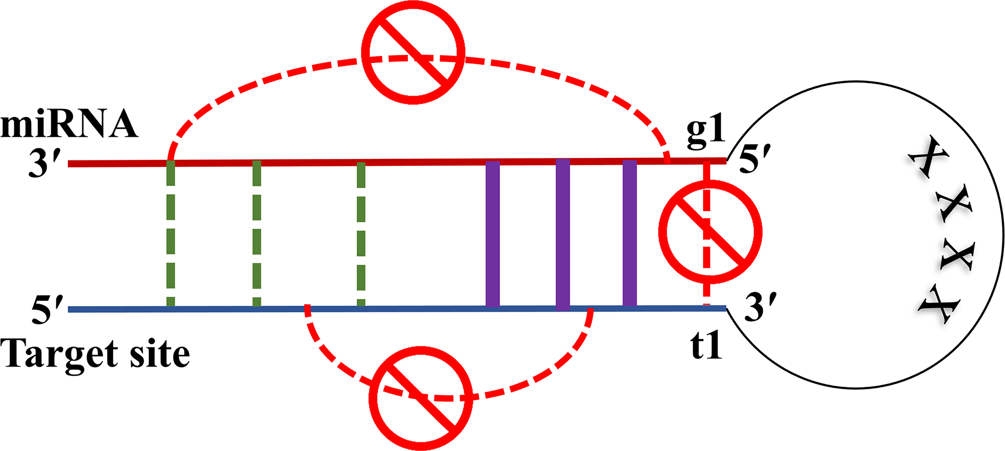
RNAfold customization for a microRNA (miRNA) –target duplex; sequences of microRNA and target site are concatenated with a subsequence of length 4 “X”s in between. Base pairing among nucleotides of one sequence is prohibited, either for microRNA or for the target site. A structural study on the mechanism of microRNA targeting (Schirle et al., 2014) reveals that the nucleotide in t1 goes into a pocket inside the Argonaute protein structure and does not pair with the corresponding nucleotide on microRNA. We added a constraint to prevent t1 from such a base pairing with the microRNA. Base pairs (purple color) are enforced through the customization if the corresponding nucleotides are complimentary matching. Black dashed lines show possible locations of valid base pairs, and we let RNAfold to predict them.

RNAfold can have a constraints file as an input parameter to enforce the structure prediction process to occur based on a user's domain knowledge. Here, we set these constraints for the microRNA targeting mechanism, to include rules for base pairs that are biologically expected to happen in seed, and rules prohibiting microRNA nucleotides from binding to microRNA itself. Similarly, there are rules avoiding target site sequence to bind over itself. We applied all these rules for duplexes with canonical seeds, while releasing seed base pairing constraints for noncanonical seeds.

Biological experiments and in vivo methods reveal several mechanisms for microRNA targeting (Cloonan, 2015). The earliest discovered and the most dominant method of targeting was based on seed matching (Lewis et al., 2005; Friedman et al., 2009). In this mechanism, microRNA carried by the Argonaute protein makes initial base pairs in the seed area. These bindings open the groove of Argonaut molecule to accommodate the target site (Schirle et al., 2014). To customize RNAfold for predicting duplexes in a similar manner, we aligned the seed part of microRNA with nucleotides 2 to 8 from 3′ side of target and pair these bases that can match to each other mutually, that is, adenine (A) to uracil (U), cytosine (C) to guanine (G), guanine to uracil, and vice versa.

3.2. Numericalization of a microRNA duplex structure

RNAfold predicts a secondary structure as a list of base pairs between nucleotides in a microRNA and its target site. To apply ML-based algorithms on the structure, we needed to convert it to a vector of numbers. These base pairing features are nominal and to convert them into numerical values while maintaining their independence, we encoded them with the one-hot-encoding approach (Sujit Pal, 2017). Biologically, there is no significance to the ordering among six different base pairs; to keep this independence, we encoded each matching base pair with one bit, totaling six bits, and one extra bit for mismatches or no base pairs. One and only one of these seven bits is hot or one at any time. In a microRNA duplex structure, there might be bulges on either microRNA or target sequence. To numericalize this information and add it to the vector, we assigned two integer values indicating size of bulges on the microRNA and on the target site, adjacent to each nucleotide. These values are zero if there is no bulge in the structure next to the current nucleotide. In total, there are nine features per each microRNA nucleotide.

Experimental studies on human microRNA targets showed that adenine is a very frequent base at the far 3′ end of a target site, that is, at t1 (Schirle et al., 2014; Lewis et al., 2005). To add this biological preference to features set, we added four bits corresponding to A, C, G, and U at t1. A study on the structural basis of microRNA targeting (Schirle et al., 2014) revealed that the nucleotide in t1 goes into a pocket inside the Argonaute protein structure and does not pair to the corresponding nucleotide on microRNA, that is, g1, which is the first nucleotide on 5′ end of the microRNA. Therefore, to reduce the size of features set, we excluded g1 from being encoded. A factor indicating stability of a structural binding is MFE, we included it as the last feature. We fixed the length of microRNAs to 22 nucleotides, but g1 is not considered; therefore, the total number of features for each sample is 194 or (1 + 4 + 21*9). If the length of microRNA is larger than 22, the sequence is trimmed to 22 from 3′ side of microRNA. This procedure is illustrated inside dashed area in Figure 2. Our MHL algorithm, to be introduced in the next section, treats each sample as a vector of these 194 features and learns several hypotheses each corresponding to a different microRNA targeting mechanism. Figure 2 shows all components of our bundle algorithm including the feature selection part and the MHL algorithm.

FIG. 2.

Our bundle algorithm; it gets two sequences of microRNA and target, and concatenates them with subsequence “XXXX.” The resulting sequence is passed to RNAfold that we customized as explained in Figure 1. The customized RNAfold predicts the secondary structure of the microRNA and the target duplex. The structure is encoded as a vector of features and passed down to MHL (shown in Fig. 3). MHL, multi-hypotheses learning.

FIG. 3.

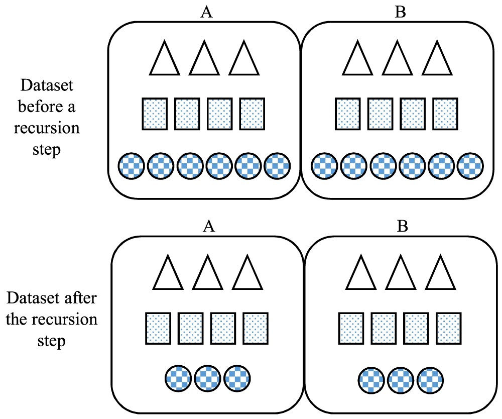
The illustration of the MHL recursion algorithm; data set D is split to subsets A and B, and then, a classifier c_i is trained on A. It captures the dominant pattern, here circles. The trained model can detect the similar pattern in B, that is circles; these form the $c a n d e c i d e$ set and are removed from B. The remaining data in B, that is, the $c a n n o t d e c i d e$ set is combined with A and split again. In each recursion, a model, or a hypothesis, is learned for the current dominant pattern of data. The recursive process continues until no dominant pattern is left, and then, the last model is trained on the remaining samples and the process stops.

3.3. An MHL algorithm

The idea of the algorithm is to divide the data set into two disjoint subsets $s b_{1}$ and $s b_{2}$ such that these two subsets have similar distributions of labels or classes. It learns the major pattern in $s b_{1}$ with classifier c₁ and stores it as model m₁. Then, it partitions $s b_{2}$ based on m₁s performance into two parts can-decide or cannot-decide samples. The subpartition can-decide contains instances where m₁ can predict their labels with confidence, whereas the other subpartition includes those that m₁ is not sure about their classification. Subsets $c a n n o t d e c i d e$ and $s b_{1}$ are merged to yield a new training set. The process is repeated recursively on the new merged set until no further partitioning into can-decide and $c a n n o t d e c i d e$ is possible.

The algorithm consists of two main parts: Trainer and Tester. Trainer gets the training set T₀, a classifier set C, and a desired sensitivity and specificity: $s e n$ and $s p e c$ . During a recursive procedure, Trainer builds regression models, that is, hypotheses, specific for different patterns of data, which are observed in the input training set T₀. It also stores each produced model M along with two thresholds $T_{u p}$ and $T_{d o w n}$ for the Tester part. For every sample evaluated by M with a value $\geq T_{u p}$ , it would be classified as positive while labeled as negative if its evaluation value is $< T_{d o w n}$ . The model M guarantees the desired sensitivity and specificity $s e n$ and $s p e c$ for the can-decide partition. When the evaluation value is between $T_{d o w n}$ and $T_{u p}$ , the model does not classify the sample and it would be added to the $c a n n o t d e c i d e$ set.

3.4. Trainer

Trainer consists of three functions: $S p l i t t e r ()$ , Model_Builder(), and Threshold_Finder(). The pseudocode of these functions are provided in Algorithm 1, Algorithm 2, and Algorithm 3 respectively. The Splitter (D, C) gets a data set D and a set of classifiers C as input. Classifiers are Weka training modules accessible through its application programmable interface. The $S p l i t t e r ()$ function splits the input set D into two subsets A and B by the Stratification method (Thompson, 2012) to maintain the same ratio of positive samples versus negatives in these subsets as it is in D. A and B are disjointing and complement of each other corresponding to D, that is, $A \cup B = D$ . By calling the function $M o d e l B u i l d e r (c_{i}, A, B)$ , the model m_i is built by classifier c_i on data set A. In addition, the function splits B into can-decide and $c a n n o t d e c i d e$ subsets by evaluating m_i on B samples. A is merged with $c a n n o t d e c i d e$ and is returned as $D_{n e w 1}$ , the new training set. Then, the process is recursively repeated on this new set. To avoid any bias toward the way we split the data by the Stratification method: we swap the position of A and B and then repeat the process.

Depending on how high the thresholds $s e n$ and $s p e c$ are chosen, the Model_Builder() function may not be able to build such a model and might not return a new training set. In such a case, it returns the same set as the input training set, indicating that it failed to build the desired model. Given this condition, function $S p l i t t e r ()$ builds a model with c_i on the input training set D and stops.

There are two thresholds associated with each trained model; $T_{u p}$ and $T_{d o w n}$ . The algorithm Threshold_Finder() computes these thresholds such that the model m_i had a given and desired sensitivity and specificity $s e n$ and $s p e c$ . The higher sensitivity and specificity resulted in larger $c a n n o t d e c i d e$ subset in B. We denote the $c a n n o t d e c i d e$ subset as β.

Algorithm 1: Splitter (D, C)
1 foreach classifier $c_{i} \in C$ do
2 Split D into two subsets A and B by the Stratification method;
3 D_new1 = Model_Builder( $c_{i}, A, B$ ); /^* Model m_i is stored as $m_{i_{a}}$ .^*/
4 if $\| D_{n e w 1} \| < \| D \|$ then
5 \| Splitter ( $D_{n e w 1}, C$ )
6 end
7 $D_{n e w 2}$ = Model_Builder(c_i, B, A); /^* Model m_i is stored as $m_{i_{b}}$ . ^*/
8 if $\| D_{n e w 2} \| < \| D \|$ then
9 \| Splitter ( $D_{n e w 2}, C$ );
10 end
11 if $\| D_{n e w 1} \| = = \| D \|$ OR $\| D_{n e w 2} \| = = \| D \|$ then
12 \| train c_i with D, store it as m_i and stop;
13 end
14 end

Algorithm 2: Model_Builder( $c_{i}, s_{a}, s_{b}$ )
1 Train classifier c_i on set s_a, store the trained model as $m_{i_{a}};$
2 Evaluate set s_b by model $m_{i_{a}};$
3 Store the evaluations as a list L_b of $P a i r (< u r i x l i n k : h r e f = ” h t t p : ∕ ∕ s a m p l e . l a b e l ” > s a m p l e . l a b e l < ∕ u r i >, s a m p l e . e v a l u a t i o n);$
4 Pair ( $T_{d o w n}, T_{u p}$ ) = Threshold_Finder( $L_{b}, s e n, s p e c$ ); /^* find T's satisfying sensitivity and specificity. ^*/
5 $β$ = subset of s_b that evaluated as $\geq T_{d o w n}$ and $< T_{u p};$ /^* the $c a n n o t d e c i d e$ subset. ^*/
6 Store the model $m_{i_{a}}$ with ( $T_{d o w n}, T_{u p}$ );
7 Store ( $s_{b} - β$ ) as an ARFF file; /^* $s_{b} - β$ is the $c a n d e c i d e$ subset, store it for further feature analysis. ^*/
8 Return $s_{a} \cup β$ .

Algorithm 3: Threshold_Finder ( $L_{b}, s e n, s p e c$ )
1 $T_{u p}$ = 1, $T_{d o w n}$ = 0;
2 Votes [] = $\emptyset$ _;
3 do
4 foreach pair $p_{i} \in L_{b}$ do
5 if $p_{i} . e v a l u a t i o n \geq T_{u p}$ then
6 \| Votes[p_i] = positive;
7 end
8 if $p_{i} . e v a l u a t i o n < T_{d o w n}$ then
9 \| Votes[p_i] = negative;
10 end
11 end
12 Compute $s e n_{t m p}$ and $s p e c_{t m p}$ for Votes[];
13 if $s e n_{t m p} < s e n$ OR $s p e c_{t m p} < s p e c$ then
14 \| stop and break;
15 end
16 $T_{d o w n} + = Δ$ ; /^* $Δ = 0.05$ ^*/
17 $T_{u p} - = Δ$ ;
18 while $T_{d o w n} < T_{u p}$ ;
19 Return $P a i r (T_{d o w n}, T_{u p})$

3.5. Tester

The Tester procedure loads all model files, m_i's, from the training step into the memory, and when a new and unlabeled sample is given for evaluation, all models examine the sample. If a model evaluates the sample with a value between $T_{d o w n}$ and $T_{u p}$ , then it does not vote, otherwise it votes with confidence as positive if the value is $\geq T_{u p}$ and as negative for the value $< T_{d o w n}$ . Each vote associated with a weight, which is the size of the data set used to build the model. The weighted average of all votes is returned as the final prediction. If all classifiers' evaluation values are between $T_{d o w n}$ and $T_{u p}$ , then it means that there is no vote for the sample and it is predicted with label zero.

4. Results and Discussion

In the training set, there might be several patterns of microRNA targeting, here we denote them symbolically by circles, squares, triangles, and so on, as an example shown in Figure 3. Initially, circles are the dominant pattern. The MHL algorithm divides it into subsets A and B. Classifier c learns circles pattern when it runs over subset A and creates a model for circles, that is, m_c. Evaluating B with m_c divides B into two partitions; samples decidable by m_c, that is, the $c a n d e c i d e$ set, here circles, and samples that m_c is not sure about, called $c a n n o t d e c i d e$ set. Circles are removed from B because we have m_c that can detect them, but the rest of B are not recognizable by m_c so they are added to A to form a new training set. Now, in the new training set, squares are the dominant pattern, and in next recursion step, a model is built for them. This recursion will continue until all patterns are learned or there is no dominant pattern left. In later case, a model for the remaining samples is created by c and recursion stops.

4.1. Comparison with a DL model of microRNA–target duplexes

DL, a.k.a deep neural networks (NN), is a multilayer artificial NN that can learn complex functions and correlations among input variables. It has been used for microRNA target prediction in several recent methods such as miRAW (Pla et al., 2018) and DeepTarget (Lee et al., 2016). To have a fair comparison based on the same training set and test sets, we built our deep neural network with three layers. In the first layer, there are 4 × 22 × 25 = 188 input nodes, where 22 = length of microRNA sequences and 25 = length of target sequences; we used the one-hot-encoding approach (Sujit Pal, 2017) to convert nominal inputs to numerical values to provide input to the network. The second layer, that is, the hidden layer, has the same number of notes as the first layer. The third layer has one node as the output of the network. We used Keras (Chollet et al., 2015) and TensorFlow to implement our DL model and used grid search for the optimum parameter selection. The training set was split into 70% and 30% for training and validation, respectively. The best performance on the validation set was achieved by parameters “ $e p o c h s = 5$ ” and “ $b a t c h s i z e = 100$ .”

4.2. Test of our MHL algorithm

To test the effectiveness of our algorithm, we measure the area under the precision–recall (PR) curve (AUPRC) and the area under the receiver operating characteristic (ROC) curve (AUC). The AUC has been widely used to measure the performance of a binary classifier, and the AUPRC could provide better metrics to compare classifiers on an imbalanced test set (Boyd et al., 2013). A random classifier has AUC = 0.5 and $A U P R C = (N u m b e r o f p o s i t i v e s a m p l e s) ∕ (T o t a l n u m b e r o f s a m p l e s)$ . In our test sets, the ratio of positives to negatives is 1:10; therefore, a random classifier has performance of AUPRC = 1/11. A perfect classifier has AUC = 1 and AUPRC = 1. We compare AUC and AUPRC of different ML models from the Weka package (Witten et al., 2016) with those of our MHL bundle algorithm. The results are shown as PR and ROC curves in Figure 4, and the areas under these curves are shown in Tables 1 and 2; these tables present the comparison results on the human (HSA) and mouse (MMU) test sets, respectively. The columns of the tables are classifier(s) name, AUC and AUPRC of ML models, and parameters sensitivity and specificity, that is, $s e n$ and $s p e c$ for MHL, AUC, and AUPRC of MHL algorithm when the same ML classifier used as underlying model. The last two columns are MHL improvements in terms of AUC and AUPRC.

FIG. 4.

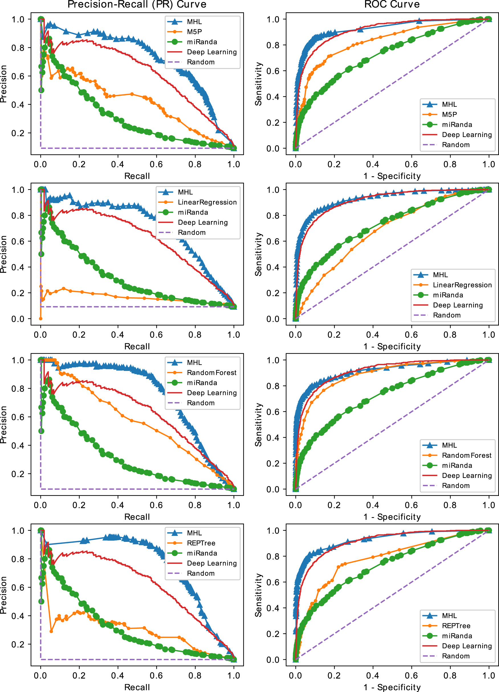
PR and ROC curves of MHL versus ML models, miRanda, a deep learning model and random classifier on HSA (Human) test set. Each row of plots depicts the performance comparisons of MHL versus an ML model in terms of PR and ROC curves. The ML algorithms from the top are M5P, LinearRegression, RandomForest, and REPTree, respectively. The highest improvement due to MHL could be seen in the second row plots when MHL uses LinearRegression as a base classifier. ML, machine learning; PR, precision–recall; ROC, receiver operating characteristic.

Table 1.

The Area Under the Receiver Operating Characteristic Curve and the Area Under the Precision–Recall Curve of Different Machine Learning Models Versus our Multi-Hypotheses Learning Algorithm on HSA (Human) Test Set, $| H S A | = 6129$ Samples

Classifier	AUC	AUPRC	$s e n ∕ s p e c$	MHL-AUC	MHL-AUPRC	AUC improvement	AUPRC improvement
M5P	0.82	0.41	85/85	0.93	0.72	0.11	0.31
LinearRegression	0.68	0.16	85/85	0.93	0.72	0.25	0.56
MultilayerPerceptron	0.64	0.43	85/85	0.83	0.74	0.19	0.31
RandomForest	0.89	0.57	85/85	0.92	0.76	0.03	0.19
REPTree	0.78	0.30	90/90	0.93	0.76	0.15	0.46
DecisionStump	0.57	0.29	85/85	0.75	0.58	0.18	0.29
RandomTree	0.57	0.26	90/90	0.78	0.54	0.21	0.28
miRanda	0.73	0.31
RNAhybrid	0.12	0.05
Deep learning NN	0.91	0.63
Random classifier	0.50	0.09

Each row of the table represents the performance of an ML model versus MHL when MHL used the same module as its underlying classifier. The last two columns show the improvements achieved by MHL. The best performance belongs to MHL when it uses REPTree as its underlying classifier, which yields AUPRC = 0.76 and AUC = 0.93, whereas REPTree by itself has a performance of AUPRC = 0.30 and AUC = 0.78. MHL provides the best performance in all cases except when the underlying classifier is DecisionStump or RandomTree. In these two cases, deep learning NN performs better with AUPRC = 0.63 and AUC = 0.91. The last four rows of the table show performance of miRanda (Betel et al., 2008), RNAhybrid (Rehmsmeier et al., 2004), the deep learning NN, and a random classifier.

AUPRC, area under the precision–recall curve; AUC, area under the receiver operating characteristic curve; MHL, multi-hypotheses learning; ML, machine learning; NN, neural network.

Table 2.

The Area Under the Receiver Operating Characteristic Curve and the Area Under the Precision–Recall Curve of Machine Learning Models Versus Our Multi-Hypotheses Learning Algorithm When They Were Trained on Human and Tested on MMU (Mouse) Test Set, $| M M U | = 517$ Samples

Classifier	AUC	AUPRC	$s e n ∕ s p e c$	MHL-AUC	MHL-AUPRC	AUC improvement	AUPRC improvement
M5P	0.92	0.44	85/85	0.97	0.88	0.05	0.44
LinearRegression	0.54	0.09	85/85	0.99	0.91	0.45	0.82
MultilayerPerceptron	0.73	0.47	85/85	0.97	0.93	0.24	0.46
RandomForest	0.96	0.82	85/85	0.99	0.93	0.03	0.11
REPTree	0.90	0.60	90/90	1.00	0.95	0.10	0.35
DecisionStump	0.49	0.18	85/85	0.61	0.50	0.12	0.32
RandomTree	0.71	0.46	90/90	0.95	0.88	0.24	0.42
miRanda	0.67	0.21
RNAhybrid	0.07	0.05
Deep learning NN	0.97	0.71
Random classifier	0.50	0.09

These tables show that our algorithm is effective, and MHL always achieved a superior performance over ML models. We compare the performances in terms of both AUPRC and AUC. Performance of a binary classifier on balanced data sets is similar in terms of AUPRC and AUC, while in imbalanced test sets, AUPRC is a better determinant of performance. Our test sets have a ratio of 1:10 for positives versus negative samples; therefore, AUPRC values should represent better evaluations for the performance of models.

In Table 1 where models are tested on Human samples, the highest overall performance is achieved by MHL, when it uses REPTree as a base classifier. The model trained by REPTree itself on our training set has a performance of AUC = 0.90 and AUPRC = 0.60. MHL, by using REPTree as base classifier and learning multi-hypotheses, increased the performance to AUC = 0.93 and AUPRC = 0.76. By comparing these measures to those of a random classifier, that is, AUC = 0.50 and AUPRC = 0.09, we can observe that MHL is successful in distinguishing samples that represent a microRNA target from the samples that contain nontargets. The last two columns show improvements achieved by MHL over the base classifiers; the highest improvement in terms of both AUC and AUPRC is when LinearRegression is used as the base classifier.

On our human test set, LinearRegression alone has a mediocre performance with AUC = 0.68 and AUPRC = 0.16. MHL utilized the same classifier to achieve a very high performance with AUC = 0.93 and AUPRC = 0.72. The improvement is 0.25 in AUC and 0.56 in AUPRC. The best performing classifier, trained without MHL, is DL NN with a performance of AUC = 0.91 and AUPRC = 0.71. The second is RandomForest with AUC = 0.89 and AUPRC = 0.57. Classifiers, performing poorly on this test set such as RandomTree and DecisionStump with AUPRCs 0.26 and 0.29, can also be used in MHL to deliver a performance of 0.54 and 0.58. The performance of classifiers alone has an average AUC of 0.71 with a standard deviation 0.13, and an average AUPRC of 0.35 with a standard deviation 0.13. For MHL, the average AUC is 0.87 with a standard deviation of 0.08, and the average AUPRC is 0.69 with a standard deviation of 0.09. MHL increased AUC by 22.53% and AUPRC by 97.14% on average. MHL almost doubled the performance of classifiers in terms of AUPRC. Improvement in AUC is not as high as AUPRC because AUC values for MHL are near perfect with 0.93 for four of the seven classifiers.

We also compare the models trained on our data sets versus two popular algorithms for microRNA target prediction miRanda (Betel et al., 2008) and RNAhybrid (Rehmsmeier et al., 2004). miRanda has an average performance, but RNAhybrid is unable to distinguish targets from nontargets accurately, and that is because miRanda and RNAhybrid are rule-based methods while other models are data-driven. Rule-based methods use microRNA–target duplex stability and its MFE to detect targets. MicroRNA duplexes with noncanonical seeds tend to have higher MFE than duplexes with canonical seeds, due to mismatches in the seed area (Loeb et al., 2012). RNAhybrid uses MFE of the duplex for target recognition, and it does not work well if test set has targets containing noncanonical seeds or has nontargets with relatively low MFE. On the other side, data-driven models could learn more complex correlations between nucleotides in microRNA and target, beyond the MFE and secondary structure of the duplex. This gives an advantage to data-driven models over these rule-based methods.

Table 2 presents the results of training models on Human data and testing on mouse samples. Human and mouse branched from a common ancestor about 80 million years ago. They have similar genomes and virtually the same set of genes (Genome.gov, 2017). Therefore, it is of interest to train a model by human genomic data and test it on mouse data sets. We ran the same model used for testing human data on mouse data set. Our algorithm improves over all ML classifiers, and the maximum improvement again is for Linear Regression with an increase of 0.45 in AUC and 0.82 in AUPRC. The average AUPRC of our algorithm is 0.85 with a standard deviation of 0.16, and for the other ML models that is 0.44 with a standard deviation of 0.25. The MHL algorithm average performance surpasses other ML methods average by 23.43% in AUC and 95.42% in AUPRC.

MHL has similar performance on both mouse and human test sets and that suggests that microRNA–target duplexes and targeting mechanism features are evolutionary conserved across both species. Some microRNAs have conserved sequences among humans and mouse; therefore, there might be a small set of samples with similar sequences in both the (human) training set and the mouse test set. This could be the reason for larger performance improvement on the mouse versus the human test set in Tables 1 and 2, respectively. We reduced the chance of sequence similarity in the human test set by sorting microRNAs and dividing them between training and test sets alternatively with the given ratio of 10:1, and also we subtracted the test set from the training set to avoid any chance of overlaps between the two sets.

Figure 4 shows the PR and ROC curves of our tests. In each row of the figure, there is a pair of plots that show the performance of MHL versus an ML model, miRanda, a DL model and random classifier, when they are evaluated on the human test set. The first row from the top shows performance of M5P ML model versus MHL when it uses M5P as a base classifier. The difference between MHL and M5P curves clearly shows the effectiveness of our algorithm; the M5P curve reflects the performance of the single hypothesis learned by the model, and MHL curve represents the predictive power of several hypotheses learned by MHL. The closest competitor to MHL is the DL model that we trained on our training set. While the performance of the DL model is due to the power of tool and our grid search parameter selection strategy, the superior performance of MHL comes from simulating the structural mechanism of microRNA targeting and also learning hypotheses that model different mechanisms of targeting. Rows 2, 3, and 4 show similar comparisons for MHL versus LinearRegression, RandomForest and REPTree, respectively. The difference in MHL curves, in each row, comes from the different base classifiers that were used within MHL to learn multiple hypotheses. While the performance of ML models varies significantly among themselves, MHL consistently surpassed them and even the powerful DL model by a high margin.

While some data-driven methods, such as RandomForest and DL models have comparable performance with AUC of 0.89 and 0.91, respectively, or GraB-miTarget (Mohebbi et al., 2018), a hybrid model of a graph and a support vector machine, has an AUC performance as high as 0.92, the distinctive advantage of MHL is to provide a clue into the data by partitioning the data into subsets that contain biologically related microRNA duplexes.

4.3. Feature selection analysis of subsets provided by MHL

To check if the samples within subsets provided by MHL have biologically meaningful correlation, we select significant features within each subset and also within the entire training set by using correlation-based feature selection (CFS) algorithm (Hall, 1999), and then, we compare features mined in each subset versus features extracted from the entire training set. From the Weka package, the CFS algorithm was run; the features extracted from the training set and the subsets created by MHL are shown in columns 1 to 6 of Table 3. In our notation for features' name, i is the nucleotide index starting from 1 on 5′ side of a microRNA sequence, and the names are in the format of $i B P$ , $i M i s M a t c h$ , $i B u l g e o n m i c r o R N A$ , or $i B u l g e o n t a r g e t$ . BP composed of two letters X and Y representing a canonical base pair between nucleotides X and Y. For example, $2 A U$ shows a base pair $A - U$ , where A is at index 2 of microRNA and U is in the target sequence. $i M i s M a t c h$ depicts the nucleotide at position i and does not participate in any base pairing. Features $i B o M$ or $i B o T$ represent a bulge at index i on microRNA (M) or target (T), respectively.

Table 3.

Feature Selected by Correlation-Based Feature Selection, from Complete Training Set Versus from Five Subsets Partitioned by the Multi-Hypotheses Learning Algorithm

All training data	Subset 1	Subset 2	Subset 3	Subset 4	Subset 5
2_AU	2_AU	t1_A	2_AU	2_AU	2_AU
2_UA	2_UA	2_AU	2_UA	2_MisMatch	2_UA
2_MisMatch	2_GC	2_UA	3_UA	4_AU	2_GC
3_UA	3_UA	2_GC	4_AU	7_GU	3_UA
4_AU	4_AU	2_MisMatch	4_BoM	8_BoT	4_AU
4_UA	4_UA	2_BoM	5_AU	19_UG	4_UA
4_BoM	4_BoM	3_UA	6_AU	20_AU	4_BoM
5_AU	5_AU	3_BoM	6_UA	20_BoT	5_AU
5_UA	5_UA	4_AU	7_AU	22_AU	5_UA
6_AU	5_BoM	4_UA	8_AU	MFE	6_AU
6_BoM	6_AU	5_UA	8_UA		6_BoM
7_AU	6_BoM	6_AU	9_BoT		7_AU
8_AU	7_AU	6_GU	10_BoT		8_AU
8_UA	7_BoM	7_AU	15_AU		8_UA
10_BoT	8_AU	8_AU	21_UA		10_BoT
15_AU	8_UA	8_UA	22_AU		16_AU
20_AU	13_AU	9_GU	22_GU		20_AU
22_GU	13_GU	10_GU	MFE		20_BoT
MFE	15_AU	16_AU			21_UA
	19_UA	17_UA			MFE
	20_BoT	21_AU
	21_GU	21_UA
	22_AU	22_AU
	MFE	MFE

The comparison of first row with rows 2 to 6 shows that MHL can help to extract biological details from subsets while they could not be captured by the CFS method on the complete training set. In each feature, the number represents the nucleotide index starting from 1 on 5′ side of microRNA. For example, $2 A U$ means adenine in the second position of microRNA pairs to a uracil on the target sequence. In addition, occurrence of bulges on each sides of the microRNA duplex are abbreviated as BoM and BoT, which stand for bulge on microRNA and bulge on target, respectively.

CFS, correlation-based feature selection; MFE, minimum free energy.

In Table 3, column 1, there are several biological details that are missing. The appearance of adenine in the first position of the target, that is, $t 1 A$ , is a major identifier of targets for many human microRNAs M (Witkos et al., 2011). MHL assigned all such samples to subset 2, while $t 1 A$ is missing in column 1 and that indicates that CFS was not able to extract it from the entire training set, but MHL enables us to extract such important feature by clustering all duplex samples with $t 1 A$ into subset 2. Wobble G:U base pairs or single nucleotide bulges have been experimentally verified in the seed area of several microRNAs (Brennecke et al., 2005).

CFS has not been able to extract G:U base pairs from the entire training set, and they are not present in column 1, but with MHL, microRNA duplexes with G:U base pairs have been detected and grouped into subset 4. Column 1 shows that CFS on the entire training data set has been able to detect bulges only in positions 4 and 6, but with MHL, we can detect these bulges in indexes 2, 3, 4, 5, 6, and 7. MicroRNAs with bulges in indexes 2 and 3 are clustered by MHL in subset 2. Subset 4 contains microRNAs with no bulge in the seed area. Subset 1 has microRNAs with bulges in the rear half of the seed, positions 4, 5, and 7. GC is a strong base pair, and a biological mechanism of targeting proposed by Schirle et al. (2014) claims base pairing on positions 2, 3, and 4 make the groove inside Argonaut protein to open and to accommodate the target. MHL has been able to cluster samples related to this mechanism into subsets 1, 2, and 5, while column 1 does not include any GC base pair feature in microRNA duplexes.

The feature $2 m i s m a t c h$ separates canonical seed samples from noncanonicals, and MHL partitioned these two main types of samples into subsets 1, 3, and 5 for canonicals, versus 2 and 4 for noncanonicals. Splitting samples into canonical versus noncanonical subsets has not been explicitly coded into the MHL, but MHL has been able to automatically learn exclusive hypotheses for them and cluster the data accordingly.

Continuous pairing to the 3′ side of microRNA can compensate for single nucleotide bulges or mismatches in the seed region (Bartel, 2009). The first column does not show a significant presence of such pairs, but columns 1 to 4 have continuous base pairs and also have more individual pairs at the 3′ side of microRNA; subsets 1 to 4 contain samples with adjacent pairs at positions 19 to 22. Subset 2, in addition, contains two more continuous base pairs at indexes 16 and 17.

These biologically interpretable details seen in subsets 1 to 5 but missed in column 1 shows that the MHL algorithm can provide subsets of the data that have biologically correlated samples. Samples in these subsets can be further studied or experimented to determine new targeting mechanisms. Based on the current understanding on mechanisms of microRNA targeting, some subsets or features may not have a verified biological interpretation, but they can be used in in vivo experiments to discover new targeting mechanisms.

4.4. Data set clustering of MHL versus standard clustering algorithms

MHL clusters a data set based on a set of optimum hypotheses that it learns through the process of training and that is what makes MHL distinct from standard clustering algorithms. To contrast the clustering merit of MHL versus other standard clustering algorithms, we ran clustering algorithms from the Weka package such as Canopy, Cobweb, Expected Maximization, FarthestFirst, FilteredClusterer, and Xmeans (Witten et al., 2016) on our data set. Table 4 contains these results; column 1 lists algorithms and column 2 shows the number of clusters created by each algorithm. The clustering algorithms from Weka either create too many clusters or splits the data set into two large subsets.

Table 4.

This Table Compares Multi-Hypotheses Learning Clustering Performance Versus Other Standard Algorithms

Clustering algorithm	Number of clusters	Meritscores (weighted average of clusters)
Canopy	100	0.629
Cobweb	917	0.016
EM	15	0.441
FarthestFirst	2	0.56
FilteredClusterer	2	0.51
Xmeans	2	0.51
MHL	5	0.548

We ran these methods from the Weka package, listed in the first column, on our data set. The second column shows the number of clusters created by each algorithm. These algorithms either created too many clusters or split the data set into two large subsets. To evaluate the relevance of samples to each other in a cluster, we then ran the CFS algorithm. If samples in a cluster are relevant, the CFS algorithm gives a high Merit score for the selected features in the cluster. The Merit score is between 0 and 1. For each algorithm, we computed the weighted average of Merit scores for the clusters created by the algorithm, and it is shown in column 3. By comparing columns 2 and 3 for other algorithms versus MHL, one can observe that MHL could give better clusters in terms of the number of subsets and the average Merit score for the subsets.

EM, Expected Maximization.

To see how good is a clustering, we use the Merit score computed by the CFS algorithm for the input data set and for the features it selects. If samples in a cluster are relevant, the CFS algorithm gives a higher Merit score than if the samples are not related. The Merit score is between 0 and 1; a high Merit score means a low correlation between the selected features and a high correlation with the sample label.

For each cluster provided by a clustering algorithm, we ran CFS and used the Merit score as an estimate for the relevance of samples in the cluster. Table 4, column 3, shows the weighted average of Merit scores for each algorithm. We computed the weighted average because the number of clusters created by different algorithms varies. Weight for each cluster score is the proportion of the cluster size to the total number of samples in the training data set. The summation of the weights for each clustering algorithm is one.

Table 4 compares the clustering performance of MHL versus standard clustering algorithms from the Weka package. The results in this table show that MHL clusters better in terms of the number of clusters it creates and the weighted average of Merit scores for the clusters. MHL creates five subsets with an average Merit score of 0.548. The only algorithms with better Merit scores are FarthestFirst with the score 0.56 and Canopy's average score is 0.629. FarthestFirst has a small advantage for the Merit score, but it created two large clusters. Canopy has the highest score, while it created 100 small clusters. MHL is the optimum balance for the number of clusters and the average Merit score.

MHL creates clusters by utilizing the learned hypotheses. For each hypothesis, MHL chooses those samples that the hypothesis could either accept or reject with confidence, a vote close to one or zero, respectively. Other algorithms, however, partition the data set and create clusters based on similarity in attributes' values. Attributes could have different correlations to the label, and this may mislead a clustering algorithm away from partitioning by the most predictive attributes. MHL exhaustively searches for the hypotheses with the highest predictive performance and eventually those optimum ones cluster the data set; thus, MHL created clusters that are biologically meaningful and lead to better predictive performance.

In the last two decades, dozens of algorithms for microRNA target prediction has been published. These methods vary based on the information they use, their accessibility, being rule-based or data-driven, and their fundamentals. For a fair comparison of our method versus state-of-the-art methods, we studied several of the renown tools, such as TargetScan (Agarwal et al., 2015), TarPmiR (Ding et al., 2016), miRBase (Griffiths-Jones et al., 2006), DIANA-microT (Maragkakis et al., 2009), miRanda (Betel et al., 2008), miTarget (Kim et al., 2006), RNAhybrid (Rehmsmeier et al., 2004), Avishkar (Ghoshal et al., 2015), TargetSpy (Sturm et al., 2010), miRWalk (Dweep et al., 2011), and miRanda-mirSVR (Betel et al., 2010).

Some of these algorithms use a variety of other information, in addition to microRNA duplex sequences, for target prediction. For example, TargetScan (Agarwal et al., 2015), miRanda-mirSVR (Betel et al., 2010), and DIANA-microT (Maragkakis et al., 2009) use sequence conservation across species, conserved or nonconserved microRNA family, and miRBase annotation. Our MHL target predictions rely only on sequences of a microRNA duplex. Comparing MHL with methods such as TargetScan would be technically not feasible because our collected data do not have the information used by TargetScan. The other challenge was that the source code or executable files for some methods are not available, and they are only accessible through their online websites, for instance, miRDB (Wang, 2008), miTarget (Kim et al., 2006), and miRWalk (Dweep et al., 2011).

Our test set composed of 6646 samples (HSA 6129 samples and MMU 517), and we could not submit the test set as thousands of online queries manually. The functionality of some of these methods is different from our method, for example, TarPmiR (Ding et al., 2016) finds targets across a given mRNA for a microRNA sequence, whereas our data samples are pairs of short microRNA and target site sequences, and MHL is about finding out if a pair bind to each other. From available software and methods for microRNA target prediction, we could only use those with downloadable source code or executable code. Moreover, for a fair comparison, such methods would also need to predict a microRNA target merely based on sequences of microRNA and target site. Software tools satisfying all these requirements were miRanda (Betel et al., 2008) and RNAhybrid (Rehmsmeier et al., 2004). These rule-based methods work based on fundamental principles of microRNA targeting mechanisms such as a lower free energy binding and a stable secondary structure duplex. These metrics have had reliable performance; therefore, miRanda and RNAhybrid are still widely used either solely or as core components of other algorithms such as miRanda-mirSVR (Betel et al., 2010) and miRanda-MiRBase (Maziere and Enright, 2007).

5. Conclusion

MicroRNAs are small RNA sequences that regulate genes and have important and diverse functions. Biologists are very interested to discover the functionality of microRNAs, and their functions may be correlated with the way they detect their targets. As a result, microRNA studies and specifically microRNA target prediction received a lot of attention, and many computational algorithms have been developed in the last two decades. In this work, we presented a multi-hypotheses learner (MHL) algorithm that aims for two purposes: first, to predict microRNA targets with high accuracy, and second, to help with discovering the mechanisms of microRNA targeting, by providing partitions of samples that biologically correlate with each other within a partition. These partitions can potentially be used for in vivo experiments to discover new mechanisms of microRNAs target recognition.

Our MHL algorithm has significantly improved the performance of some ML methods by correct partitioning of the data set; for example, LinearRegression, MultilayerPerceptron, and REPTree have average performances when they are trained alone on the data set, but MHL boosts their performance to have very high performances and outperform powerful algorithms such as DL models and RandomForest. Feature selection analysis on the partitions created by MHL reveals that the MHL partitioning mechanism is indeed biologically meaningful and partitions have verified features that could not be mined without using the MHL algorithm.

Footnotes

Acknowledgments

The authors would like to thank Dr. Cory Momany and Dr. Khaled Rasheed for their feedbacks and comments on this work.

Author Disclosure Statement

The authors declare they have no competing financial interests.

Funding Information

This work was supported in part by the NIH grant (Award No: R01GM117596), as a part of Joint DMS/NIGMS Initiative to Support Research at the Interface of the Biological and Mathematical Sciences, and NSF IIS grant (Award No: 0916250).

References

Agarwal

, Bell

G.W.

, Nam

J.-W.

, et al. 2015. Predicting effective microRNA target sites in mammalian mRNAs. Elife, 4, e05005.

Bartel

D.P.

2009. MicroRNAs: Target recognition and regulatory functions. Cell, 136, 215–233.

Betel

, Koppal

, Agius

, et al. 2010. Comprehensive modeling of microRNA targets predicts functional non-conserved and non-canonical sites. Genome Biol. 11, R90.

Betel

, Wilson

, Gabow

, et al. 2008. The microrna.org resource: Targets and expression. Nucleic Acids Res. 36(Suppl 1), D149–D153.

Boyd

, Eng

K.H.

, and Page

C.D.

2013. Area under the precision-recall curve: Point estimates and confidence intervals. In Joint European Conference on Machine Learning and Knowledge Discovery in Databases, 451–466. Springer, Berlin-Heidelberg, Germany.

Brennecke

, Stark

, Russell

R.B.

, et al. 2005. Principles of microRNA–target recognition. PLoS Biol. 3, e85.

Chollet

2015. Keras. Available at: https://github.com/fchollet/keras Accessed October 5, 2020.

Cloonan

2015. Re-thinking miRNA-mRNA interactions: Intertwining issues confound target discovery. Bioessays, 37, 379–388.

Ding

, Li

, and Hu

2016. Tarpmir: A new approach for microRNA target site prediction. Bioinformatics, 32, 2768–2775.

10.

Dweep

, Sticht

, Pandey

, et al. 2011. mirwalk–database: Prediction of possible miRNA binding sites by walking the genes of three genomes. J. Biomed. Inform. 44, 839–847.

11.

Enright

A.J.

, John

, Gaul

, et al. 2004. MicroRNA targets in drosophila. Genome Biol. 5, R1.

12.

Friedman

R.C.

, Farh

K.K.-H.

, Burge

C.B.

, et al. 2009. Most mammalian mRNAs are conserved targets of microRNAs. Genome Res. 19, 92–105.

13.

Genome.gov, 2017. Why Mouse Matters. Available at: https://www.genome.gov/10001345 Accessed January 6, 2017.

14.

Ghoshal

, Grama

, Bagchi

, et al. 2015. An ensemble SVM model for the accurate prediction of non-canonical microRNA targets. In Proceedings of the 6th ACM Conference on Bioinformatics, Computational Biology and Health Informatics, 403–412. ACM, New York, New York, USA.

15.

Griffiths-Jones

, Grocock

R.J.

, Van Dongen

, et al. 2006. mirbase: MicroRNA sequences, targets and gene nomenclature. Nucleic Acids Res. 34(Suppl 1), D140–D144.

16.

Hall

M.A.

Correlation-Based Feature Selection for Machine Learning. PhD Thesis, The University of Waikato, 1999.

17.

Hsu

S.-D.

, Tseng

Y.-T.

, Shrestha

, et al. 2014. mirtarbase update 2014: An information resource for experimentally validated miRNA-target interactions. Nucleic Acids Res. 42, D78–D85.

18.

Jansson

M.D.

, and Lund

A.H.

2012. MicroRNA and cancer. Mol. Oncol. 6, 590–610.

19.

John

, Enright

A.J.

, Aravin

, et al. 2004. Human microRNA targets. PLoS Biol. 2, e363.

20.

Kim

S.-K.

, Nam

J.-W.

, Rhee

J.-K.

, et al. 2006. mitarget: MicroRNA target gene prediction using a support vector machine. BMC Bioinformatics, 7, 411.

21.

Kiriakidou

, Nelson

P.T.

, Kouranov

, et al. 2004. A combined computational-experimental approach predicts human microRNA targets. Genes Dev. 18, 1165–1178.

22.

Lee

, Baek

, Park

, et al. 2016. deeptarget: End-to-end learning framework for microRNA target prediction using deep recurrent neural networks. In Proceedings of the 7th ACM International Conference on Bioinformatics, Computational Biology, and Health Informatics, 434–442. New York, New York, USA.

23.

Lewis

B.P.

, Burge

C.B.

, and Bartel

D.P.

2005. Conserved seed pairing, often flanked by adenosines, indicates that thousands of human genes are microRNA targets. Cell, 120, 15–20.

24.

Lewis

B.P.

, Shih

I.-H.

, Jones-Rhoades

M.W.

, et al. 2003. Prediction of mammalian microRNA targets. Cell, 115, 787–798.

25.

Lin

, and Gregory

R.I.

2015. MicroRNA biogenesis pathways in cancer. Nat. Rev. Cancer, 15, 321–333.

26.

Loeb

G.B.

, Khan

A.A.

, Canner

, et al. 2012. Transcriptome-wide mir-155 binding map reveals widespread noncanonical microRNA targeting. Mol. Cell, 48, 760–770.

27.

Lorenz

, Bernhart

S.H.

, Zu Siederdissen

C.H.

, et al. 2011. ViennaRNA package 2.0. Algorithms Mol. Biol. 6, 26.

28.

Maragkakis

, Reczko

, Simossis

V.A.

, et al. 2009. Diana-microt web server: Elucidating microRNA functions through target prediction. Nucleic Acids Res. 37(Suppl 2), W273–W276.

29.

Maziere

, and Enright

A.J.

2007. Prediction of microRNA targets. Drug Discov. Today, 12, 452–458.

30.

Mohebbi

, Ding

, Malmberg

R.L.

, et al. 2018. Accurate prediction of human miRNA targets via graph modeling of miRNA-target duplex. J. Bioinform. Comput. Biol. 16, 850013.

31.

Mohebbi

, Ding

, Malmberg

R.L.

, et al. 2019. A multi-hypothesis learning algorithm for human and mouse miRNA target prediction. In International Conference on Computational Advances in Bio and Medical Sciences, 102–120. Springer, Cham, Switzerland.

32.

Peterson

S.M.

, Thompson

J.A.

, Ufkin

M.L.

, et al. 2014. Common features of microRNA target prediction tools. Front Genet. 5, 23.

33.

Pla

, Zhong

, and Rayner

2018. miraw: A deep learning-based approach to predict microRNA targets by analyzing whole microRNA transcripts. PLoS Comput. Biol. 14, e1006185.

34.

Rehmsmeier

, Steffen

, Höchsmann

, et al. 2004. Fast and Effective Prediction of MicroRNA/Target Duplexes, vol 10. Cold Spring Harbor Lab, Cold Spring Harbor, NY.

35.

Rusinov

, Baev

, Minkov

I.N.

, et al. 2005. Microinspector: A web tool for detection of miRNA binding sites in an RNA sequence. Nucleic Acids Res. 33(Suppl 2), W696–W700.

36.

Schirle

N.T.

, Sheu-Gruttadauria

, and MacRae

I.J.

2014. Structural basis for microRNA targeting. Science, 346, 608–613.

37.

Sturm

, Hackenberg

, Langenberger

, et al. 2010. Targetspy: A supervised machine learning approach for microRNA target prediction. BMC Bioinformatics, 11, 1.

38.

Sujit Pal

A.G

. 2017. Deep Learning with Keras. Packt Publishing, Birmingham, UK.

39.

Thompson

S.K.

2012. Sampling. Wiley, Hoboken, New Jersey, USA.

40.

Wang

2008. mirdb: A microRNA target prediction and functional annotation database with a wiki interface. RNA, 14, 1012–1017.

41.

Weill

, Lisi

, Scott

, et al. 2015. Mirbooking simulates the stoichiometric mode of action of microRNAs. Nucleic Acids Res. 43, 6730–6738.

42.

Witkos

T.M.

, Koscianska

, and Krzyzosiak

W.J.

2011. Practical aspects of microRNA target prediction. Curr. Mol. Med. 11, 93–109.

43.

Witten

I.H.

, Frank

, Hall

M.A.

, et al. 2016. Data Mining: Practical Machine Learning Tools and Techniques. Morgan Kaufmann, Burlington, Massachusetts, USA.

44.

Yue

, Liu

, and Huang

2009. Survey of computational algorithms for microRNA target prediction. Curr. Genomics. 10, 478–492.