Complex Variant Discovery Using Discordant Cluster Normalization

Abstract

Complex genomic structural variants (CGSVs) are abnormalities that present with three or more breakpoints, making their discovery a challenge. The majority of existing algorithms for structural variant detection are only designed to find simple structural variants (SSVs) such as deletions and inversions; they fail to find more complex events such as deletion–inversions or deletion–duplications, for example. In this study, we present an algorithm named CleanBreak that employs a clique partitioning graph-based strategy to identify collections of SSV clusters and then subsequently identifies overlapping SSV clusters to examine the search space of possible CGSVs, choosing the one that is most concordant with local read depth. We evaluated CleanBreak's performance on whole genome simulated data and a real data set from the 1000 Genomes Project. We also compared CleanBreak with another algorithm for CGSV discovery. The results demonstrate CleanBreak's utility as an effective method to discover CGSVs.

1. Introduction

Complex genomic structural variants (CGSVs) are caused by single mutations that result in multiple genomic rearrangement breakpoints. These breakpoints are not adequately explained by events that cause simpler mutations such as basic deletions and insertions (Quinlan and Hall, 2012). CGSVs correspondingly present with three or more breakpoints. Algorithmic discovery of structural variants has important applications in population genetics and medical diagnoses as they are hallmarks of phenotypic variation and cancer progression, for example. Examples of CGSVs include deletion–inversions, duplication–deletions, and inverted duplications, though many more examples exist (Zhao et al., 2016). They are a hallmark of several diseases and disorders such as cancer and autism spectrum disorder (Rausch et al., 2012a; Brand et al., 2015). Other studies note the contribution of CGSVs to Mendelian disorders such as Potocki–Lupski syndrome (Qvarfordt et al., 1998) and MEC2 duplication syndrome (Beck et al., 2015).

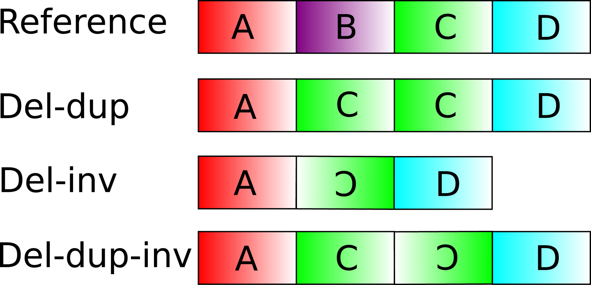
Figure 1 depicts examples of complex structural variants compared with a reference genome. The majority of existing algorithms for structural variant discovery are capable of detecting simple structural variants (SSVs) such as deletions, tandem repeats, and inversions. However, they are unable to accurately detect and classify the complex events depicted in Figure 1. For example, the deletion–inversion case would likely be predicted by these methods as two overlapping inversions. Also, the deletion–duplication case would likely cause the deletion of segment B to be missed by an algorithm that performs SSV discovery using only abnormally mapped read pairs. Accurately discovering and classifying CGSVs require the application of algorithms that are specifically designed to detect these features.

FIG. 1.

Examples of complex genomic structural variants compared with a reference genome. Since the constituent structural variants are consecutive, algorithms to find simple structural variants will likely fail to accurately classify them. This figure is inspired by figure 1 from Zhao et al. (2016).

In this study, we present an algorithm named CleanBreak that discovers CGSVs using mapped Illumina paired reads. The method first employs a graph-based algorithm to cluster all homogeneous read pairs, where each cluster is a possible SSV. The method then collects groups of overlapping SSV coordinates (indicative of a CGSV) and classifies each overlapping group as a CGSV, recursively “normalizing” discordant read pairs until a final set of variants is determined. The predicted CGSV is the one that is the most concordant with local read depth.

Regarding other methods, the CouGaR algorithm is designed to find complex genomic variants in cancer genomes, specifically those variants that cause highly amplified genomic segments connected by SSV breakpoints (e.g., signatures of double minute chromosomes) (Dzamba et al., 2017). With the CouGaR algorithm, the identification of complex genomic arrangements, the prediction of cellular structural level, and the determination of the amount of copies in a tumor genome using whole genome sequencing are possible by employing a five-step algorithm: (1) generating a list of tumor adjacencies, (2) identifying amplified regions, (3) constructing a tumor adjacency graph, (4) counting the number of copies, and (5) predicting circular and linear contigs. SVelter (Zhao et al., 2016) is another algorithm for CGSV discovery. This algorithm first collects groups of discordantly mapped read pairs, that is, those that indicate a likely variant. It then employs a randomized and probabilistic approach by assuming that an initial configuration of overlapping read pairs is explained by a randomly chosen underlying set of SSVs. The method then iteratively improves this prediction by rearranging consecutive blocks of genomic intervals separated by breakpoints. It performs this rearrangement until it converges to an underlying structure that is most consistent with local read depth, read orientation, and read pair insert size.

2. Methods

2.1. Clustering of discordant read pairs

CleanBreak takes as input a set of aligned paired reads in binary sequence alignment/map (SAM) format (Li et al., 2009). In the first step, it collects clusters of overlapping, homogeneous read pairs that could indicate a likely structural variant breakpoint. These read pairs, also known as discordant read pairs, are aligned to the reference genome with characteristics that deviate from the expected library insert size and/or read orientation. These aberrant read alignments could indicate a possible variant. The following are typical discordant read pair alignments and the SSVs they usually imply (assuming Illumina sequencing): 1.

Both reads map with forward–forward or reverse–reverse orientation (inversion type).

The leftmost read maps with reverse orientation, but the rightmost read maps with forward orientation (tandem duplication type).

The relative orientation of the mapped reads is correct, but the distance between the reads is significantly larger than the library insert size (deletion type).

The relative orientation of the reads is correct, but the distance between the reads is smaller than the library insert size (insertion type).

The reads in a single pair map to different chromosomes (interchromosomal rearrangement type).

In parentheses are the SSVs that are typically supported by these discordant alignments. The problem is much more complex for CGSVs, however. Thus, the mentioned discordant alignments will not necessarily indicate the given simple variant type for the problem of CGSV detection. CleanBreak recognizes types 1–3 since insertions are difficult to detect with the paired end strategy.*

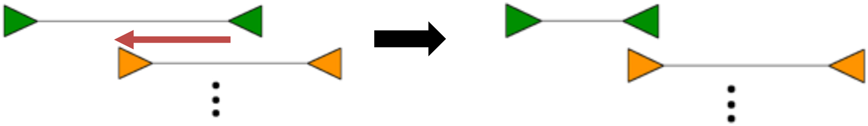
To collect these clusters of discordant read pairs, the method creates an undirected graph where nodes are discordant read pairs and edges connect vertices if the read pairs have overlapping mapping coordinates. Figure 2 illustrates the conversion of a discordant read pair cluster into an undirected graph. Furthermore, the absolute difference of mapping coordinates between two discordant read pairs is assigned as the weight for each edge.

FIG. 2.

Overlapping discordant read pairs mapped to a reference genome and the corresponding graph they induce.

Owing to sequence homology on the reference genome, overlapping variants on separate haplotypes, and complex structural variants, it is possible for multiple clusters to have overlapping coordinates. Individual clusters are resolved by partitioning each connected component in the graph into a set of minimal weight cliques. Since partitioning an undirected graph into minimum weight cliques is computationally difficult (NP-hard), we apply a greedy heuristic that performs this task quickly. This process helps to ensure that read pairs with proximal start and end positions (indicative of the same variant) are grouped together in the same cluster. In Figure 2, the blue discordant read pairs form a cluster, whereas the green pairs form an overlapping, but separate cluster. Despite the fact that the blue and green pairs overlap, they do not support the same variant and should thus be grouped separately. CleanBreak's clique partitioning heuristic addresses this task. Clique finding during the clustering phase is common to algorithms such as Delly (Rausch et al., 2012b) and CLEVER (Marschall et al., 2012), although these methods are designed to discover SSVs.

2.2. CleanBreak algorithm

The algorithm collects cluster coordinates identified in the previous cluster-resolution step. Afterward, it extracts clusters with overlapping coordinates, which is indicative of a possible CGSV. The method predicts complex variants by attempting to “normalize” the predicted cluster coordinates—it attempts to reverse the orientation and distance of predicted clusters if it deviates from the default library settings. Starting with consecutive overlapping clusters, the method performs this normalization until it predicts the CGSV that is the most concordant with local read depth. The reason for this process is that SSV prediction relies on identifying the canonical discordant read pair signals that support deletions, inversions, and tandem repeats. However, since CGSVs essentially comprise several adjoining SSV breakpoints, the appearance of these signals near CGSV breakpoints does not necessarily indicate their respective simple variant. For example, the deletion–inversion case in Figure 10 does not show a forward–reverse cluster with larger-than-normal mapping distance (indicative of a simple deletion). This is because the deletion is adjacent to an inverted segment that obfuscates the expected signal. In other words, for complex variants, the apparent discordant pair signal does not necessarily imply the presence of its corresponding SSV. CleanBreak addresses this issue by exhaustively applying the following rules, each of which are specific to each variant type.

2.2.1. Deletion normalization: rule D1

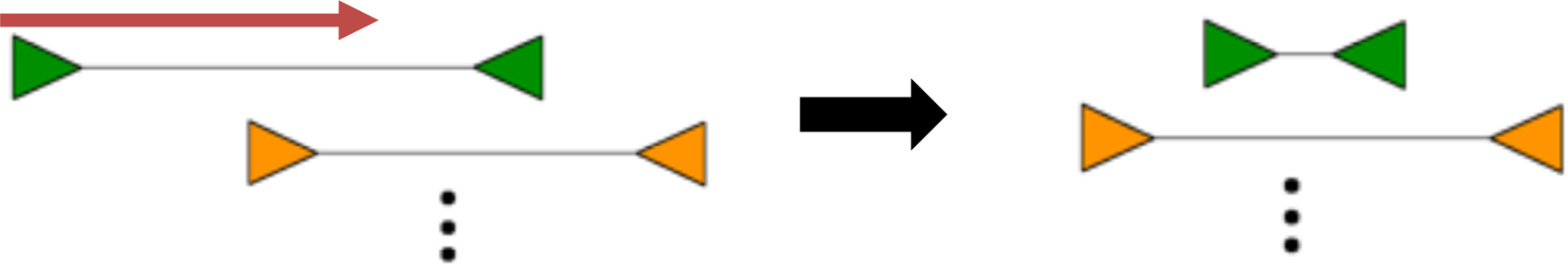
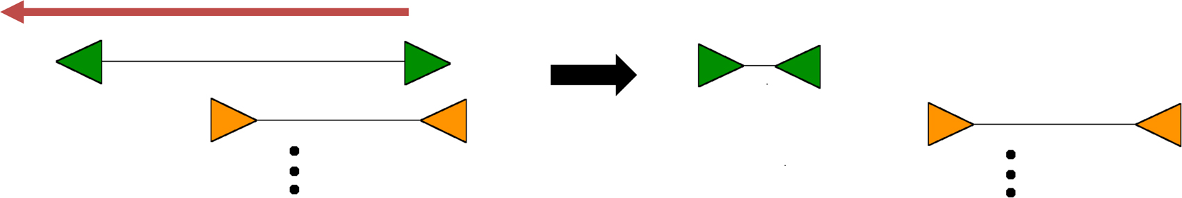
The first rule for deletion normalization is illustrated in Figure 3. The green and orange intervals are the predicted cluster intervals and the orientation of their left and right boundaries.^† This normalization rule requires that the leftmost boundary of the first cluster be moved to the coordinate of the leftmost boundary of the second cluster because it assumes that the interval between these leftmost boundaries is a potential deletion. However, it is not predicted as such unless it is highly concordant with local read depth (the algorithm is explained in Section 2.2.9).

FIG. 3.

Normalization rule D1. The green and orange clusters have overlapping coordinates. This normalization step assumes that the distance between the leftmost cluster boundaries is a deletion. The first cluster's coordinates are updated accordingly.

2.2.2. Deletion normalization: rule D2

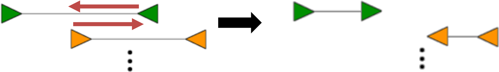
The second rule for deletion normalization is illustrated in Figure 4. This rule assumes that the deletion is between leftmost coordinate of the orange cluster and the rightmost coordinate of the green cluster. Furthermore, the position of the rightmost green boundary is moved to the same position as the leftmost orange boundary.

FIG. 4.

Normalization rule D2.

2.2.3. Deletion normalization: rule D3

The third rule for deletion normalization is illustrated in Figure 5. This rule assumes that a deletion spans the interval of the first cluster in an overlapping pair (the green cluster in Fig. 5). For this rule, the cluster is normalized by adjusting the start position of the leftmost coordinate of the first cluster; it is adjusted to a position that is near the rightmost coordinate of the cluster, approximately within $m + k σ$ , where m is the median mapped distance of read pairs, $σ$ is the median absolute deviation of mapped distances, and k is a user-defined constant (typically between 4 and 6).

FIG. 5.

Normalization rule D3.

2.2.4. Deletion normalization: rule D4

The fourth rule for deletion normalization is illustrated in Figure 6. This rule is similar to rule D3—it assumes that a deletion spans the interval of the first cluster in an overlapping pair. However, this rule normalizes the cluster by adjusting the rightmost boundary in the first cluster—it moves it upstream near the left boundary, within $m + k σ$ base pairs as described for rule D3.

FIG. 6.

Normalization rule D4.

2.2.5. Inversion normalization: rule I1

There are two rules for inversion normalization. The first rule, I1, assumes that the interval between the left boundaries of two overlapping clusters is an inversion. This is illustrated in Figure 7. The left boundaries of both clusters are adjusted as shown in this figure. Furthermore, the orientations of the left boundaries are inverted to account for the possible inversion within the interval.

FIG. 7.

Normalization rule I1.

2.2.6. Inversion normalization: rule I2

The second rule, I2, assumes that the interval between the right boundary of the first cluster and the left boundary of the second cluster is an inversion. This is illustrated in Figure 8. The right boundary of the first cluster is adjusted to the original position of the left boundary of the second cluster. Also, the left boundary of the second cluster is adjusted to the original position of the first cluster's right boundary. The orientations of these cluster boundaries are also inverted to account for the possible inversion event.

FIG. 8.

Normalization rule I2.

2.2.7. Tandem repeat normalization: rule T1

A complex variant interval could be subject to a tandem repeat. This possibility is accounted for by rule T1. For consecutive overlapping clusters, this rule moves the right boundary of the first cluster to a region upstream of its left boundary. This region is within $m + k σ$ base pairs. Thus, this rule assumes that the entire region spanned by the first cluster interval is generated by a segmental duplication. The normalization rule is depicted in Figure 9.

FIG. 9.

Normalization rule T1.

2.2.8. Concordance score algorithms

CleanBreak recursively applies all of the aforementioned rules to the cluster intervals until no more normalization moves are possible. It chooses the normalization path that is the most consistent with local read depth. For each of the normalized intervals depicted by the red arrows, the method computes concordance scores whose values depend on local read depth—the precise value of the concordance score depends on the variant under consideration. For example, a region that supports a tandem repeat should have a high concordance score if local read depth is higher than the genome-wide read depth. A region that supports a deletion should have a high score if local read depth is less than genome-wide read depth. Lastly, a region that supports an inversion should have a high score if local read depth is roughly equal to genome-wide read depth. The algorithms for computing the concordance scores for each type are given in the following algorithms.

Algorithm 1 Algorithm to compute deletion concordance score of interval [A,B]

Input: A genomic interval defined by coordinates A and B.

Output: A real number representing the deletion concordance score of the genomic interval [A,B]

1: procedure concordanceDel (

A, B

)

2: if

r e a d D e p t h ([A, B]) \geq r e a d D e p t h (g e n o m e)

then

s \leftarrow 1

4: else

s \leftarrow | l o g (1 - {(\frac{r e a d D e p t h ([A, B])}{r e a d D e p t h (g e n o m e)})}^{2}) |

6: end if

7: return

1 - s

8: end procedure

Algorithm 2 Algorithm to compute tandem duplication concordance score of interval [A,B]

Input: A genomic interval defined by coordinates A and B.

Output: A real number representing the tandem duplication concordance score of the genomic interval [A,B]

1: procedure concordanceTand (

A, B

)

2: if

r e a d D e p t h ([A, B]) < r e a d D e p t h (g e n o m e)

_then

s \leftarrow 1

4: else

s \leftarrow | \log (1 - {(\frac{r e a d D e p t h (g e n o m e)}{r e a d D e p t h ([A, B])})}^{2}) |

6: end if

7: return

1 - s

8: end procedure

Algorithm 3 Algorithm to compute the inversion concordance score of interval [A,B]

Input: A genomic interval defined by coordinates A and B.

Output: A real number representing the inversion concordance score of the genomic interval [A,B]

1: procedure concordanceInv (

A, B

)

2: if

r e a d D e p t h ([A, B]) = r e a d D e p t h (g e n o m e)

then

s \leftarrow 0

4: else

s \leftarrow | \log (\frac{m i n (r e a d D e p t h (g e n o m e), r e a d D e p t h ([A, B]))}{m a x (r e a d D e p t h (g e n o m e), r e a d D e p t h ([A, B]))}) |

6: end if

7: return

1 - s

8: end procedure

For the concordanceDel algorithm, the score it computes is inversely proportional to the ratio of average genome read depth to the read depth of the genomic interval $[A, B]$ , which is expected if the interval truly represents a genomic deletion. The concordanceTand algorithm is the opposite—the score it returns is directly proportional to the ratio of the interval's read depth to the average read depth of the genome. This is expected since it implies that the read depth in the interval is greater than the entire genome's read depth. The concordanceInv algorithm computes the concordance score for the interval $[A, B]$ assuming that the interval represents an inversion. Since inversions are copy-neutral events, the score returned by this algorithm is highest when the ratio of the average genomic read depth to the interval read depth is closest to 1.

2.2.9. Main algorithm

Having defined the concordance score algorithms, we can define the CleanBreak algorithm as follows:

Algorithm 4 Algorithm to predict complex structural variant coordinates

procedure CleanBreak(C)

if i = n then

return

c o n c o r d a n c e (C i)

▹ Concordance function depends on how the interval is classified

else

R e c o r d R u l e D 1 (C i, C i + 1)

m₁ =

c o n c o r d a n c e D e l (l e f t (C i), l e f t (C i + 1))

C l e a n B r e a k (C i + 1)

R e c o r d R u l e D 2 (C i, C i + 1)

m₂ =

c o n c o r d a n c e D e l (r i g h t (C i), l e f t (C i + 1))

C l e a n B r e a k (C i + 1)

R e c o r d R u l e D 3 (C i)

10: m₃ =

c o n c o r d a n c e D e l (l e f t (C i)

r i g h t (C i)

−

m e d I n s e r t S i z e)

C l e a n B r e a k (C i + 1)

R e c o r d R u l e D 4 (C i)

m₄ =

c o n c o r d a n c e D e l (l e f t (C i), l e f t (C i + 1

m e d I n s e r t S i z e)

C l e a n B r e a k (C i + 1)

R e c o r d R u l e I 1 (C i, C i + 1)

m₅ =

c o n c o r d a n c e I n v (l e f t (C i), l e f t (C i + 1))

C l e a n B r e a k (C i + 1)

15:

R e c o r d R u l e I 2 (C i, C i + 1)

m₆ =

c o n c o r d a n c e I n v (l e f t (C i + 1), r i g h t (C i))

C l e a n B r e a k (C i + 1)

R e c o r d R u l e T 1 (C i)

m₇ =

c o n c o r d a n c e T a n d (l e f t (C i) - m e d I n s e r t S i z e, r i g h t (C i))

C l e a n B r e a k (C i + 1)

return

m a x (m 1, m 2, m 3, m 4, m 5, m 6, m 7)

20: ▹ Predicted variant is the one on the interval that maximizes total score

end if

end procedure

The input C is a set of predicted clusters that form a single connected component in the cluster graph (Fig. 2). Such an input is a candidate complex structural variant. The left and right functions return the left and right genomic coordinates of their input component C, respectively. The RecordRule functions keep track of the candidate variant that spans the given interval.^‡ The algorithm applies each rule previously defined and recursively repeats this process for the remaining cluster components after the concordance scores have been tallied. Once the algorithm reaches the last cluster interval (i.e., the interval that does not precede a consecutive overlapping interval), it predicts the variant based only on the length of the interval and the orientation of its interval boundaries.^§

Beginning with the cluster with the leftmost coordinate position, for each cluster interval in an overlapping component, CleanBreak recursively searches the space of possible variants that can explain the observed clusters. Figure 10 illustrates this process for a possible deletion–inversion complex variant. In this example, the method adjusts the leftmost coordinate of the blue cluster to account for a possible deletion since this will ostensibly be the best choice according to local read depth. After making this choice, the method adjusts the rightmost coordinate of the blue cluster and the leftmost coordinate of the black cluster. This move will also change the orientation of these coordinates that corresponds to an inversion event. Once again, multiple cluster choices are considered during this process, but the choices in the figure are the optimal choices. CleanBreak records the optimal choice made at each step (deletion–inversion in this case), and it terminates when there are no more cluster breakpoints to resolve. The definition of the “optimal” choice is that which maximizes the total concordance score for the component, as determined by Algorithms 1–3. Since CleanBreak exhaustively searches all possible intervals between cluster boundaries, we expect that it at least approximates the globally optimal solution, given the concordance scores defined in Algorithms 1–3.

FIG. 10.

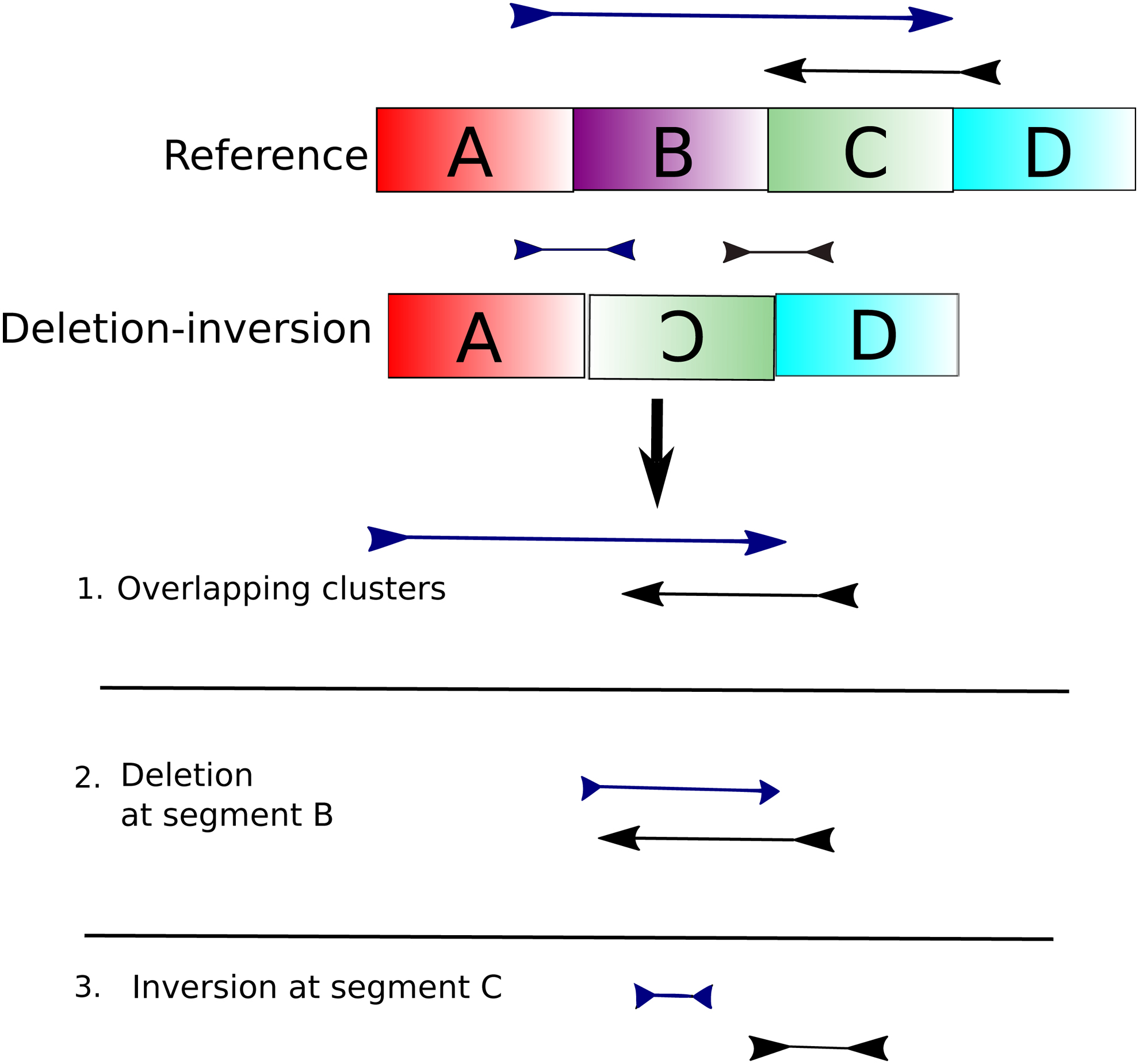
Deletion–inversion, the likely clusters that would result after read mapping, and the likely steps that would be taken by CleanBreak to predict the complex deletion and complex inversion.

3. Results

3.1. Complex variant discovery in simulated data

Simulated paired read data sets were created that consisted of 3000 total complex structural variants (SVs) on chromosome 1 of the human reference genome build hg38. Three separate data sets were created, containing 1000 deletion–duplications, 1000 deletion–inversions, and 1000 deletion–duplication–inversions. These variants were inserted into the reference using SVsim (Faust, 2015). Subsequently, WGSim was used to generate the paired reads (Li, 2011). This data set consisted of 150 bp reads with 400 bp fragments (standard deviation of 70) and ∼80 × mapped read coverage once aligned to the reference with Burrows-Wheeler Aligner (BWA) (Li and Durbin, 2010). CleanBreak was evaluated on its ability to accurately detect deletions, inversions, and tandem repeats that are within the breakpoints of the aforementioned complex variants. The sensitivity of predictions is the percentage of true complex SV breakpoints predicted by the method. A predicted variant overlaps the known variant if there is at least 70% reciprocal overlap between their coordinates. The positive predictive value (PPV) is measured as the percentage of type-specific predictions that overlap the true coordinate locations. Interval overlaps were computed using the Intersect program of the BEDTools suite (Quinlan and Hall, 2010). For comparison, we executed SVelter's on these data sets as well and measured sensitivity and PPV using the mentioned definitions. For SVelter, default parameters were used.

The results of the sensitivity/PPV analysis are provided in Table 1. A comparison of execution times on these data sets is provided in Table 2.

Table 1.

Sensitivity/Positive Predictive Value of Predictions: SVelter Versus CleanBreak (Percentages Out of 1000 Variants)

Algorithm	SV type	Del-Dup	Del-Inv	Del-Dup-Inv
CleanBreak	Del	0.81/0.99	0.73/0.96	0.38/0.38
	Inv	—	0.74/0.90	<0.05/<0.05
	Tand. dup.	0.73/0.97	—	0.26/0.96
SVelter	Del	0.70/0.99	0.66/0.98	0.48/0.96
	Inv	—	0.48/0.97	0.33/0.95
	Tand. dup.	0.54/0.98	—	0.30/0.82

SVs, structural variants.

Table 2.

Simulated Data Running Time Comparison: SVelter Versus CleanBreak

Algorithm	Data set	Time
CleanBreak	Del-Dup	1 h 23 min
	Del-Inv	1 h 15 min
	Del-Dup-Inv	1 h 47 min
SVelter	Del-Dup	1 h 45 min
	Del-Inv	1 h 29 min
	Del-Dup-Inv	2 h 22 min

The data sets were executed on an 8-node cluster with 40 cores/node, 2.1 GHz processors, and 64 GB of RAM.

3.2. Deletion prediction in NA12878

We also evaluated the CleanBreak algorithm to the 30 × coverage downsampled BAM file of a well-characterized genome NA12878, acquired from NIST's Genome in a Bottle Consortium (GIAB) (Genome in a Bottle Consortium, 2012). Using the Picard suite (Broad Institute, 2019), the median insert size and median absolute deviations were estimated to be 552 and 99, respectively. An accompanying list of large benchmarked deletion calls from this set was acquired; these deletions were identified by GIAB using their svclassify framework (Parikh et al., 2016). Using this list of deletions as ground truth, we measured sensitivity and PPV of predicted calls as defined previously for the simulated data, except that we compared results on (1) the original list of benchmarked deletions, (2) only deletions that were ≥1000 bp in the benchmarked data and in the predictions for CleanBreak and SVelter, (3) only deletions that were ≥2000 bp in the benchmarked data and in the CleanBreak and SVelter predictions, and only deletions ≥5000 bp. Evaluating the methods against larger variants was performed to assess the ability of each method to call variants of varying sizes, especially since CleanBreak is designed to find large complex variant intervals.

The results of the comparison are provided in Table 3.

Table 3.

Sensitivity and Positive Predictive Value Comparison on NA12878

Algorithm	SE/PPV (all)	SE/PPV (≥1000 nt)	SE/PPV (≥2000 nt)	SE/PPV (≥5000 nt)
CleanBreak	0.30/0.04	0.89/0.53	0.90/0.60	0.87/0.52
SVelter	0.69/0/55	0.77/0.75	0.75/0.80	0.74/0.75
Total true deletions	2,676	612	408	174

PPV, positive predictive value; SE, sensitivity.

4. Discussion

As suggested by the results on the simulated data, CleanBreak is most accurate in calling deletion–duplication and deletion–inversion events. These are easier events for CleanBreak to handle since there is a 1-to-1 mapping of structural variants to genomic intervals. For this reason, however, the del-dup-inv data set was very difficult for the algorithm to resolve. Nearly all inversion events were misclassified in these data since the vast majority of duplications and inversions shared the same coordinates; in its current state, CleanBreak only assumes one variant per coordinate interval. Furthermore, it is not yet capable of detecting dispersed duplications although there were no such events in the simulated data. However, CleanBreak was faster than SVelter on the simulated data and had higher sensitivity; the PPV was only slightly lower than SVelter. For the Del-Dup and Del-Inv cases, the loss of sensitivity was largely due to the presence of variants within low-complexity regions.

The NA12878 genome has many more ground-truth deletions than other structural variants. Moreover, CleanBreak achieved the greatest sensitivity on predicting larger structural variants. SVelter had a lower false discovery rate overall on these data for all deletion sizes. However, CleanBreak was faster than SVelter on these data, requiring ∼3 days to analyze these data, compared with 4 days and 9 hours for SVelter.

5. Conclusion

We have presented a method to identify complex structural variants using Illumina paired sequencing reads. The method showed the ability to accurately identify variants within deletion–duplication and deletion–inversion events. CleanBreak is currently well suited to discover complex rearrangements whose breakpoints are affected by just a single variant. Simulated data set results support this assertion.

The method is currently limited to intrachromosomal structural variants; it must be adjusted to account for CGSVs involving translocations and other interchromosomal variants. Furthermore, the method may fail to accurately detect dispersed duplications and multiple variants that span the same interval (such as inverted duplications). This largely explains the extremely low sensitivity and PPV for the deletion–duplication–inversion events. These limitations will be the subject of future work. The method will also be extended to account for interchromosomal rearrangements such as translocations. It will also be optimized for applicability to cancer data sets that will require having it distinguished between CGSVs and SSVs shared by many clones/haplotypes. Such an enhancement will require updating the method to have it account for tumor impurity when making predictions.

The CleanBreak software is available here: http://github.com/mhayes20/CleanBreak

Footnotes

Acknowledgment

We thank Dr. Nawa Raj Pokhrel of the Xavier University of Louisiana Department of Physics and Computer Science for helpful discussions.

Disclaimer

This publication was made possible by the Louisiana Cancer Research Consortium. The contents are solely the responsibility of the authors and do not necessarily represent the official views of the NIMHD.

Author Disclosure Statement

The authors declare they have no conflicting financial interests.

Funding Information

This study was partially supported by NSF grant HRD-1901258. This study was also partially supported by NIH-NIGMS grant R25GM060926. Furthermore, support was provided from funding from the NIMHD-RCMI Grant No. 5G12MD007595 from the National Institute on Minority Health and Health Disparities and the NIGMS-BUILD Grant No. 8UL1GM118967.

References

Beck

C.R.

, Carvalho

C.M.

, Banser

, et al. 2015. Complex genomic rearrangements at the PLP1 locus include triplication and quadruplication. PLoS Genet. 11, e1005050.

Brand

, Collins

R.L.

, Hanscom

, et al. 2015. Paired-duplication signatures mark cryptic inversions and other complex structural variation. Am. J. Hum. Genet. 97, 170–176.

Broad Institute. 2019. Picard toolkit. Available at: http://broadinstitute.github.io/picard. Accessed June 8, 2020.

Dzamba

, Ramani

A.K.

, Buczkowicz

, et al. 2017. Identification of complex genomic rearrangements in cancers using CouGaR. Genome Res. 27, 107–117.

Faust

2015. SVsim. Available at: https://github.com/GregoryFaust/SVsim. Accessed June 8, 2020.

Genome in a Bottle Consortium. 2012. Available at: http://jimb.stanford.edu/giab. Accessed June 5, 2020.

2011. WGsim. Available at: https://github.com/lh3/wgsim. Accessed June 8, 2020.

, and Durbin

2010. Fast and accurate long-read alignment with Burrows-Wheeler transform. Bioinformatics, 26, 589–595.

, Handsaker

, Wysoker

, et al. 2009. The Sequence Alignment/Map format and SAMtools. Bioinformatics, 25, 2078–2079.

10.

Marschall

, Costa

I.G.

, Canzar

, et al. 2012. CLEVER: clique-enumerating variant finder. Bioinformatics, 28, 2875–2882.

11.

Parikh

, Mohiyuddin

, Lam

H.Y.

, et al. 2016. svclassify: a method to establish benchmark structural variant calls. BMC Genomics, 17, 64.

12.

Quinlan

A.R.

, and Hall

I.M.

2010. BEDTools: a flexible suite of utilities for comparing genomic features. Bioinformatics, 26, 841–842.

13.

Quinlan

A.R.

, and Hall

I.M.

2012. Characterizing complex structural variation in germline and somatic genomes. Trends Genet. 28, 43–53.

14.

Qvarfordt

, Riise

G.C.

, Larsson

, et al. 1998. Immunological findings in blood and bronchoalveolar lavage fluid in chronic bronchitis patients with recurrent infectious exacerbations. Eur. Respir. J. 11, 46–54.

15.

Rausch

, Jones

D.T.

, Zapatka

, et al. 2012a. Genome sequencing of pediatric medulloblastoma links catastrophic DNA rearrangements with TP53 mutations. Cell, 148, 59–71.

16.

Rausch

, Zichner

, Schlattl

, et al. 2012b. DELLY: structural variant discovery by integrated paired-end and split-read analysis. Bioinformatics, 28, i333–i339.

17.

Zhao

, Emery

S.B.

, Myers

, et al. 2016. Resolving complex structural genomic rearrangements using a randomized approach. Genome Biol. 17, 126.