Parameter Identifiability for a Profile Mixture Model of Protein Evolution

Abstract

A profile mixture (PM) model is a model of protein evolution, describing sequence data in which sites are assumed to follow many related substitution processes on a single evolutionary tree. The processes depend, in part, on different amino acid distributions, or profiles, varying over sites in aligned sequences. A fundamental question for any stochastic model, which must be answered positively to justify model-based inference, is whether the parameters are identifiable from the probability distribution they determine. Here, using algebraic methods, we show that a PM model has identifiable parameters under circumstances in which it is likely to be used for empirical analyses. In particular, for a tree relating 9 or more taxa, both the tree topology and all numerical parameters are generically identifiable when the number of profiles is less than 74.

1. Introduction

A profile mixture (PM) model is a particular stochastic model of protein sequence evolution that describes the changes in sequences along the tree of evolutionary relationships for a collection of taxa. Such a model is often used for the inference of a tree from sequence data, using standard maximum likelihood or Bayesian statistical frameworks. Here we investigate the question of parameter identifiability for this model: Are the model parameters—both the tree topology and numerical parameters—determined by a site pattern distribution arising from the model? Parameter identifiability, which informally means that valid parameter inference is possible in ideal circumstances, is an essential component of the theoretical justification for standard statistical inference approaches.

In models of protein sequence generation, amino acid site patterns are generally assumed to be independent and identically distributed across the sites. Common continuous time models of amino acid substitutions are instances of the general time-reversible (GTR) model, which assumes a single rate matrix Q constant over a metric tree, or extensions that allow for additional scalar rate variation at individual sites. The rate matrix Q has off-diagonal entries from $R d i a g$ (π), where R is a symmetric matrix of exchangeabilities and π is a vector of frequencies of the amino acids that remains stable under the model.

In principle, one can infer R,π, and a metric tree of taxon relationships from protein sequence data using standard statistical frameworks. However, with 20 amino acids, the state space for the model is large, so an exchangeability matrix R is often fixed in advance, having been previously determined empirically for particular types of data. Well-known exchangeabilities for protein alignments include the JTT (Jones et al., 1992), WAG (Whelan & Goldman, 2001), and LG (Le et al., 2008) matrices.

When inspecting protein sequence data, however, it is often clear that the GTR assumption of identically distributed sites is a poor one, since sites have visibly different amino acid compositions. Site residue distributions, or profiles, likely differ because of the biophysical properties of amino acids (e.g., hydrophilia, polarity, or charge), and the associated structural and functional constraints on the protein. This phenomenon suggests a model with multiple classes of substitution processes, and in particular, a mixture model using a variety of profiles with the same exchangeabilities for all classes. Mixture models can provide better fit to data as they introduce more parameters, although they also increase computational time and may lead to overfitting of the data.

However, a more fundamental issue with adopting a mixture model is that one may lose parameter identifiability. If several choices, or even more worrisome, infinitely many choices of parameters lead to the same probability distribution under the model, then even with an idealized infinite data set perfectly in accordance with the model, one could not recover the parameter values under which the data arose. Since the goal of most phylogenetic analyses is to infer model parameters—generally the topological tree but often numerical parameters in addition—identifiability is an essential property for a model to be useful. Nonidentifiability poses particular challenges in Bayesian Markov chain Monte Carlo (MCMC) analyses, where it may be manifested as a lack of convergence (Rannala, 2002).

Parameter identifiability has long been established for nonmixture site substitution models in phylogenetics, but mixture models provide greater challenges. Although computational work may suggest whether it holds or fails, parameter identifiability can only be established theoretically as it is a model property, and not dependent on an inference method. In recent years, algebraic methods have been introduced and successfully applied to a number of phylogenetic mixture models (Allman and Rhodes, 2006, 2008, 2009; Allman et al., 2010, 2011, 2019; Chifman and Kubatko, 2015; Long and Sullivant, 2015; Hollering and Sullivant, 2019; Wascher and Kubatko, 2021). While one of these works (Rhodes and Sullivant, 2012) established a rather general result on parameter identifiability of phylogenetic mixture models with many components, it unfortunately does not apply to the PM model's specific structure.

In this work, we prove parameter identifiability for a PM model of amino acid site substitution. PM models were introduced in the Bayesian context (Lartillot and Philippe, 2004; Lartillot et al., 2009, 2013) where the number of profiles might be inferred using a Dirichlet process prior, and as finite mixtures with a fixed number of components in a maximum likelihood analysis (Le et al., 2008). Studies suggest that PM models perform better than single-class models, particularly on data that are saturated or with an underlying long branch attraction bias (Lartillot et al., 2007; Wang et al., 2008). Mixtures with as many as 60 classes have been investigated with empirical data sets, with indications that around 20 profiles often provide good fit (Le et al., 2008). For a recent study, assessing the performance under simulation of mixture models including the discrete- $Γ$ rates-across-sites and PM models, see Wang et al. (2014).

Our main result, Theorem 5.7, establishes that parameters of a PM model with up to 73 classes on a tree of 9 or more taxa are generically identifiable; that is, identifiable outside an exceptional parameter set of measure zero. For any fixed number of classes, the parameters include the tree's unrooted topology, the tree's edge lengths, the exchangeabilities, the profiles, and weights of the mixture components. The limit on the number of profiles to 73 in this result is unlikely to be a strict upper bound for identifiability, but is large enough to cover the analyses of empirical data with the PM model that we have found in the literature. This limit arises from some specific features of our proofs, and we suspect could be raised somewhat, at the expense of more complicated arguments.

The proof techniques we use are algebraic in nature, using ideas from tensor decomposition and algebraic geometry. These tools, which have been introduced and used previously for phylogenetic models (Allman and Rhodes, 2006, 2009; Rhodes and Sullivant, 2012) and for more general models in statistics (Allman et al., 2009), are based on the algebraic properties of matrices and three-way tensors obtained from rearranging the entries of the distribution of site pattern frequencies. However, the structure of the PM model, with profiles varying over classes while the exchangeabilities do not, introduces important differences that prevent any easy deduction of the result from previous work. At several points in our arguments, we use exact integer computation, performed by the software Pari/GP (The PARI Group, 2019), to establish certain generic conditions we need on ranks of matrices.

As motivated by applications to amino acid models, our main theorem is stated for the PM model with a state space of size 20. However, the techniques used for establishing it apply to arbitrary sizes $κ$ of the state space. For example, $κ$ might be 4 for DNA or 61 for codons. However, appropriate rank computations would need to be carried out to complete the proof in such contexts. In the $κ = 20$ setting, we also believe that the proof techniques could be pushed to establish identifiability for more than 73 profiles, at the expense of requiring more taxa on the tree.

This article is organized as follows: In Section 2 we introduce phylogenetic substitution models, and in particular the PM model under study. Section 3 provides algebraic definitions and lemmas, although removed from the biological setting of interest. Section 4 then connects the phylogenetic PM model with these algebraic notions. We conclude in Section 5 with the proof of our main theorem on identifiability of the PM model parameters.

2. Markov Models on Trees

We begin by introducing Markov models of site substitution along a tree. Throughout, let $κ$ be the size of the state space, which we identify with $[κ] = {1, 2, 3, \dots, κ}$ . For protein data, $κ = 20$ . Let $T^{ρ}$ be a rooted topological tree, with root $ρ$ and leaves labeled by elements of the taxon set X. The general Markov model of $κ$ -state sequence evolution along $T^{ρ}$ is parameterized by (1) A $1 \times κ$ vector π giving the distribution of states at the root; and (2) for each edge e directed away from the root, a $κ \times κ$ Markov matrix M^e giving the conditional probabilities of state transitions along e. These determine the expected site pattern frequency array, or joint distribution of states at the leaves, which we view as a ${\underset{︸}{κ \times κ \times \dots \times κ}}_{n}$ array or tensor, P. Each site in an alignment is modeled as independent and identically distributed according to P.

A subclass of general Markov models is composed of the GTR models. For a GTR model, there is a single underlying rate matrix Q, and for each edge e of $T^{ρ}$ , a length t_e with $M^{e} = exp (Q t_{e})$ . Time-reversibility is the assumption that for some symmetric $κ \times κ$ matrix R of non-negative exchangeabilities and root distribution π, the off-diagonal entries of Q are those of the product $R d i a g$ (π) and the diagonal entries chosen so that row sums are zero. This results in $d i a g$ (π) $Q = Q^{T} d i a g$ (π). One consequence of time-reversibility is that the Markov matrix M^e is independent of the direction of e. It follows that the tree parameter in a GTR model is de facto unrooted since the location of the root is not identifiable. We repeatedly take advantage of this to “move the root” to locations in T convenient for our arguments.

PM models are finite mixtures of GTR models, where the underlying exchangeability matrix R is the same for each class. The particular PM model examined here has parameters as follows.

Definition 2.1. Let T be a rooted topological tree, $κ \geq 2$ a number of states, and $m \geq 1$ a number of classes. Then the numerical parameters of the PM model on T, PM = PM $(T, κ, m)$ , are:

(1)

a collection of non-negative branch lengths ${t_{e}}$ , one for each edge e of T;

(2)

a symmetric $κ \times κ$ matrix R of non-negative exchangeabilities;

(3)

a collection of m class weights ${w_{i}}$ , with $w_{i} > 0$ and $\sum w_{i} = 1$ ; and

(4)

For each class $i = 1, 2, \dots, m$ ,

– a $1 \times κ$ root distribution vector π_i, called a profile; and

– a scalar rate parameter $r_{i} \geq 0$ .

The scalar rate parameters ${r_{i}}$ are used to incorporate across-site rate variation into the PM model. Specifically, for class i with Q_i the rate matrix determined by R, π_i, the Markov matrix on edge e in T is $M_{i}^{e} = exp (r_{i} Q_{i} t_{e})$ . We note that site rate variation for PM models may be implemented differently in software, with a rate for each site (Lartillot and Philippe, 2004) or with a discrete- $Γ (4)$ (Le et al., 2008). In the first implementation, the PM model is very likely overparameterized and ideally the MCMC would limit the number of rate multipliers. Implementation of the rate variation using a discrete- $Γ$ has a long history in computation phylogenetics (Yang, 1994), but proofs of such rate variation identifiability are only known for the continuous $Γ$ (Allman et al., 2008; Chai and Housworth, 2011).

While probability distributions from mixture models are often described as weighted sums of distributions from the various classes, phylogenetic mixture models can be equivalently presented as a single model on a tree T with $m κ$ states at internal nodes of T, and $κ$ states at the leaves. The internal states are pairs $(i, j)$ where i is a class and $j \in [κ]$ is a “usual” state. In this formulation, Markov matrices on internal edges e for the PM model are $m κ \times m κ$ block diagonal matrices, where the the m blocks are the $M_{i}^{e}$ , $i = 1, \dots, m$ . The block structure prevents changes from one class to another, although the “usual” states may change within the class. For the terminal edges e of T, leading to leaves where the class information is not observable, the PM Markov matrix for an edge is formed by stacking the m Markov matrices $M_{i}^{e}$ for the classes. The root distribution is an $m κ$ vector formed by concatenating $w_{i}$ π_i for the classes.

We collect these observations for parameterizing the PM model on a tree.

Definition 2.2. Given parameters for the PM model $P M (T, κ, m)$ , assume that T is rooted at r. Then the , the $m κ \times m κ$ matrices $M^{e} = e x p (Q t_{e})$ where Q is block diagonal with blocks $r_{i} Q_{i}$ for each internal edge e of length t_e, and the $m κ \times κ$ matrix M^e formed by stacking the matrices $M_{i}^{e}$ for each class i on a terminal edge e give a parameterization of the PM model as a Markov model of site substitution on T.

Since our main goal is to prove parameter identifiability for the PM model, we formally define the notion of generic identifiability.

Definition 2.3. Consider a parametric model, specified by a parameterization map $ϕ$ from some parameter space to a space of probability distributions. If $ϕ$ is one-to-one, then the model parameters are identifiable. If $ϕ$ is one-to-one except possibly on a subset of measure zero in the parameter space, then the model parameters are generically identifiable.

Since the PM models under consideration are time reversible, at best only the unrooted topology of the tree parameter is identifiable. Also, it is well known that for the GTR model, some normalization is needed for rates and branch lengths since $Q t = (s Q) (\frac{t}{s})$ shows that rescaling all rates in Q can be offset by also rescaling branch lengths. Once understood, this model overparameterization, or lack of identifiability, is of little consequence. Typically, the rate matrix Q is normalized so that branch lengths are measured in expected number of substitutions per site over the elapsed time. In the strictest sense, only the normalized variant of the GTR model has identifiable parameters, a result used in our proof of the main theorem.

Theorem 2.4. For a single-class GTR model on an unrooted metric tree, the tree topology and all numerical parameters are generically identifiable, up to a normalization of Q.

3. Algebraic Definitions and Lemmas

In this section, we collect algebraic definitions and theorems that will play a role in our analysis of the PM model. We present these in a purely algebraic setting, deferring the connection to the phylogenetic models, and in particular the PM model, to later sections. We begin by defining tensors and certain algebraic operations on them leading up to a theorem of J. Kruskal on the structure of 3-way tensors, an important tool that we use several times. We then briefly introduce algebraic varieties and conclude by stating a theorem for identifying generic properties, a tool also used repeatedly in our proofs.

3.1. Tensors

Our first definition is a standard one.

Definition 3.1. Let A be an $m \times k$ matrix and B be an $n \times l$ matrix. The tensor, or Kronecker, product $A ⨂ B$ is the $m n \times k l$ matrix whose rows are indexed by the ordered pair $(i_{1}, j_{1})$ , $i_{1} \in [m], j_{1} \in [n]$ and whose columns are indexed by ordered pair $(i_{2}, j_{2})$ , $i_{2} \in [k], j_{2} \in [l]$ such that the $((i_{1}, j_{1}), (i_{2}, j_{2}))$ entry is ${(A ⨂ B)}_{(i_{1}, j_{1}), (i_{2}, j_{2})} = a_{i_{1} i_{2}} b_{j_{1} j_{2}} .$

Less standard is the following.

Definition 3.2. Let A be an $m \times c_{1}$ matrix and B be an $m \times c_{2}$ matrix. The row tensor product $A ⨂_{r} B$ is the $m \times c_{1} c_{2}$ matrix with entries indexed by $(i, (j, k))$ for $i \in [m], j \in [c_{1}], k \in [c_{2}]$ ,

{(A ⨂_{r} B)}_{i, (j, k)} = a_{i j} b_{i k} .

In the case that $A = B$ and $ℓ$ is a positive integer, then the $ℓ^{t h}$ row-tensor power of A is the $m \times c_{1}^{ℓ}$ matrix $A^{⨂_{r}^{ℓ}} = {\underset{︸}{A ⨂_{r} A ⨂_{r} \dots ⨂_{r} A}}_{ℓ} .$

We do not specify the precise order of row and column indices in these tensor products, since for our applications it will either be clear from context, or inconsequential. In particular, we often only need results on the ranks of these products, which are independent of row and column ordering.

Since Kruskal's Theorem concerns 3-way tensors, we next describe reformatting n-way tensors into 3-way ones. Suppose P is an n-way tensor with indices labeled by X. Then a tripartition $I | J | K$ of X is a collection of three disjoint nonempty subsets of X whose union is X, $X = I ⨆ J ⨆ K$ . A bipartition of X, or a split, is $X = I ⨆ J$ , with the disjoint sets $I, J$ nonempty.

Definition 3.3. Let A be an n-way $κ \times \dots \times κ$ tensor with $I | J$ a split of the index set X. Then the matrix flattening of A with respect to $I, J$ , denoted $F l a t_{I | J} (A)$ , is a $κ^{| I |} \times κ^{| J |}$ matrix. If, by permuting indices, we assume that $I = {1, 2, \dots, | I |}$ , $J = {| I | + 1, \dots, n}$ , then the $(i, j)$ -entry is

{(F l a t_{I | J} (A))}_{i, j} = A (i_{1}, \dots, i_{| I |}, j_{1}, \dots, j_{| J |}),

for $i = (i_{1}, \dots, i_{| I |})$ and $j = (j_{1}, \dots, j_{| J |})$ .

Similarly for a tripartition $I | J | K$ of X, the 3-way tensor $F l a t_{I | J | K} (A)$ is ${(F l a t_{I | J | K} (A))}_{i, j, k} = A (i, j, k),$

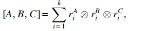
Example 1. Suppose A is a $20 \times 20 \times 20 \times 20 \times 20 \times 20$ 6-way tensor, let $I = {1, 3}$ , $J = {4}$ , and $K = {2, 5, 6}$ . Then $F l a t_{I | J | K} (A)$ is a $2 0^{2} \times 20 \times 2 0^{3}$ tensor with, for example, ${(F l a t_{I | J | K} (A))}_{(10, 12), (8), (15, 16, 18)} = A (10, 15, 12, 8, 16, 18) .$

Kruskal's theorem requires the notion of a 3-way tensor obtained as sum of “outer products” of the rows of 3 matrices.

Definition 3.4. Let A be a $k \times n_{A}$ matrix with $i^{t h}$ row $r_{i}^{A} = (r_{i}^{A} (1), \dots, r_{i}^{A} (n_{A}))$ , and similarly for matrices B and C of size $k \times n_{B}$ and $k \times n_{C}$ , respectively. Then $[A, B, C]$ denotes the 3-way $n_{A} \times n_{B} \times n_{C}$ tensor

where the tensor products in the summands are formatted to preserve an index for each matrix. For instance, , where T denotes the transpose.

To illustrate, suppose that $A, B, C$ are $2 \times 2$ , $2 \times 3$ , and $2 \times 4$ matrices respectively, $A = (\begin{matrix} 1 & 2 \\ 3 & 4 \end{matrix}), B = (\begin{matrix} 1 & 2 & 3 \\ 4 & 5 & 6 \end{matrix}), C = (\begin{matrix} 1 & 2 & 3 & 4 \\ 5 & 6 & 7 & 8 \end{matrix}) .$

Then $P = [A, B, C]$ is the $2 \times 3 \times 4$ tensor with slices with respect to the C index given by $\begin{matrix} P (\cdot, \cdot, 1) = (\begin{matrix} 61 & 77 & 93 \\ 82 & 104 & 126 \end{matrix}), P (\cdot, \cdot, 2) = (\begin{matrix} 74 & 94 & 114 \\ 100 & 128 & 156 \end{matrix}), \\ P (\cdot, \cdot, 3) = (\begin{matrix} 87 & 111 & 135 \\ 118 & 152 & 186 \end{matrix}), P (\cdot, \cdot, 4) = (\begin{matrix} 100 & 128 & 156 \\ 136 & 176 & 216 \end{matrix}) . \end{matrix}$

As a simple extension of Definition 3.4 for use with phylogenetic models, we write

where $π = (π_{1}, π_{2}, \dots, π_{k}) .$

Before stating Kruskal's Theorem, we need the following.

Definition 3.5. Let A be a matrix. The Kruskal (row) rank of a matrix A is the largest number k such that every set of k rows of A is independent.

For example, letting V denote the set of all $3 \times 3$ matrices, a set of dimension 9, consider matrices of the form $(\begin{matrix} a & b & c \\ a & b & c \\ d & e & f \end{matrix}),$ (1)

where $(a, b, c), (d, e, f)$ are independent. These matrices have rank 2 but Kruskal rank 1, and form a subset of lower dimension inside the nine-dimensional space V.

It is clear that Kruskal rank is less than or equal to matrix rank, but when a matrix has full row rank, the two notions coincide. In subsequent sections, we exploit this observation by creating matrices with full row rank and therefore full Kruskal rank.

Kruskal's theorem can be viewed as a generic identifiability theorem for 3-way arrays, showing that triple products satisfying a particular rank condition are decomposable in essentially a unique way.

Theorem 3.6. (Kruskal, 1977). Let $A, B, C$ be $l \times n_{A}$ , $l \times n_{B}$ , and $l \times n_{C}$ matrices with Kruskal rank $p, q, r$ , respectively. If

p + q + r \geq 2 l + 2,

(2)

then $A, B, C$ are uniquely determined by $[A, B, C]$ , up to simultaneous permutation and scaling of their rows. More precisely, if $[A, B, C] = [A', B', C']$ , then there exist invertible diagonal matrices $D_{1}, D_{2}$ and a permutation matrix P such that $A' = P D_{1} A, B' = P D_{2} B, C' = P D_{1}^{- 1} D_{2}^{- 1} C .$

By way of contrast, note that for two compatible matrices A, B, the natural analogue of the bracket product is the matrix product $[A, B] = A^{T} B$ . However, from $[A, B]$ , A and B cannot be determined uniquely, since there are many matrix products that give the same result. For instance, for any orthogonal matrix Q. Kruskal's theorem thus states a significant difference between matrices and 3-way tensors.

3.2. Generic points in parameter space

Algebraic geometry provides a convenient tool for understanding exceptional sets, such as those that fail to satisfy the rank conditions necessary to apply Kruskal's Theorem. We briefly give the needed definitions.

Definition 3.7. Let S be a finite set of polynomials in $ℂ [x_{1}, \dots, x_{n}]$ . The common zero set in $ℂ^{n}$ of the polynomials in S is the algebraic variety $V (S)$ . A subset of a variety that is itself a variety is called a subvariety. For any algebraic variety $V (S) \subseteq ℂ^{n}$ , the ideal $I (V (S))$ is the set of all polynomials $f \in ℂ [x_{1}, \dots, x_{n}]$ such that $f (v) = 0$ for all $v \in V (S)$ .

The main result of this work is that PM model parameters are identifiable except for “rare” choices. This is expressed using the following terminology.

Definition 3.8. A property is generic on a full-dimensional subset W of $ℛ^{n}$ or $ℂ^{n}$ if it holds at all points of W except possibly for those points in some subset $U \subset W$ of measure 0. If V is an algebraic variety in $ℂ^{n}$ , we say a property is generic on V if it holds at all points except those in a proper subvariety of V.

This notion of “generic” on a variety is stricter than that sometimes used in algebraic geometry (a property that holds on a countable intersection of Zariski dense open sets), but is simpler for our purposes. Also, since proper subvarieties of V are of measure 0, our two uses of the word “generic” in the definition are consistent.

Example 2. The set of $3 \times 3$ matrices, viewed as $ℂ^{9}$ , forms a variety $V (S)$ with $S = {0}$ . The property of having rank, or equivalently Kruskal rank 3, is generic on V, since matrices of rank at most 2, including those of the form (1), lie on a subvariety defined by the vanishing of a single polynomial, the $3 \times 3$ determinant. This exceptional set is of dimension 8.

A fundamental tool for drawing conclusions that model parameters are generically identifiable is the following variant of a proposition in Rhodes and Sullivant (2012), which we use repeatedly.

Proposition 3.9. Let $Φ : U \to ℂ^{n}$ be a complex analytic map with U an open subset of $ℂ^{ℓ}$ . Let V be a variety in $ℂ^{n}$ . Suppose $f \in I (V)$ , and that there exists a point $p_{1} = Φ (u_{1})$ with $f (p_{1}) \neq 0$ . Then for generic points $u \in U$ or $u \in U \cap ℛ^{n}$ , the point $Φ (u)$ lies off the variety V.

Proof. This follows from basic properties of complex analytic functions of many variables (see, for instance, the text by Range, 1986). The function $f \circ Φ$ is analytic, and not identically zero. Its zero set is therefore of measure zero, so for generic $u \in U$ , $Φ (u)$ lies off $V (f) \supseteq V$ . The real points in the zero set must similarly have measure zero.

3.3. Rank propositions

For the proof of our main theorem, the ranks and Kruskal ranks of some special matrices arising in the PM model are needed, and we compile these rank computations here. By giving these algebraic results in advance, the proof of Theorem 5.7 can be presented more cleanly. Note that our arguments depend, in part, on some computations that were performed with the software Pari/GP. As these computations were performed using exact integer arithmetic, they may be taken as valid proofs, up to the usual assumptions of correct programming and no hardware faults.

We begin by defining a particular structured matrix (an instance of the equal input model; Casanellas and Steel, 2017) that can arise from particular parameter choices for the PM model.

Definition 3.10. With $a_{i} \in ℂ$ for $i \in [κ]$ , and $s = a_{1} + \dots + a_{κ}$ , let $M (a_{1}, \dots, a_{κ})$ denote the $κ \times κ$ matrix

M (a_{1}, \dots, a_{κ}) = (\begin{matrix} 1 + a_{1} - s & a_{2} & \dots & a_{κ} \\ a_{1} & 1 + a_{2} - s & \dots & a_{κ} \\ ⋮ & ⋱ & ⋮ \\ a_{1} & a_{2} & \dots & 1 + a_{κ} - s \end{matrix}) .

(3)

We next show that $ℓ$ -th row-tensor power of a matrix M formed from m stacked matrices of the form $M (a_{1}, \dots, a_{20})$ generically has full row rank if m is not too large. Part of the argument is inductive, with $ℓ = 3$ as the base case. While the size of $M^{⨂_{r}^{3}}$ is $20 m \times 2 0^{3}$ , only 1540 of the columns turn out to be distinct, so its rank is bounded by $min (20 m, 1540)$ . Thus only by restricting to $m = 1540 ∕ 20 = 77$ classes can we hope to obtain full row rank.

Note, however, that this upper bound of $m \leq 77$ profiles in the proposition below and the slightly stronger restriction to $m < 74$ profiles in our main result Theorem 5.7 are tied to our focus on $κ = 20$ for amino acid models. Even for $κ = 20,$ the restriction to $m < 74$ of the main result is unlikely to be tight, as it is, in part, an artifact of our specific arguments. If PM models with larger m become of interest for data analysis, then our general techniques are likely to extend to their analysis.

Proposition 3.11. For $κ = 20$ and $m \leq 77$ , let M be an $m κ \times κ$ matrix formed by stacking $m \geq 1$ choices of matrices of the form $M (a_{1}, \dots, a_{κ})$ . Then $M^{⨂_{r}^{ℓ}}$ has full row rank for generic choices of the a_i when $ℓ \geq 3$ .

Proof. We begin with the special case of $ℓ = 3$ . An exact Pari/GP calculation shows that for $m = 77$ by picking distinct random integers for $a_{1}, \dots, a_{κ}$ , the $1540 \times 8000$ -matrix $M^{⨂_{r}^{3}}$ has full row rank. By removing some of the blocks from this example if $m < 77$ , we obtain a point p₁ for which $M^{⨂_{r}^{3}}$ has full row rank for smaller m as well.

To show that full row rank is a generic condition when $ℓ = 3$ , fix $m \leq 77$ , and observe that the map from the space $ℂ^{m κ}$ of the a_i to {M} is analytic. Since $p_{1} = M$ gives $M^{⨂_{r}^{3}}$ full row rank, there is some $m κ \times m κ$ minor f of $M^{⨂_{r}^{3}}$ , which when viewed as a polynomial in the entries of M has $f (p_{1}) \neq 0$ . Taking $V = V (f)$ , then Proposition 3.9 shows that generic choices of the a_i give $f (M) \neq 0$ so $M^{⨂_{r}^{3}}$ has rank $m κ$ .

Now consider $ℓ > 3$ . Then $M^{⨂_{r}^{ℓ}} = M^{⨂_{r}^{3}} ⨂_{r} M^{⨂_{r}^{ℓ - 3}}$ , where $M^{⨂_{r}^{3}} = (μ_{i j})$ is a $m κ \times κ^{3}$ matrix and $M^{⨂_{r}^{ℓ - 3}} = (α_{k l})$ is a $m κ \times κ^{ℓ - 3}$ matrix. Since $M^{⨂_{r}^{3}}$ has full row rank $m κ$ for generic M, its rows are independent. However, with $v = m κ$ , $M^{⨂_{r}^{3}} ⨂_{r} M^{⨂_{r}^{ℓ - 3}} = (\begin{matrix} μ_{11} α_{11} & μ_{12} α_{11} & \dots & μ_{1 κ^{3}} α_{11} & \dots \dots \\ μ_{21} α_{21} & μ_{22} α_{21} & \dots & μ_{2 κ^{3}} α_{21} & \dots \dots \\ ⋮ & ⋱ & ⋮ \\ μ_{v 1} α_{v 1} & μ_{v 2} α_{v 1} & \dots & μ_{v κ^{3}} α_{v 1} & \dots \dots \end{matrix}),$

so it is enough to know that the entries of some single column of $M^{⨂_{r}^{ℓ - 3}}$ are nonzero and that $M^{⨂_{r}^{3}}$ has independent rows to ensure $M^{⨂_{r}^{ℓ}}$ has independent rows. However, this is true for generic choices of parameters for M. □

The next proposition gives a lower bound on Kruskal row rank, valid for all $M^{⨂_{r}^{ℓ}}$ .

Proposition 3.12. For $κ \geq 2$ , let M be an $m κ \times κ$ matrix formed by stacking $m \geq 1$ choices of matrices of the form $M (a_{1}, \dots, a_{κ})$ . For $ℓ \geq 1$ , $M^{⨂_{r}^{ℓ}}$ has Kruskal row rank greater than or equal to 2 for generic choices of the a_i.

Proof. Consider first the case that $ℓ = 1$ . The matrices of the form M with Kruskal rank at most 1 form a subvariety V of all such M. By Proposition 3.9, it is enough to find a single matrix M not in V to see that generically such matrices have Kruskal rank at least two. Choose $m κ$ distinct positive small numbers as the free entries $a_{1}, \dots, a_{κ}$ in each block of M, so that the diagonal entries are the largest in the block. Then no two rows within any block $M (a_{1}, \dots, a_{κ})$ are multiples of each other, and no two rows of different blocks are multiples either, since the a_i's are distinct. Thus M has Kruskal rank greater than or equal to two.

The case when $ℓ > 1$ follows by an argument similar to that at the end of the proof of Proposition 3.11.

The final propositions in this section involve generic ranks of stacked matrices formed by taking certain tensor products of matrices of the form above.

Proposition 3.13. Let M be an $m κ^{2} \times κ^{3}$ matrix formed by stacking m choices of matrices of the form . Then for $κ = 20$ and $m < 77$ , the matrix M has rank greater than $m κ$ for generic choices of the a_i.

Proof. A Pari/GP calculation shows that for some choices of random integers a_i, M has

(1)

full row rank $400 > m κ = 20$ , when $m = 1$ ;

(2)

full row rank $800 > m κ = 40$ , when $m = 2$ ;

(3)

rank $1180 > m κ = 60$ , when $m = 3$ ; and

(4)

rank $1540 > m κ = 80$ , when $m = 4$ .

Furthermore, by (4), for $m \geq 5$ , there exists a matrix M with rank at least $1540 = 20 \times 77$ for some choice of a_i’s, since we may repeat some blocks. Using Proposition 3.9, the stated rank condition on M is thus generic for all $m < 77$ .

Proposition 3.14. Let $M_{1} = M$ be as in Proposition 3.13, and M₂ be the rearrangement of M₁ formed by stacking m matrices with the same choices of the a_i. Let L be an $m κ^{2} \times m κ^{2}$ diagonal matrix with positive entries. Then for $κ = 20$ and $m < 74$ , $M_{2}^{T} L M_{1}$ has rank greater than $m κ$ for generic choices of the a_i.

Proof. Sylvester's rank inequality gives $r a n k (M_{2}^{T} L M_{1}) \geq r a n k (M_{2}^{T}) + r a n k (L M_{1}) - m κ^{2} .$

Since M₁ and M₂ differ only by row and column permutations, they have the same rank. Moreover, $r a n k (L M_{1}) = r a n k (M_{1})$ since L is a diagonal matrix with positive entries. Then, by Proposition 3.13, there is a choice of a_i's so that $M_{2}^{T} L M_{1}$ has rank at least

(1)

$400 + 400 - 400 = 400 > m κ = 20$ , when $m = 1$ ;

(2)

$800 + 800 - 800 = 800 > m κ = 40$ , when $m = 2$ ;

(3)

$1180 + 1180 - 1200 = 1160 > m κ = 60$ , when $m = 3$ ; and

(4)

$1540 + 1540 - 1600 = 1480 > m κ = 80$ , when $m = 4$ .

The rank computation for $m = 4$ shows additionally that there exist choices of a_i giving $r a n k (M_{2}^{T} L M_{1}) = 1480$ for larger m, since blocks can be repeated. However, $1480 = 20 \times 74$ and so by Proposition 3.9, generically the rank must be greater than $m κ$ for all $m < 74$ .

4. Algebraic Aspects Of The Pm Model

Next we relate the algebraic definitions made in the previous section to phylogenetic models and the PM model in particular. We begin by describing how a row tensor product of Markov matrices relates to parameters on a star tree.

Definition 4.1. Let A be a set of taxa on a star tree rooted at its internal node, with pendant edges $e_{1}, \dots, e_{| A |}$ and associated Markov matrices $M^{e_{i}}$ . Then

M_{A} = M^{e_{1}} ⨂_{r} \dots ⨂_{r} M^{e_{| A |}} .

(4)

For an m-class PM model on a star tree, the matrix M_A is of size $m κ \times κ^{| A |}$ . Its entries are conditional probabilities of observing different $| A |$ -tuples of states at the taxa in set A, given the state at the root.

Given a tree T on taxa X, tripartitions and splits of X can be associated with the topological structure of T. For instance, the tree of Figure 1 displays a tripartition $A | B | C$ with $A = {a, b, c}, B = {d, f}, C = {g, h}$ . Formally, a tripartition $A | B | C$ is displayed on a tree if there is some vertex v of T whose deletion results in three subtrees with $A, B, C$ labeling their leaves. Similarly, if $A' = {a, b, c}$ and $B' = {d, f, g, h}$ , then $X = A' ⨆ B'$ , and T displays the split $A' | B'$ of X, since there is an edge e whose deletion results in two subtrees with leaves labeled by $A'$ and $B'$ .

FIG. 1.

A tree displaying the tripartition $A | B | C$ and the split $A | B \cup C$ , where $A = {a, b, c}, B = {d, f}, C = {g, h}$ .

When a tree T displays a tripartition of a set of taxa, then the flattening of a joint distribution corresponding to that tripartition can be expressed using the 3-way matrix product of certain matrices built from model parameters.

Lemma 4.2. Suppose T is a tree on a set of taxa X rooted at an internal vertex v and that T displays the tripartition $A | B | C$ associated with v. Let P be a probability distribution for a Markov model $ℳ$ on T with $ℓ$ states at the internal nodes. Then there exist matrices ${\bar{M}}_{A}$ , ${\bar{M}}_{B}$ , ${\bar{M}}_{C}$ constructed from model parameters for $ℳ$ , each with $ℓ$ rows, such that

F l a t_{A | B | C} (P) = [{\bar{M}}_{A}, {\bar{M}}_{B}, {\bar{M}}_{C}] .

Proof. From the parameters on T we may define Markov matrices $M_{A}, M_{B}, M_{C}$ whose entries are conditional probabilities of states at the leaves in each set $A, B, C$ , given the state at v. Let π be the state distribution at v. Then $F l a t_{A | B | C} (P) = [π; M_{A}, M_{B}, M_{C}] = [{\bar{M}}_{A}, {\bar{M}}_{B}, {\bar{M}}_{C}],$

where ${\bar{M}}_{A} = d i a g$ (π) $M_{A}$ , ${\bar{M}}_{B} = M_{B}$ , and ${\bar{M}}_{C} = M_{C}$ .

For establishing generic properties of the PM model, we often consider the particular choice of the exchangeabilities given by the matrix $R = \infty$ whose entries are all 1. This is, in essence, the CAT-F81 model (Lartillot and Philippe, 2004; Le et al., 2008), with the number of profiles some fixed m. For this R, a Markov matrix has the form given in Equation (3) of Definition 3.10.

Lemma 4.3. Consider the PM model $P M (T, κ, m)$ with $R = \infty$ , and let e be a branch of T of length 1. Then for a single-class $c \in [m]$ with profile π and rate $r \geq 0$ , the Markov matrix $M_{c}^{e} = exp (r Q_{c})$ for e is of the form $M (a_{1}, \dots, a_{κ})$ of Definition 3.10, with $a_{i} = π_{i} (1 - e^{- r}) \geq 0$ and $s = \sum_{i = 1}^{κ} a_{i}$ satisfying $0 \leq s < 1$ .

Conversely, any $κ \times κ$ Markov matrix of the form $M = M (a_{1}, \dots, a_{κ})$ with $a_{j} \geq 0$ and $0 \leq s < 1$ comes from a choice of parameters for one class of the PM model with $R = \infty$ on an edge of length 1.

Provided $s \neq 0$ (equivalently $r \neq 0$ ), this correspondence is one-to-one.

Proof. The first statement follows by direct computation: With $e_{j}$ the standard basis vectors, $Q_{c} = R d i a g$ (π) $- I$ has right eigenvectors $- π_{j} e_{1} + π_{1} e_{j}$ with eigenvalues $- 1$ for $2 \leq j \leq κ$ , and eigenvector $\sum_{j = 1}^{κ} e_{j}$ with eigenvalue 0.

For the converse, since $0 \leq s < 1$ , there is a unique $r \geq 0$ such that $s = 1 - e^{- r}$ . If $s > 0$ , let $π_{j} = a_{j} ∕ s$ for $j = 1, \dots, κ$ , and π $= (π_{j})$ . Then $\sum_{j = 1}^{κ} π_{j} = 1$ , and $a_{j} = π_{j} (1 - e^{- r})$ . With these choices, $Q = R d i a g$ (π) $- I$ and $M = exp (r Q)$ . If $s = 0$ , then all the a_j are zero, and M is the identity matrix. Take $r = 0$ and π arbitrary. Then $M = exp (0 Q) .$

5. Identifiability of Parameters For the Pm Model

With preliminaries completed, we now turn to establishing our main result, on generic parameter identifiability for the PM model. The first step is to understand that the ranks of matrix flattenings of a model distribution are affected by whether the associated split is, or is not, displayed on the tree T.

Proposition 5.1. Let T be an n-taxon tree on X and P a distribution from the model PM = PM $(T, κ, m)$ with $κ = 20$ and $m < 74$ . Suppose that $A | B$ is a split of X with $| A |, | B | \geq 3$ .

(1)

If $A | B$ is displayed on T, then $F l a t_{A | B} (P)$ has rank at most $m κ$ ;

(2)

If $A | B$ is not displayed on T, then $F l a t_{A | B} (P)$ generically has rank greater than $m κ$ .

Before beginning the proof, we present a simplified example to illustrate how the matrix rank of flattenings of joint distributions from Markov models on trees carries information about the absence/presence of internal edges on T.

Example 3. Consider a single-class 2-state Markov model on the 4-taxon tree shown in Figure 2. A special case of this model is $P M (T, 2, 1)$ . The joint distribution of states at the leave of T is the $2 \times 2 \times 2 \times 2$ array P, with entries $p_{i j k l}$ indexed by leaves in the order $a, b, c, d$ .

FIG. 2.

A 4-taxon tree with split ${a, b} | {c, d}$ .

With $A = {a, b}$ and $B = {c, d}$ , the rows and columns of $F l a t_{A | B} (P)$ are indexed by elements of $[2] \times [2]$ . For example, the $((1, 2), (1, 1))$ entry is $p_{1211}$ . In contrast, if $A' = {a, c}$ and $B' = {b, d}$ , the flattening $F l a t_{A' | B'} (P)$ has $((1, 2), (1, 1))$ -entry is $p_{1121}$ .

Now suppose that the terminal edges of T have length 0, so that the states at a and b must agree, as must those at c and d, since no substitutions occur on terminal edges. Then the matrix $F l a t_{A | B} (P)$ arises from the joint distribution of states at the internal nodes v₁ and v₂, and its only nonzero entries are $p_{i i j j}$ . Thus the matrix flattening for the split $A | B$ displayed by T has form $F l a t_{A | B} (P) = \begin{matrix} (1, 1) \\ (1, 2) \\ (2, 1) \\ (2, 2) \end{matrix} (\begin{matrix} (1, 1) & (1, 2) & (2, 1) & (2, 2) \\ p_{1111} & 0 & 0 & p_{1122} \\ 0 & 0 & 0 & 0 \\ 0 & 0 & 0 & 0 \\ p_{2211} & 0 & 0 & p_{2222} \end{matrix}),$

with rank at most $2 = m κ$ .

In contrast, the flattening for the split $A' | B'$ not displayed on T has form $F l a t_{A' | B'} (P) = \begin{matrix} (1, 1) \\ (1, 2) \\ (2, 1) \\ (2, 2) \end{matrix} (\begin{matrix} (1, 1) & (1, 2) & (2, 1) & (2, 2) \\ p_{1111} & 0 & 0 & 0 \\ 0 & p_{1122} & 0 & 0 \\ 0 & 0 & p_{2211} & 0 \\ 0 & 0 & 0 & p_{2222} \end{matrix}),$

which generically has rank

If the terminal edges of T are of positive length, then the resulting joint distribution P can be obtained by a simple and generically rank-preserving linear action on the rows and columns of the flattenings above, as described in Allman and Rhodes (2006). Thus, flattenings respecting the topology of T generically have rank $m κ$ , while those that do not generically have larger rank.

Proof of Proposition 5.1.

Claim (1) follows from Lemma 4.1 of Rhodes and Sullivant (2012), since the PM model is a submodel of a mixture of m general Markov models on a single tree.

For claim (2), suppose now $A | B$ is not displayed on T. Let V be the variety of matrices of size $κ^{| A |} \times κ^{| B |}$ with rank at most $m κ$ , defined by the set of all $(m κ + 1) \times (m κ + 1)$ minors. By Proposition 3.9, it suffices to find a single choice of $P M (T, κ, m)$ parameters that produces a point off V, as the parameterization extends to a complex analytic function.

Since T does not display $A | B$ , by Theorem 3.8.6 of Semple and Steel (2003), there is an edge $e = (v_{1}, v_{2})$ of T with associated split $C | D$ such that $A' = A \cap C$ , $A'' = A \cap D$ , $B' = B \cap C$ , and $B'' = B \cap D$ are all nonempty. To find the needed choice of parameters, fix all internal edges of T except e to have length $0,$ so the Markov matrices on these edges are I, and fix the edge lengths of all terminal edges and e to be 1 (Fig. 3). Take $R = \infty$ and mixing weights $w_{i} = 1 ∕ m$ to be uniform. Values for the parameters $π_{i}, r_{i}$ are specified later in the argument. For this choice of parameters, T is formed by joining two star trees at the ends of e.

Taking $r = v_{1}$ to be the root of T, let $K = d i a g (Π) M^{e}$ be the $m κ \times m κ$ block diagonal matrix, which is the joint distribution of classes and states at v₁ and v₂. The probabilities of observing states i , j , k , l at leaves in $A'$ , $B'$ , $A''$ , $B''$ , respectively, $P (i, j, k, l)$ , are the entries of a $κ^{| A' |} \times κ^{| B' |} \times κ^{| A'' |} \times κ^{| B'' |}$ tensor.

Define an $m κ \times m κ \times m κ \times m κ$ tensor $\bar{Q}$ , $\bar{Q} (i, j, k, l) = \{\begin{matrix} K (i, k) & i = j, k = l, \\ 0 & o t h e r w i s e . \end{matrix}$

The tensor $\bar{Q}$ is the joint distribution of states at the leaves of the tree T of Figure 3 when terminal edges have length zero and $A', B', A'', B''$ are single taxa. Indeed, since $A | B$ is not displayed on T, the matrix $\hat{Q} = F l a t_{A | B} (\bar{Q})$ is with entries $\hat{Q} ((i, j), (k, l)) = \bar{Q} (i, k, j, l) .$

Since K is block diagonal, $\hat{Q}$ has at most $m κ^{2}$ nonzero entries, all appearing on the diagonal, and $\hat{Q}$ is generically of rank $m κ^{2}$ .

To see that in the general case $F l a t_{A | B} (P)$ has a similar structure, let $N_{A} = M_{A'} ⨂ M_{A''}$ and $N_{B} = M_{B'} ⨂ M_{B''}$ where $M_{A'}, M_{A''}, M_{B'}, M_{B''}$ are given as in Equation (4) of Definition 4.1. Then $F l a t_{A | B} (P) = N_{A}^{T} \hat{Q} N_{B} .$ (5)

We now establish that claim (2) holds when $| A | = | B | = 3$ , so the tree is one of those shown in Figure 4. Suppose first that $| A' | = | B' | = 2$ and $| A'' | = | B'' | = 1$ , as shown for tree (a) of the figure. In this case $N_{A} = N_{B}$ . Since $\hat{Q}$ is diagonal with at most $m κ^{2}$ nonzero entries due to the block structure of K, in Equation (5) we can replace $\hat{Q}$ by a diagonal $m κ^{2} \times m κ^{2}$ matrix Q by eliminating zero rows and columns. To do this, we must also replace $N_{A} = N_{B}$ with an $m κ^{2} \times κ^{3}$ matrix N formed by taking tensor products of the individual class components of $M_{A'} = M^{⨂_{r}^{2}}$ and $M_{A^{''}} = M$ and then restacking. To be concrete, for class c, the Markov matrix for a terminal edge is $M^{c} = M (a_{1}^{c}, \dots, a_{κ}^{c})$ by Lemma 4.3, and N is formed by stacking m matrices .

Since Q is diagonal with generically positive entries, using Equation (5) we have that $F l a t_{A | B} (P) = (N^{T} Q^{1 ∕ 2}) (Q^{1 ∕ 2} N) = Λ^{T} Λ,$

where $Λ = Q^{1 ∕ 2} N$ . By the singular value decomposition, it follows that $r a n k (Λ^{T} Λ) = r a n k (Λ) = r a n k (N) .$

The Pari/GP calculation presented in Proposition 3.13, together with Proposition 3.9, shows $r a n k (N) > m κ$ generically, and thus, for generic $π_{i}$ and r_i it follows that $r a n k (F l a t_{A | B} (P)) > m κ$ .

Now continuing with $| A | = | B | = 3$ suppose that $| A' | = | B'' | = 2$ and $| A'' | = | B' | = 1$ , as shown in Figure 4b. The previous argument fails for this tree because now $N_{A} \neq N_{B}$ , as the tensor products defining these matrices are taken in different orders. However, a more complicated Pari/GP calculation, presented as Proposition 3.14, shows that $F l a t_{A | B} (P)$ generically has rank greater than $m κ$ in this case.

Finally, for the general case of $| A |, | B | \geq 3$ , take $Â$ to be a 3-element subset of A with at least one element from $A'$ and one from $A''$ , and similarly take $\hat{B}$ to be a 3-element subset of B with at least one element from $B'$ and from $B''$ . Let $\hat{P}$ be the probability distribution for the taxa $Â \cup \hat{B}$ . Since the row indices of $F l a t_{A | B} (P)$ depend on the states at the taxa in A and the column indices depend on the states at the taxa in B, marginalizing over all possible states for the taxa in A, which are not in $Â$ , and similarly for B, gives the matrix $F l a t_{Â | \hat{B}} (\hat{P})$ . There exist matrices, $J_{1}, J_{2}$ , that perform this marginalization on $F l a t_{A | B} (P)$ , $J_{1} F l a t_{A | B} (P) J_{2} = F l a t_{Â | \hat{B}} (\hat{P}) .$

Since $F l a t_{Â | \hat{B}} (\hat{P})$ generically has rank greater than $m κ$ and $F l a t_{A | B} (P)$ has rank greater than or equal to $F l a t_{Â | \hat{B}} (\hat{P})$ by this equation, it follows that $F l a t_{A | B} (P)$ generically has rank greater than $m κ$ .

FIG. 3.

A tree T that does not display the split $A | B$ with $A = A' \cup A''$ , $B = B' \cup B''$ , but displays the split $C | D$ with $C = A' \cup B'$ and $D = A'' \cup B''$ .

FIG. 4.

Trees with (a) $| A' | = | B' | = 2$ and $| A'' | = | B'' | = 1$ , and (b) $| A' | = | B'' | = 2$ and $| A'' | = | B' | = 1$ .

As a consequence of Proposition 5.1, from a distribution P computed from generic PM model parameters we can identify every edge in the tree for which there are at least three taxa on either side, by computing ranks of flattenings of P. In the following, we see that Proposition 5.1 also helps to identify at least one tripartition on the tree.

Proposition 5.2. Let T be an n-taxon tree on X with $n \geq 9$ , and P a joint distribution from generic parameters for the model $P M (T, κ, m)$ with $κ = 20$ and $m < 74$ . Then there is at least one tripartition $A | B | C$ displayed on T, with $| A |, | B | \geq 3$ , which can be identified from P.

Proof. By Lemma $4.8$ of Rhodes and Sullivant (2012), every unrooted binary tree T with $n \geq 3$ has an internal vertex v, which induces a tripartition $A | B | C$ such that two of the three components contain at least $⌈ n ∕ 4 ⌉$ leaves of T.

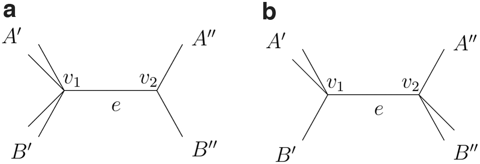
The two edges incident to v that corresponds to subsets of X with at least $⌈ n ∕ 4 ⌉$ leaves are generically identifiable by Proposition 5.1, since for $n \geq 9$ , $⌈ n ∕ 4 ⌉ \geq 3$ . If the third edge incident to v has 3 or more taxa in its component, it also can be identified. Thus, it remains to establish that the third edge incident to v can be identified when the number of taxa in its component is 1 or 2. Examples of such trees are illustrated for $n = 9$ in Figure 5a,b.

If the third component has only one leaf, as in Figure 5a, the two bipartitions $A \cup {c} | B$ and $A | B \cup {c}$ are identifiable by Proposition 5.1. Together this implies that the tripartition induced by v is $A | B | {c}$ . If the third component has two leaves as in Figure 5b, the two splits $A \cup {c_{1}, c_{2}} | B$ and $A | B \cup {c_{1}, c_{2}}$ are identifiable, but $A \cup {c_{1}} | B \cup {c_{2}}$ and $A \cup {c_{2}} | B \cup {c_{1}}$ are not displayed on T, and that can be detected by Proposition 5.1. This implies that the tripartition $A | B | {c_{1}, c_{2}}$ is on the tree.

FIG. 5.

Examples of 9-taxon trees with internal vertex v inducing $A | B | C$ with $| A |, | B | \geq 3$ and $| C | = 1$ or 2.

With a tripartition on the tree identifiable by the preceding proposition, we prepare to apply Kruskal's Theorem. Letting P be a joint distribution from $P M (T, κ, m)$ , pick an internal vertex v of T inducing such a tripartition $A | B | C$ . Then by Lemma 4.2 $F l a t_{A | B | C} (P) = [π; M_{A}, M_{B}, M_{C}] = [{\bar{M}}_{A}, M_{B}, M_{C}],$

where ${\bar{M}}_{A} = d i a g (Π) M_{A}$ . Provided the Kruskal ranks of the matrices ${\bar{M}}_{A}, M_{B}, M_{C}$ are large enough, at least generically, Kruskal's theorem can be applied. The next three lemmas establish this.

Lemma 5.3. Consider the model $P M (T, 20, m)$ with $m \leq 77$ . If $ℓ \geq 3$ , then the $ℓ^{t h}$ row tensor power of the $m κ \times κ$ Markov matrix associated with a terminal edge of T has full row rank for generic parameters.

Proof. Using Proposition 3.9, it is enough to show there is a single choice of parameters for which the tensor power has full row rank. Let R = 1, and take the terminal branch lengths to be 1. Then by Lemma 4.3, the Markov matrix M_e on a terminal edge has the form of stacked matrices of the form $M (a_{1}, \dots, a_{κ})$ . By the Pari/GP calculation of Proposition 3.11, for generic choices of the other parameters, $M_{e}^{⨂_{r}^{ℓ}}$ , $ℓ \geq 3$ , has full row rank.

Using Proposition 3.12 in a similar argument we obtain the following.

Lemma 5.4. Consider the model $P M (T, κ, m)$ with $κ \geq 2$ and $m \geq 1$ . Then for $ℓ \geq 1$ , the $ℓ^{t h}$ row tensor power of the $m κ \times κ$ Markov matrix associated with a terminal edge of T generically has Kruskal rank at least 2.

Lemma 5.5. For a distribution from the model $P M (T, κ, m)$ with $κ = 20$ and $m \leq 77$ , let ${\bar{M}}_{A}, M_{B}, M_{C}$ be the matrices described above. If $| A |, | B | \geq 3$ , and $| C | \geq 1$ , then generically ${\bar{M}}_{A}$ , M_B have full Kruskal rank and M_C has Kruskal rank at least 2.

Proof. Using Proposition 3.9, we need only show there is a single choice of parameters for which these rank claims hold. Set all internal branch lengths 0 and all terminal branch lengths 1, so that T is a star tree rooted at the central node v. Then by Lemma 5.3, since $| A |, | B | \geq 3$ for generic choices of the profiles π_i, the matrices M_A (and therefore ${\bar{M}}_{A}$ ) and M_B have full row rank and therefore full Kruskal rank. Also by Lemma 5.4, M_C has Kruskal rank at least 2.

We add the last ingredient before the main result.

Proposition 5.6. Suppose T is a tree on X that displays a known tripartition $A | B | C$ corresponding to vertex r with $| A |, | B | \geq 3$ , $| C | \geq 1$ . If $κ = 20$ and $m \leq 77$ then both T and the numerical parameters of the PM $(T, κ, m)$ model are generically identifiable, up to arbitrary rescaling of the tree and the exchangeability matrix R.

Proof. Using the notation and result of Lemma 5.5, if a distribution P comes from generic parameters of $P M (T, κ, m)$ , then $F l a t_{A | B | C} (P) = [{\bar{M}}_{A}, M_{B}, M_{C}],$

where ${\bar{M}}_{A}, M_{B}$ have full Kruskal rank and M_C has Kruskal rank at least 2. Thus Equation (2) of Theorem 3.6 is satisfied with $l = m κ$ , and ${\bar{M}}_{A}, M_{B}, M_{C}$ are determined uniquely up to simultaneous permutation and scaling of the rows.

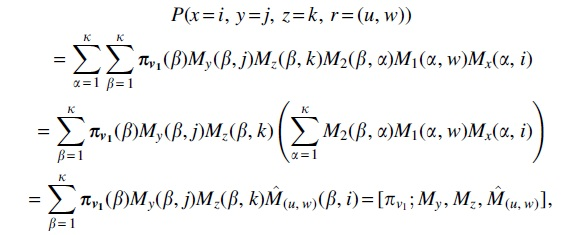
Also, by factoring out row sums from the matrices, we can generically identify the root distribution vector $Π$ at the node r and $M_{A}, M_{B}, M_{C}$ up to simultaneous permutation of the entries of $Π$ and the rows of the matrices. Considering any entry of $Π$ , and supposing that this corresponds to an unknown class $u \in [m]$ and state $w \in [κ]$ , then the same rows of $M_{A}, M_{B}, M_{C}$ correspond to the same class u and state w. Since Kruskal's theorem yields identifiability only up to permutation, we must determine which of the $m κ$ rows of $M_{A}, M_{B}, M_{C}$ correspond to the same fixed class u.

Consider first the special case that $| A | = 3$ where $A = {a, b, c}$ . Then T, which is generically binary, has a subtree rooted at r, with leaves $A = {x, y, z}$ as shown in Figure 6, although we do not know which two taxa from $a, b, c$ form the cherry ${y, z} .$

The Markov matrix M_A is of size $m κ \times κ^{3}$ . Choose the $ℓ^{t h}$ row of M_A where $ℓ = (u, w)$ for unknown $u, w$ . It is a row vector with $κ^{3}$ entries, but we can reconfigure it as a three-dimensional tensor of size $κ \times κ \times κ$ so its $(i, j, k)$ -entry is $P (a = i, b = j, c = k | r = ℓ)$ . Since the PM model is time reversible, take v₁ as the root of the subtree in Figure 6. Then for unknown $1 \times κ$ vector π $_{v_{1}}$ , and $κ \times κ$ Markov matrices $M_{x}, M_{y}, M_{z}, M_{1}, M_{2}$ for class u on this subtree, the joint distribution of states at $x, y, z, r$ for fixed class u is

where ${\hat{M}}_{(u, w)} = M_{2} d i a g (M_{1} (\cdot, w)) M_{x}$ with $M_{1} (\cdot, w)$ denoting the $w^{t h}$ column of M₁. For fixed u this is simply a rescaling of the conditional distribution $P (x = i, y = j, z = k | r = (u, w))$ given in the $ℓ^{t h}$ row of M_A.

Thus applying Kruskal's theorem to each row of M_A reshaped into such a 3-way tensor, we can decompose $P (x = i, y = j, z = k | r = ℓ)$ for each $ℓ = (u, w)$ into a triple product, as the matrices generically all have rank $κ$ . Note that for each $ℓ = (u, w)$ , Kruskal's theorem gives the matrices $M_{y}, M_{z}, {\hat{M}}_{(u, w)}$ up to ordering of their $κ$ rows. Two of these matrices, $M_{y}, M_{z}$ , will be dependent only on the class u, but not the state w. So considering all $ℓ = (u, w)$ , we can find $κ$ rows of M_A with the same (possibly permuted rows) version of M_y and M_z, corresponding to a single-class u. In this way, we can group the rows of $M_{A}, M_{B}, M_{C}$ with entries of $Π$ by class u. Now taking those rows of $M_{A}, M_{B}, M_{C}$ and entries of $Π$ for one class u and reassembling them in a 3-way product gives a tensor for a single-class GTR model on the full tree T. Both the tree T and numerical parameters are identifiable for this single-class model by Theorem 2.4.

For the general case, suppose $| A |, | B | \geq 3$ . Then by marginalization down to $| A | = 3$ , we can identify the subtrees and parameters for $B, C$ . Then interchanging the roles of A and B identifies the subtree and parameters for A.

FIG. 6.

A subtree of T with leaves $A = {a, b, c} = {x, y, z}$ .

Combining Proposition 5.2 with Proposition 5.6, we have proved the main result.

Theorem 5.7. Let T be a tree with at least 9 taxa. Then under the PM $(T, 20, m)$ model with $m < 74$ , both T and numerical parameters are generically identifiable, up to arbitrary rescaling of the tree and the exchangeability matrix R.

Theorem 5.7 extends to certain tree shapes with fewer than 9 taxa. To apply Proposition 5.6, T must display a tripartition with two of its subsets of size at least 3, so that T must have at least 7 taxa. Such a tripartition will be generically identifiable by the argument given for Proposition 5.2.

Corollary 5.8. For the PM model $P M (T, 20, m)$ with $m < 74$ , parameters are generically identifiable if T has any of the 8-taxon tree shapes (a)-(d) shown in Figure 7, or the 7-taxon caterpillar shape.

FIG. 7.

All binary unrooted tree shapes for 8 taxa. Parameters of the profile mixture model are generically identifiable for trees (a–d). The arguments of this article do not answer the identifiability question for tree (e).

Footnotes

Author Disclosure Statement

No competing financial interests exist.

Funding Information

This research was supported, in part, by the National Institutes of Health Grant R01 GM117590, awarded under the Joint DMS/NIGMS Initiative to Support Research at the Interface of the Biological and Mathematical Sciences.

References

Allman

, Ané

, and Rhodes

2008. Identifiability of a Markovian model of molecular evolution with gamma-distributed rates. Adv. Appl. Probab. 40, 229–249.

Allman

, Holder

, and Rhodes

2010. Estimating trees from filtered data: Identifiability of models for morphological phylogenetics. J. Theor. Biol. 263, 108–119.

Allman

, Long

, and Rhodes

2019. Species tree inference from genomic sequences using the log-det distance. SIAM J. Appl. Algebra Geometry. 3, 1–30.

Allman

, Matias

, and Rhodes

2009. Identifiability of parameters in latent structure models with many observed variables. Ann. Statist. 37, 3099–3132.

Allman

, Petrović

, Rhodes

, et al. 2011. Identifiability of two-tree mixtures for group-based models. IEEE/ACM Trans. Comput. Biol. Bioinform. 8, 710–722.

Allman

, and Rhodes

2006. The identifiability of tree topology for phylogenetic models, including covarion and mixture models. J. Comput. Biol. 13, 1101–1113.

Allman

, and Rhodes

2008. Identifying evolutionary trees and substitution parameters for the general Markov model with invariable sites. Math. Biosci. 211, 18–33.

Allman

, and Rhodes

2009. The identifiability of covarion models in phylogenetics. IEEE/ACM Trans. Comput. Biol. Bioinform. 6, 76–88.

Casanellas

, and Steel

2017. Phylogenetic mixtures and linear invariants for equal input models. J. Math. Biol. 74, 1107–1138.

10.

Chai

, and Housworth

2011. On Rogers's Proof of Identifiability for the GTR + Gamma + I Model. Syst. Biol. 60, 713–718.

11.

Chifman

, and Kubatko

2015. Identifiability of the unrooted species tree topology under the coalescent model with time-reversible substitution processes, site-specific rate variation, and invariable sites. J. Theor. Biol. 374, 35–47.

12.

Hollering

, and Sullivant

2019. Identifiability in phylogenetics using algebraic matroids. arXiv:1909.13754.

13.

Jones

, Taylor

, and Thornton

1992. The rapid generation of mutation data matrices from protein sequences. Comput. Appl. Biosci. 8, 275–282.

14.

Kruskal

1977. Three-way arrays: Rank and uniqueness of trilinear decompositions, with application to arithmetic complexity and statistics. Linear Algebra Appl. 18, 95–138.

15.

Lartillot

, Brinkmann

, and Philippe

2007. Suppression of long-branch attraction artefacts in the animal phylogeny using a site heterogeneous model. BMC Evol. Biol. 7, S4.

16.

Lartillot

, Lepage

, and Blanquart

2009. PhyloBayes 3: A Bayesian software package for phylogenetic reconstruction and molecular dating. Bioinformatics. 25, 2286–2288.

17.

Lartillot

, and Philippe

2004. A Bayesian mixture model for across-site heterogeneities in the amino-acid replacement process. Mol. Bio. Evol. 21, 1095–1109.

18.

Lartillot

, Rodrigue

, Stubbs

, et al. 2013. PhyloBayes MPI: Phylogenetic reconstruction with infinite mixtures of profiles in a parallel environment. Syst. Biol. 62, 611–615.

19.

, Gascuel

, and Lartillot

2008. Empirical profile mixture models for phylogenetic reconstruction. Bioinformatics. 24, 2317–2323.

20.

Long

, and Sullivant

2015. Identifiability of 3-class Jukes-Cantor mixtures. Adv. Appl. Math. 64, 89–110.

21.

Range

1986. Holomorphic Functions and Integral Representations in Several Complex Variables, Vol. 108. Springer-Verlag, New York.

22.

Rannala

2002. Identifiability of parameters in MCMC Bayesian inference of phylogeny. Syst. Biol. 51, 754–760.

23.

Rhodes

, and Sullivant

2012. Identifiability of large phylogenetic mixture models. Bul. Math. Biol. 74, 212–231.

24.

Semple

, and Steel

2003. Phylogenetics, Vol. 24. Oxford University Press, Oxford.

25.

The PARI Group. 2019. PARI/GP version 2.11.2 [Computer software manual]. University of Bordeaux. Available at: http://pari.math.u-bordeaux.fr. Accessed April 15, 2021.

26.

Wang

H.-C.

, Li

, Susko

, et al. 2008. A class frequency mixture model that adjusts for site-specific amino acid frequencies and improves inference of protein phylogeny. BMC Evol. Biol. 8, 1–13.

27.

Wang

H.-C.

, Susko

, and Roger

2014. An amino acid substitution-selection model adjusts residue fitness to improve phylogenetic estimation. Mol. Biol. Evol. 31, 779–792.

28.

Wascher

, and Kubatko

2021. Consistency of SVDQuartets and maximum likelihood for coalescent-based species tree estimation. Syst. Biol. 70, 33–48.

29.

Whelan

, and Goldman

2001. A general empirical model of protein evolution derived from multiple protein families using a maximum-likelihood approach. Mol. Bio. Evol. 18, 691–699.

30.

Yang

1994. Maximum likelihood phylogenetic estimation from DNA sequences with variable rates over sites: Approximate methods. J. Mol. Evol. 39, 306–314.