Polynomial-Time Statistical Estimation of Species Trees Under Gene Duplication and Loss

Abstract

Phylogenomics—the estimation of species trees from multilocus data sets—is a common step in many biological studies. However, this estimation is challenged by the fact that genes can evolve under processes, including incomplete lineage sorting (ILS) and gene duplication and loss (GDL), that make their trees different from the species tree. In this article, we address the challenge of estimating the species tree under GDL. We show that species trees are identifiable under a standard stochastic model for GDL, and that the polynomial-time algorithm ASTRAL-multi, a recent development in the ASTRAL suite of methods, is statistically consistent under this GDL model. We also provide a simulation study evaluating ASTRAL-multi for species tree estimation under GDL.

1. Introduction

Phylogeny estimation is a statistically and computationally complex estimation problem, due to heterogeneity across the genome resulting from processes such as incomplete lineage sorting (ILS), gene duplication and loss (GDL), rearrangements, gene flow, horizontal gene transfer (HGT), and introgression (Maddison, 1997).

Much is known about the problem of estimating species trees in the presence of ILS, as modeled by the multispecies coalescent (MSC) (Kingman, 1982; Takahata, 1989). For example, because the most probable unrooted tree for every four species is the species tree on those species (Allman et al., 2011), the unrooted species tree topology is identifiable under the MSC from its gene tree distribution, and quartet-based species tree estimation methods that operate by combining gene trees [such as BUCKy-pop (Larget et al., 2010) and ASTRAL (Mirarab et al., 2014; Mirarab and Warnow, 2015; Zhang et al., 2018)] are statistically consistent estimators of the unrooted species tree topology (i.e., as the number of sampled genes increases, almost surely the tree returned by these methods will be the true species tree). It is also known that concatenation (whether partitioned or unpartitioned) is not statistically consistent, and can even be positively misleading (i.e., converge to the wrong tree as the number of loci increases) (Roch and Steel, 2015; Roch et al., 2018). In general, establishing whether a method is statistically consistent or not is important for understanding its performance guarantees.

Yet, correspondingly little has been established about species tree estimation in the presence of GDL. For example, although likelihood-based approaches for species tree estimation have been developed [e.g., PHYLDOG (Boussau et al., 2013)], they have not been established to be statistically consistent. Key to understanding the performance of species tree estimation under GDL is whether the species tree topology itself is identifiable from the distribution it defines on the gene trees it generates. However, since gene trees can have multiple copies of each species when gene duplication occurs, this question can be formulated as: “Is the species tree identifiable from the distribution on MUL-trees?” where an MUL-tree is a tree with potentially multiple copies of each species.

In this article, we prove that unrooted species tree topologies are identifiable from the distribution implied on MUL-trees (Section 3) under the simple GDL model of Arvestad et al. (2009). Furthermore, we prove that the polynomial-time method ASTRAL-multi (Rabiee et al., 2019), a recent variant of ASTRAL designed to enable analyses of data sets with multiple individuals per species, is statistically consistent under this model (Section 3). We then present an experimental study evaluating ASTRAL-multi on 16-taxon data sets simulated under the DLCoal model (a unified model of GDL and ILS) (Rasmussen and Kellis, 2012); the results of this study show that when given a sufficiently large number of genes, ASTRAL-multi is competitive with other methods [e.g., DupTree (Bansal et al., 2010), MulRF (Chaudhary et al., 2014), and ASTRID-multi (Vachaspati and Warnow, 2015), the implementation of ASTRID for multiallele data sets] that also estimate species trees from MUL-trees (Section 4). We conclude with remarks about future work and implications for large-scale species tree estimation (Section 5).

Following the publication of the conference version of this work (Legried et al., 2020), identifiability of the species tree was extended by Markin and Eulenstein (2020); Hill et al. (2020) to the DLCoal (Rasmussen and Kellis, 2012), a unified model of GDL and ILS, and sample complexity results were obtained for ASTRAL/ONE under the DLCoal (Hill et al., 2020).

2. Species Tree Estimation from Gene Families

Our input is a collection $T$ of gene trees representing the inferred evolutionary histories of gene families. In the presence of GDL events, such gene trees may be multilabeled trees (MUL-trees), meaning that the same species label may be assigned to several gene copies. Our goal is to reconstruct a species tree T over the corresponding set S of species.

2.1. Astral

We provide theoretical guarantees and empirically validate an approach based on ASTRAL (Mirarab et al., 2014) in its variant for multiple alleles (Rabiee et al., 2019), which we refer to as ASTRAL-multi. Following Du et al. (2019), the input consists of unrooted MUL-trees $T$ from all gene families, where copies of a gene in a species are treated as multiple alleles within the species.

ASTRAL-multi proceeds as follows. Let S be the set of n species and let R be the set of m individuals. The input are the gene trees $T = {t_{i}}_{i = 1}^{k}$ , where t_i is labeled by individuals $R_{i} \subseteq R$ . For any (unrooted) species tree $\tilde{T}$ labeled by S, an extended species tree ${\tilde{T}}_{e x t}$ labeled by R is built by adding to each leaf of $\tilde{T}$ all individuals corresponding to that species as a polytomy. The quartet score of $\tilde{T}$ with respect to $T$ is then

where $1 (T_{1}, T_{2})$ is the indicator that T₁ and T₂ agree and $T_{1}^{J}$ is the restriction of T₁ to individuals $J$ . Run in its exact version (i.e., an unrooted species tree that maximizes the quartet score), ASTRAL-multi is guaranteed to find an optimal solution, but can use exponential time. The default mode, which runs in polynomial time, uses dynamic programming to solve a constrained version of the problem, requiring that the output tree draw its bipartitions from a set $Σ$ of bipartitions that ASTRAL computes on the input, where $Σ$ by construction includes all the bipartitions on S that occur in any gene tree in $T$ .

3. Theoretical Results

In this section, we provide theoretical guarantees for the reconstruction algorithm discussed in Section 2. Specifically, we establish statistical consistency under a standard model of GDL (Arvestad et al., 2009). First we show that the species tree is identifiable.

3.1. GDL model

We assume in this section that gene tree heterogeneity is due exclusively to GDL (and so no ILS) and that the true gene trees are known. That is, there is no gene tree estimation error (GTEE).

3.1.1. Birth/death process of GDL

The rooted n-species tree $T = (V, E)$ has vertices V and directed edges E with lengths (in time units) $η$ that depend on the edge. For ease of presentation, we assume that there is a single copy of each gene at the root of T and that the rates of duplication $λ$ and loss $μ$ are fixed throughout T (although our proofs do not use these assumptions). Each gene tree is generated by a top-down birth/death process within the species tree. That is, on each edge, each gene copy independently duplicates at exponential rate $λ$ and is lost at exponential rate $μ$ ; at speciation events, each gene copy bifurcates and proceeds similarly in the descendant edges. Each duplication is indicated in the gene tree by a bifurcation. The resulting gene tree is then pruned of lost copies to give the observed unrooted gene tree t_i. The gene trees ${t_{i}}_{i = 1}^{k}$ are assumed independent and identically distributed. See more details in Arvestad et al. (2009).

3.2. Identifiability of the species tree under the GDL model

We first show that the unrooted species tree is identifiable from the distribution of MUL-trees $T$ under the GDL model over T. That is, that two distinct unrooted species trees necessarily produce different gene tree distributions.

We begin with a quick proof sketch. The idea is to show that for each 4-tuple of species $Q = {A, B, C, D}$ , the corresponding species quartet topology can be identified by taking an independent uniform random gene copy in each species in $Q$ and showing that the quartet topology consistent with the species tree is most likely to result in the gene tree restricted to these copies.

It should be noted that the proof is not as straightforward as it is under the multispecies coalescent (Allman et al., 2011), as we explain next. Assume that the species tree restricted to $Q$ is $((A, B), (C, D))$ , let R be the most recent common ancestor of $Q$ in T and let $a, b, c, d$ be random gene copies in $A, B, C, D$ , respectively.

When all ancestral copies of $a, b, c, d$ in R are distinct, by symmetry all quartet topologies are equally likely. The ancestral copy of x in R is the vertex of the gene tree that is ancestral to x and corresponds to a speciation event at node R of the species tree.

When the ancestors of a and b (or c and d) in R are the same, the species quartet topology results.

However, there are further cases. For example, if the ancestors of a and c in R coincide while being distinct from those of b and d, then the resulting quartet topology differs from that of the species tree.

Hence, one must carefully account for all possible cases to establish that the species quartet topology is indeed likeliest, which we do next. Our argument relies primarily on the symmetries (i.e., exchangeability) of the process.

Theorem 1 (Identifiability). Let T be a species tree with $n \geq 4$ leaves. Then T, without its root, is identifiable from the distribution of MUL-trees $T$ under the GDL model over T.

Proof. It is known that the unrooted topology of a species tree is defined by its set of quartet trees (Bandelt and Dress, 1986). Let $Q = {A, B, C, D}$ be four distinct species in T and let $T^{Q}$ be the species tree restricted to $Q$ . Assume without loss of generality that the corresponding unrooted quartet topology is $A B | C D$ . Let t be an MUL-tree generated under the GDL model over T and let $t^{Q}$ be its restriction to the gene copies from species in $Q$ . Conditioning on having at least one gene copy in the species $Q$ , independently pick a uniformly random gene copy $a, b, c, d$ in species $A, B, C, D$ , respectively, and let q be the corresponding quartet topology under $t^{Q}$ . We show that the most likely outcome is $q = a b | c d$ . There are two cases: $T^{Q}$ is [1] balanced or [2] a caterpillar.

In case 1, let R be the most recent common ancestor of $Q$ in T and let I be the number of gene copies exiting (forward in time) R. By the law of total probability, $P' [q = a b | c d] = E' [P'_{I} [q = a b | c d]],$ where the primes indicate that we are conditioning on having at least one gene copy in each species in $Q$ and the subscript I indicates conditioning on I. So it suffices to prove $P'_{I} [q = a b | c d] > max \{P'_{I} [q = a c | b d], P'_{I} [q = a d | b c]\},$ (2)

almost surely. Let 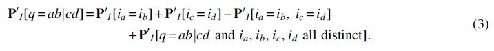$i_{x} \in {1, \dots, I}$ be the ancestral lineage of $x \in {a, b, c, d}$ in R. Then

On the contrary, $\begin{matrix} P'_{I} [q = a c | b d] & \leq P'_{I} [i_{b} \neq i_{a} = i_{c} \neq i_{d}] + P'_{I} [i_{a} \neq i_{b} = i_{d} \neq i_{c}] \\ + P'_{I} [q = a c | b d a n d i_{a}, i_{b}, i_{c}, i_{d} a l l d i s t i n c t], \end{matrix}$ (4)

and similarly for $P'_{I} [q = a c | b d]$ , where note that we double-counted the case $i_{a} = i_{c} \neq i_{d} = i_{b}$ to simplify the expression. By symmetry of the GDL process above R (which holds under $P'_{I}$ ), the last term on the right-hand side (RHS) of (3) and (4) is the same. The same holds for the first two terms on the RHS of (4) this time by the independence and exchangeability of the pairs $(i_{a}, i_{b})$ and $(i_{c}, i_{d})$ under $P'_{I}$ , which further implies $\begin{matrix} P'_{I} [q = a b | c d] - P'_{I} [q = a c | b d] \\ \geq P'_{I} [i_{a} = i_{b}] + P'_{I} [i_{c} = i_{d}] - P'_{I} [i_{a} = i_{b}, i_{c} = i_{d}] - 2 P'_{I} [i_{b} \neq i_{a} = i_{c} \neq i_{d}] \\ = x + y - x y - 2 (1 - x) (1 - y) P'_{I} [i_{a} = i_{c} | i_{a} \neq i_{b}, i_{c} \neq i_{d}] \\ = x + y - x y - 2 (1 - x) (1 - y) P'_{I} [i_{a} = i_{c}] \\ = x + y - x y - 2 (1 - x) (1 - y) \frac{1}{I} \equiv h (x, y) . \end{matrix}$

where $x = P'_{I} [i_{a} = i_{b}]$ and $y = P'_{I} [i_{c} = i_{d}]$ .

For fixed y, $h (x, y)$ is linear in x and $h (1, y) = 1$ . So $h (\cdot, y)$ achieves its minimum at the smallest value allowed for x. The same holds for y. Intuitively, i_a and i_b are “positively correlated” so $x \geq 1 ∕ I$ . We prove this formally next.

Lemma 1. Almost surely, $x, y \geq 1 ∕ I$ .

Proof. For 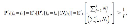$j \in {1, \dots, I}$ , let N_j be the number of gene copies at the most recent common ancestor $R'$ of A and B that descend from copy j in R. Upon conditioning on (N_j) _j , the choice of a and b is independent, with i_a and i_b being picked proportionally to the corresponding N_js (i.e., the gene copies in $R'$ are equally likely to have given rise to a). By the law of total probability and the fact that the quadratic mean is greater than the arithmetic mean,

and similarly for $P'_{I} [i_{c} = i_{d}]$ . □

Returning to the proof of the theorem, evaluating h at $x, y = 1 ∕ I$ gives $h (1 ∕ I, 1 ∕ I) = 2 \frac{1}{I} - \frac{1}{I^{2}} - 2 \frac{{(I - 1)}^{2}}{I^{3}} = \frac{2 I^{2} - I}{I^{3}} - \frac{2 I^{2} - 4 I + 2}{I^{3}} = \frac{3 I - 2}{I^{3}} > 0 .$

That establishes (2) in case 1, which implies $P' [q = a b | c d] > max \{P' [q = a c | b d], P' [q = a d | b c]\},$ (5)

as desired.

The proof in case 2 is similar. Assume that $T^{Q} = (((A, B), C), D)$ , let R be the most recent common ancestor of $A, B, C$ (but not D) in $T^{Q}$ , and let I be the number of gene copies exiting R. As in case 1, it suffices to prove (2) almost surely. Let $i_{x} \in {1, \dots, I}$ be the ancestral lineage of $x \in {a, b, c}$ in R. Then $P'_{I} [q = a b | c d] = P'_{I} [i_{a} = i_{b}] + P'_{I} [q = a b | c d a n d i_{a}, i_{b}, i_{c}, a l l d i s t i n c t] .$ (6)

On the contrary, $P'_{I} [q = a c | b d] = P'_{I} [i_{b} \neq i_{a} = i_{c}] + P'_{I} [q = a c | b d a n d i_{a}, i_{b}, i_{c}, a l l d i s t i n c t],$ (7)

with a similar result for $P'_{I} [q = a d | b c]$ . By symmetry again, the last term on the RHS of (6) and (7) is the same. This implies $\begin{matrix} P'_{I} [q = a b | c d] - P'_{I} [q = a c | b d] = P'_{I} [i_{a} = i_{b}] - P'_{I} [i_{b} \neq i_{a} = i_{c}] \\ = x - (1 - x) P'_{I} [i_{a} = i_{c} | i_{a} \neq i_{b}] = x - (1 - x) \frac{1}{I} \equiv g (x), \end{matrix}$

where $x = P'_{I} [i_{a} = i_{b}]$ . This function g attains its minimum value at the smallest possible of x, which by Lemma 1 is $x = 1 ∕ I$ . Evaluating at $x = 1 ∕ I$ gives $g (1 ∕ I) = \frac{1}{I} - \frac{1}{I} + \frac{1}{I^{2}} = \frac{1}{I^{2}} > 0,$

which establishes (2) in case 2. □

As a direct consequence of our identifiability proof, it is straightforward to establish the statistical consistency of the following pipeline, which we refer to as ASTRAL/ONE [see also Du et al. (2019)]: for each gene tree t_i, pick in each species a random gene copy (if possible) and run ASTRAL on the resulting set of modified gene trees ${\tilde{t}}_{i}$ .

Theorem 2 (Statistical Consistency: ASTRAL/ONE). ASTRAL/ONE is statistically consistent under the GDL model. That is, as the number of input gene trees tends toward infinity, the output of ASTRAL/ONE converges to T almost surely, when run in exact mode or in its default constrained version.

Proof. First, we prove consistency for the exact version of ASTRAL. The input to the ASTRAL/ONE pipeline is the collection of gene trees $T = {t_{i}}_{i = 1}^{k}$ , where t_i is labeled by individuals (i.e., gene copies) $R_{i} \subseteq R$ . For each species and each gene tree t_i, we pick a uniform random gene copy, producing a new gene tree ${\tilde{t}}_{i}$ . Recall that the quartet score of $\tilde{T}$ with respect to $\tilde{T} = {{\tilde{t}}_{i}}_{i = 1}^{k}$ is then

We note that the score only depends on the unrooted topology of $\tilde{T}$ . Under the GDL model, by independence of the gene trees (and non-negativity), $Q_{k} (\tilde{T}) ∕ k$ converges almost surely to its expectation simultaneously for all unrooted species tree topologies over S.

For a species 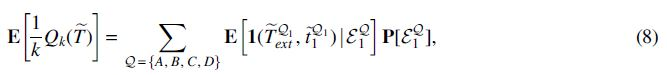$A \in S$ and gene tree ${\tilde{t}}_{i}$ , let A_i be the gene copy in A on ${\tilde{t}}_{i}$ if it exists and let $ℰ_{i}^{A}$ be the event that it exists. For a 4-tuple of species $Q = {A, B, C, D}$ , let $Q_{i} = {A_{i}, B_{i}, C_{i}, D_{i}}$ and $ℰ_{i}^{Q} = ℰ_{i}^{A} \cap ℰ_{i}^{B} \cap ℰ_{i}^{C} \cap ℰ_{i}^{D}$ . The expectation can then be written as

as, on the event , there is no contribution from $Q$ in the sum over the first sample.

Based on the proof of Theorem 1, a different way to write $E [1 ({\tilde{T}}_{e x t}^{Q_{1}}, {\tilde{t}}_{1}^{Q_{1}}) | ℰ_{1}^{Q}]$ is in terms of the original gene tree t₁. Let $a, b, c, d$ be random gene copies on t₁ in $A, B, C, D$ , respectively. Then if q is the topology of t₁ restricted to $a, b, c, d$ , $E [1 ({\tilde{T}}_{e x t}^{Q_{1}}, {\tilde{t}}_{1}^{Q_{1}}) | ℰ_{1}^{Q}] = P' [q = {\tilde{T}}^{Q}] .$

From (5), we know that this expression is maximized (strictly) at the true species tree $P' [q = T^{Q}] .$ Hence, together with (8) and the law of large numbers, almost surely the quartet score is eventually maximized by the true species tree as $k \to + \infty$ . This completes the proof for the exact version.

The default version is statistically consistent for the same reason as in the proof of Theorem 3. As the number of MUL-trees sampled tends to infinity, the true species tree will appear as one of the input gene trees almost surely. So ASTRAL returns the true species tree topology almost surely as the number of sampled MUL-trees increases. □

3.3. Statistical consistency of ASTRAL-multi under GDL

The following consistency result is not a direct consequence of our identifiability result, although the ideas used are similar.

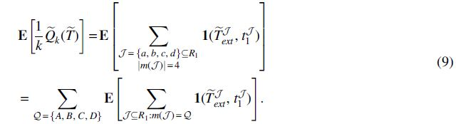
Theorem 3 (Statistical Consistency: ASTRAL-multi). ASTRAL-multi, where copies of a gene in a species are treated as multiple alleles within the species, is statistically consistent under the GDL model. That is, as the number of input gene trees tends toward infinity, the output of ASTRAL-multi converges to T almost surely, when run in exact mode or in its default constrained version.

Proof. First, we show that ASTRAL-multi is consistent when run in exact mode. The input are the gene trees 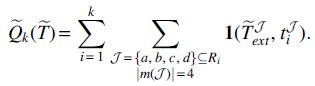$T = {t_{i}}_{i = 1}^{k}$ with t_i labeled by individuals (i.e., gene copies) $R_{i} \subseteq R$ . Then the quartet score of $\tilde{T}$ with respect to $T$ is given by (1). For any 4-tuple of gene copies $J = {a, b, c, d}$ , we define $m (J)$ to be the corresponding set of species. It was proved in Rabiee et al. (2019) that those $J$ s with fewer than 4 species contribute equally to all species tree topologies. As a result, it suffices to work with a modified quartet score

By independence of the gene trees (and non-negativity), ${\tilde{Q}}_{k} (\tilde{T}) ∕ k$ converges almost surely to its expectation simultaneously for all unrooted species tree topologies over S.

The expectation can be simplified as

Let $N_{A B | C D}^{Q}$ (respectively $N_{A C | B D}^{Q}$ , $N_{A D | B C}^{Q}$ ) be the number of choices consisting of one gene copy in t₁ from each species in $Q$ whose corresponding restriction $t_{1}^{Q}$ agrees with $A B | C D$ (respectively $A C | B D$ , $A D | B C$ ). Then each summand in (9) may be written as $E [N_{{\tilde{T}}^{Q}}^{Q}]$ . We establish below that this last expression is maximized at the true species tree $T^{Q}$ , that is, $E [N_{A B | C D}^{Q}] > max \{E [N_{A C | B D}^{Q}], E [N_{A D | B C}^{Q}]\},$ (10)

when (without loss of generality) $T^{Q} = A B | C D$ . From (9) and the law of large numbers, it will then follow that almost surely the quartet score is eventually maximized by the true species tree as $k \to + \infty$ .

It remains to establish (10). Fix $Q = {A, B, C, D}$ a set of four distinct species in T. Assume that the corresponding unrooted quartet topology in T is $A B | C D$ . Let t₁ be an MUL-tree generated under the GDL model over T. Again, there are two cases: $T^{Q}$ is [1] balanced or [2] a caterpillar.

In case 1, let R be the most recent common ancestor of $Q$ in T and let I be the number of gene copies exiting (forward in time) R. For $j \in {1, \dots, I}$ , let $A_{j}$ be the number of gene copies in A descending from j in R, and similarly define $ℬ_{j}$ , $C_{j}$ , and $D_{j}$ . By the law of total probability, $E [N_{A B | C D}^{Q}] = E [E_{I} [N_{A B | C D}^{Q}]] .$ We show that almost surely, $E_{I} [N_{A B | C D}^{Q}] > max \{E_{I} [N_{A C | B D}^{Q}], E_{I} [N_{A D | B C}^{Q}]\},$ (11)

which implies (10). By symmetry, we have $X^{=} \equiv E_{I} [A_{j} ℬ_{j}] = E_{I} [A_{1} ℬ_{1}]$ , $Y^{=} \equiv E_{I} [C_{j} D_{j}] = E_{I} [C_{1} D_{1}]$ , $X^{\neq} \equiv E_{I} [A_{j} ℬ_{k}] = E_{I} [A_{1}] E_{I} [ℬ_{1}]$ , as well as $Y^{\neq} \equiv E_{I} [C_{j} D_{k}] = E_{I} [C_{1}] E_{I} [D_{1}]$ , for all $j, k$ with $j \neq k$ . Hence, the expected number of pairs consisting of a single gene copy from A and B is $X = I X^{=} + I (I - 1) X^{\neq}$ . Arguing similarly to (3) and (4), $\begin{matrix} E_{I} [N_{A B | C D}^{Q}] - E_{I} [N_{A C | B D}^{Q}] \\ \geq (I X^{=}) Y + X (I Y^{=}) - (I X^{=}) (I Y^{=}) - I (I - 1) X^{\neq} [2 (I - 1) Y^{\neq}] \\ = X Y [x + y - x y - 2 (1 - x) (1 - y) \frac{1}{I}], \end{matrix}$

where here we define $x = \frac{I X^{=}}{X}, y = \frac{I Y^{=}}{Y} .$ Following the argument in the proof of Theorem 1, to establish (11) it suffices to show that almost surely, $x, y \geq 1 ∕ I$ . That is implied by the following positive correlation result.

Lemma 2. Almost surely, $X^{=} \geq X^{\neq}$ .

Indeed, we then have: $x = \frac{I X^{=}}{I X^{=} + I (I - 1) X^{\neq}} \geq \frac{I X^{=}}{I X^{=} + I (I - 1) X^{=}} = \frac{1}{I} .$

Proof of Lemma 2. For $j \in {1, \dots, I}$ , let N_j be the number of gene copies at the divergence of the most recent common ancestor of A and B that are descending from j in R. Then, for $j \in {1, \dots, I}$ , since $A_{j}$ and $ℬ_{j}$ are conditionally independent given (N_j) _j under $E_{I}$ , it follows that

where $α$ (respectively $β$ ) is the expected number of gene copies in A (respectively B) descending from a single gene copy in the most recent common ancestor of A and B under $E_{I} .$ Similarly, for $j \neq k \in {1, \dots, I}$ ,

by Cauchy-Schwarz and $E_{I} [N_{j}^{2}] = E_{I} [N_{k}^{2}]$ . □

We now establish (11) in case 2. Assume that $T^{Q} = (((A, B), C), D)$ and let R be the most recent common ancestor of $A, B, C$ (but not D) in T. For $i = 1, 2, 3$ , let $N_{A B | C D}^{Q, {i}}$ (respectively $N_{A C | B D}^{Q, {i}}$ ) be the number of choices consisting of one gene copy from each species in $Q$ whose corresponding restriction on $t^{Q}$ agrees with $A B | C D$ (respectively $A C | B D$ ) and where, in addition, copies of $A, B, C$ descend from i distinct lineages in R. We make five observations:

Contributions to $N_{A B | C D}^{Q, {2}}$ necessarily come from copies in A and B descending from the same lineage in R, together with a copy in C descending from a distinct lineage and any copy in D. Similarly for $N_{A C | B D}^{Q, {2}}$

Moreover, $N_{A C | B D}^{Q, {1}} = 0$ almost surely, as in that case the corresponding copies from A and B coalesce (backward in time) below R.

Arguing as in the proof of Theorem 1, by symmetry we have the equality $E_{I} [N_{A B | C D}^{Q, {3}}] = E_{I} [N_{A C | B D}^{Q, {3}}] .$

For $j \in {1, \dots, I}$ , let $A_{j}$ be the number of gene copies in A descending from j in $R,$ and similarly define $ℬ_{j}$ , $C_{j}$ . Let $D$ be the number of gene copies in D. Then, under the conditional probability $P_{I}$ , $D$ is independent of . Moreover, under P_I, is independent of .

Similarly to case 1, by symmetry we have $X^{=} \equiv E_{I} [A_{j_{1}} ℬ_{j_{1}}] = E_{I} [A_{1} ℬ_{1}]$ , $X^{\neq} \equiv E_{I} [A_{j_{1}} ℬ_{k_{1}}] = E_{I} [A_{1}] E_{I} [ℬ_{1}]$ for all $j_{1}, k_{1}$ with $j_{1} \neq k_{1}$ . Define also $X = I X^{=} + I (I - 1) X^{\neq}$ , $Y \equiv E_{I} [C_{1}]$ , and $Z \equiv E_{I} [D]$ .

Putting these observations together, we obtain $\begin{matrix} E_{I} [N_{A B | C D}^{Q}] - E_{I} [N_{A C | B D}^{Q}] \\ = E_{I} [N_{A B | C D}^{Q, {1}}] + E_{I} [N_{A B | C D}^{Q, {2}}] - E_{I} [N_{A C | B D}^{Q, {2}}] \\ = I X^{=} Y Z + I (I - 1) X^{=} Y Z - I (I - 1) X^{\neq} Y Z \\ > 0, \end{matrix}$

where we used Lemma 2 on the last line.

Thus, ASTRAL-multi is statistically consistent when run in exact mode, because it is guaranteed to return the optimal tree, and that is realized by the species tree. To see why the default version of ASTRAL-multi is also statistically consistent, note that the true species tree will appear as one of the input gene trees, almost surely, as the number of MUL-trees sampled tends to infinity. For instance, the probability of observing no duplications or losses is strictly positive. Furthermore, when this happens, the true species tree bipartitions are all contained in the constraint set $Σ$ used by the default version. Hence, as the number of sampled MUL-trees increases, almost surely ASTRAL-multi will return the true species tree topology. □

4. Experiments

We performed a simulation study to evaluate ASTRAL-multi and other species tree estimation methods on 16-taxon data sets with model conditions characterized by three GDL rates, five levels of GTEE, and four numbers of genes. We briefly describe the study here and provide details sufficient to reproduce the study in Appendix A1. In addition, all scripts and data sets used in this study are available on the Illinois Data Bank: https://doi.org/10.13012/B2IDB-2626814_V1.

Our simulation protocol uses parameters estimated from the 16-taxon fungal data set studied by Du et al. (2019) and Rasmussen and Kellis (2012). First, we used the species tree and other parameters estimated from the fungal data set to simulate gene trees under the DLCoal (Rasmussen and Kellis, 2012) model with three GDL rates (the lowest rate $1 \times 1 0^{- 10}$ reflects the GDL rate estimated from the fungal data set, so that the two higher rates reflect more challenging model conditions). Specifically, for each GDL rate, we simulated 10 replicate data sets (each with 1000 model gene trees that deviated from the strict molecular clock) using SimPhy (Mallo et al., 2016). Although we simulated gene trees under a unified model of GDL and ILS, there was effectively no ILS in our simulated data sets (Table 4 in Appendix A1). Second, for each model gene tree, we used INDELible (Fletcher and Yang, 2009) to simulate a multiple sequence alignment under the GTR+GAMMA model with parameters based on the fungal data set. Third, we ran RAxML (Stamatakis, 2014) to estimate a gene tree under the GTR+GAMMA model from each gene alignment. By varying the length of each gene alignment, four model conditions were created with 23% to 65% mean GTEE, as measured by the normalized Robinson-Foulds (RF) distance (Robinson and Foulds, 1981) between true and estimated gene trees, averaged across all gene trees. Fourth, we ran species tree estimation methods given varying numbers of gene trees as input. Finally, we evaluated species tree error as the normalized RF distance between true and estimated species trees.

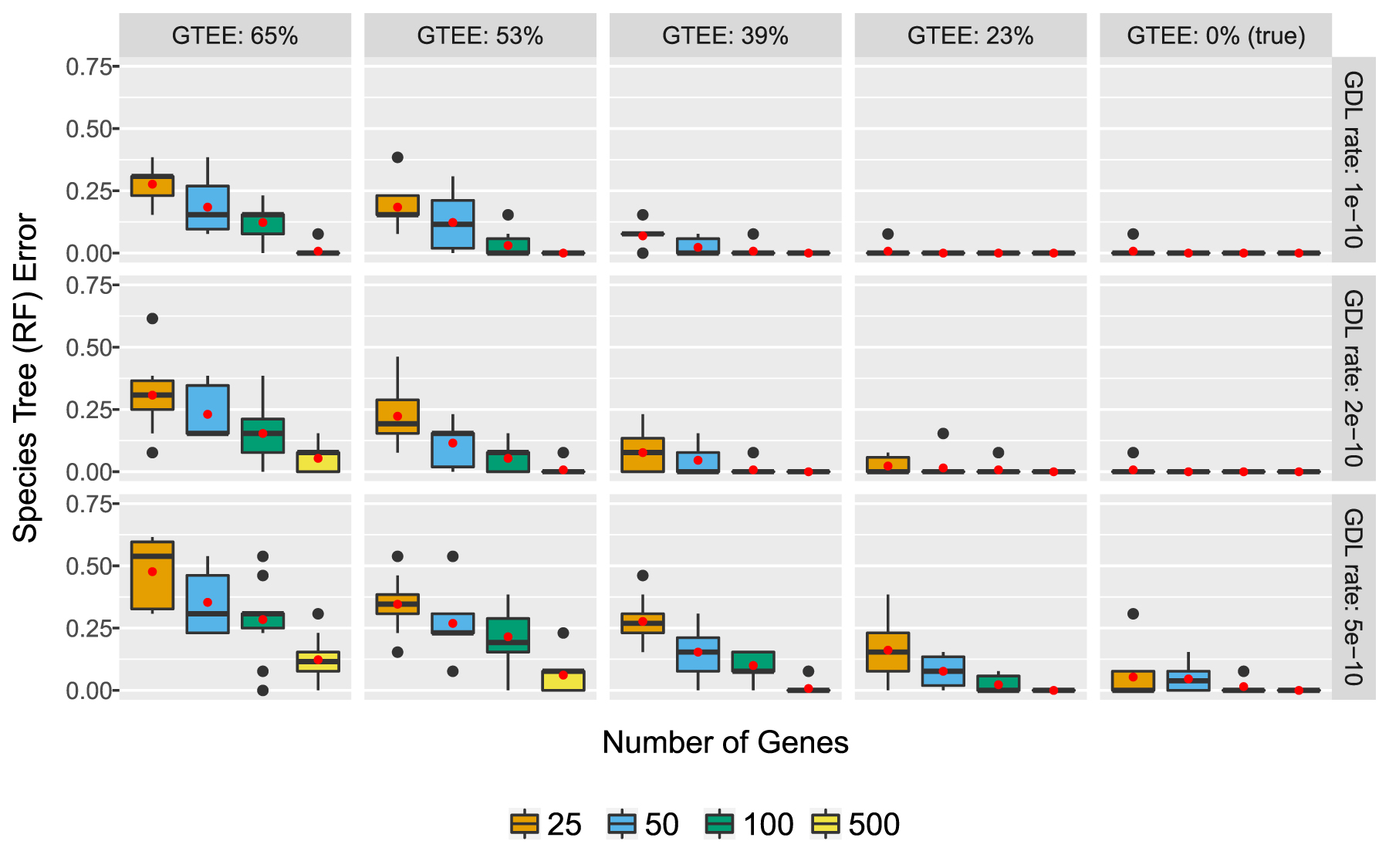
In our first experiment, we explored ASTRAL-multi on both true and estimated gene trees (Fig. 1). ASTRAL-multi was very accurate on true gene trees; even with just 25 true gene trees, the average species tree error was less than 1% for the two lower GDL rates and was less than 6% for the highest GDL rate ( $5 \times 1 0^{- 10}$ ). As expected, species tree error increased with the GDL rate, increased with the GTEE level, and decreased with the number of genes.

FIG. 1.

ASTRAL-multi on true and estimated gene trees generated from the fungal species tree (16 taxa) under a GDL model using three different rates (subplot rows). Estimated gene trees had four different levels of GTEE, by varying the sequence length (subplot columns). We report the average RF error rate between the true and estimated species trees. There are 10 replicate data sets per model condition. Red dots indicate means, and bars indicated medians. GDL, gene duplication and loss; GTEE, gene tree estimation error; RF, Robinson-Foulds.

In our second experiment, we compared ASTRAL-multi to four other species tree methods [DupTree (Wehe et al., 2008), MulRF (Chaudhary et al., 2014), STAG (Emms and Kelly, 2018), and ASTRID-multi, which is ASTRID (Vachaspati and Warnow, 2015) run under the multiallele setting] that take gene trees as input. Figure 2 shows species tree error for model conditions with mean GTEE of 53%. As expected, the error increased for all methods with the GDL rate and GTEE level, and decreased with the number of genes. Differences between methods depended on the model condition. When given 500 genes, all five methods were competitive (with a slight disadvantage to STAG); a similar trend was observed when methods were given 100 genes provided that the GDL rate was one of the two lower rates. When given 50 genes, ASTRAL-multi, MulRF, and ASTRID-multi were the best methods for the two lower GDL rates. On the remaining model conditions, ASTRID-multi was the best method. Finally, STAG was unable to run on some data sets when the GDL rate was high and the number of genes was low; this result was due to STAG failing when none of the input gene trees included at least one copy of every species. Results for other GTEE levels are provided in Tables 1, 2, and 3, and show similar trends.

FIG. 2.

Average RF tree error rates of species tree methods on estimated gene trees (mean GTEE: 53%) generated from the fungal 16-taxon species tree using three different GDL rates (subplot rows) and different numbers of genes (subplot columns). STAG failed to run on some replicate data sets for model conditions indicated by “NA,” because none of the input gene trees included at least one copy of every species.

Table 1.

For Each Model Condition (with Gene Duplication and Loss Rate $1 \times 1 0^{- 10}$ ), Species Tree Error (Mean $\pm$ Standard Deviation Across 10 Replicate Data Sets) Is Shown for Five Different Methods

No. of genes	ASTRAL-multi	MulRF	DupTree	STAG	ASTRID
GDL rate: $1 \times 1 0^{- 10}$ , mean GTEE: 65%
25	$0.28 \pm 0.06$	$0.22 \pm 0.10$	$0.49 \pm 0.19$	$0.39 \pm 0.11$	$0.21 \pm 0.07$
50	$0.18 \pm 0.10$	$0.12 \pm 0.07$	$0.45 \pm 0.11$	$0.24 \pm 0.07$	$0.14 \pm 0.08$
100	$0.12 \pm 0.06$	$0.06 \pm 0.06$	$0.25 \pm 0.11$	$0.15 \pm 0.10$	$0.05 \pm 0.05$
500	$0.01 \pm 0.02$	$0.00 \pm 0.00$	$0.08 \pm 0.10$	$0.02 \pm 0.05$	$0.00 \pm 0.00$
GDL rate: $1 \times 1 0^{- 10}$ , mean GTEE: 39%
25	$0.07 \pm 0.04$	$0.03 \pm 0.04$	$0.11 \pm 0.12$	$0.13 \pm 0.08$	$0.06 \pm 0.06$
50	$0.02 \pm 0.04$	$0.02 \pm 0.04$	$0.09 \pm 0.10$	$0.06 \pm 0.05$	$0.03 \pm 0.04$
100	$0.01 \pm 0.02$	$0.01 \pm 0.02$	$0.02 \pm 0.05$	$0.02 \pm 0.04$	$0.01 \pm 0.02$
500	$0.00 \pm 0.00$	$0.00 \pm 0.00$	$0.00 \pm 0.00$	$0.00 \pm 0.00$	$0.00 \pm 0.00$
GDL rate: $1 \times 1 0^{- 10}$ , mean GTEE: 23%
25	$0.01 \pm 0.02$	$0.01 \pm 0.02$	$0.02 \pm 0.03$	$0.06 \pm 0.06$	$0.00 \pm 0.00$
50	$0.00 \pm 0.00$	$0.00 \pm 0.00$	$0.01 \pm 0.02$	$0.01 \pm 0.02$	$0.00 \pm 0.00$
100	$0.00 \pm 0.00$	$0.00 \pm 0.00$	$0.00 \pm 0.00$	$0.01 \pm 0.02$	$0.00 \pm 0.00$
500	$0.00 \pm 0.00$	$0.00 \pm 0.00$	$0.00 \pm 0.00$	$0.00 \pm 0.00$	$0.00 \pm 0.00$
GDL rate: $1 \times 1 0^{- 10}$ , mean GTEE: 0%
25	$0.01 \pm 0.02$	$0.00 \pm 0.00$	$0.00 \pm 0.00$	$0.00 \pm 0.00$	$0.00 \pm 0.00$
50	$0.00 \pm 0.00$	$0.00 \pm 0.00$	$0.00 \pm 0.00$	$0.00 \pm 0.00$	$0.00 \pm 0.00$
100	$0.00 \pm 0.00$	$0.00 \pm 0.00$	$0.00 \pm 0.00$	$0.00 \pm 0.00$	$0.00 \pm 0.00$
500	$0.00 \pm 0.00$	$0.00 \pm 0.00$	$0.00 \pm 0.00$	$0.00 \pm 0.00$	$0.00 \pm 0.00$

Species tree error was measured as the normalized RF distance between true and estimated species trees.

GDL, gene duplication and loss; GTEE, gene tree estimation error; RF, Robinson-Foulds.

Table 2.

For Each Model Condition (with Gene Duplication and Loss Rate $2 \times 1 0^{- 10}$ ), Species Tree Error (Mean $\pm$ Standard Deviation Across 10 Replicate Data Sets) Is Shown for Five Different Methods

No. of genes	ASTRAL-multi	MulRF	DupTree	STAG	ASTRID
GDL rate: $2 \times 1 0^{- 10}$ , mean GTEE: 65%
25	$0.31 \pm 0.14$	$0.28 \pm 0.10$	$0.53 \pm 0.19$	$0.56 \pm 0.15$	$0.14 \pm 0.10$
50	$0.23 \pm 0.10$	$0.21 \pm 0.11$	$0.39 \pm 0.16$	$0.45 \pm 0.12$	$0.08 \pm 0.07$
100	$0.15 \pm 0.12$	$0.11 \pm 0.09$	$0.33 \pm 0.16$	$0.26 \pm 0.10$	$0.05 \pm 0.08$
500	$0.05 \pm 0.05$	$0.00 \pm 0.00$	$0.13 \pm 0.09$	$0.05 \pm 0.06$	$0.01 \pm 0.02$
GDL rate: $2 \times 1 0^{- 10}$ , mean GTEE: 39%
25	$0.08 \pm 0.08$	$0.12 \pm 0.09$	$0.11 \pm 0.05$	$0.29 \pm 0.15$	$0.08 \pm 0.07$
50	$0.05 \pm 0.06$	$0.03 \pm 0.05$	$0.05 \pm 0.04$	$0.15 \pm 0.14$	$0.02 \pm 0.05$
100	$0.01 \pm 0.02$	$0.00 \pm 0.00$	$0.03 \pm 0.05$	$0.09 \pm 0.08$	$0.01 \pm 0.02$
500	$0.00 \pm 0.00$	$0.00 \pm 0.00$	$0.00 \pm 0.00$	$0.00 \pm 0.00$	$0.00 \pm 0.00$
GDL rate: $2 \times 1 0^{- 10}$ , mean GTEE: 23%
25	$0.02 \pm 0.04$	$0.02 \pm 0.04$	$0.04 \pm 0.05$	$0.11 \pm 0.08$	$0.02 \pm 0.03$
50	$0.02 \pm 0.05$	$0.00 \pm 0.00$	$0.01 \pm 0.02$	$0.06 \pm 0.05$	$0.00 \pm 0.00$
100	$0.01 \pm 0.02$	$0.00 \pm 0.00$	$0.00 \pm 0.00$	$0.01 \pm 0.02$	$0.00 \pm 0.00$
500	$0.00 \pm 0.00$	$0.00 \pm 0.00$	$0.00 \pm 0.00$	$0.00 \pm 0.00$	$0.00 \pm 0.00$
GDL rate: $2 \times 1 0^{- 10}$ , mean GTEE: 0%
25	$0.01 \pm 0.02$	$0.00 \pm 0.00$	$0.00 \pm 0.00$	$0.00 \pm 0.00$	$0.00 \pm 0.00$
50	$0.00 \pm 0.00$	$0.00 \pm 0.00$	$0.00 \pm 0.00$	$0.00 \pm 0.00$	$0.00 \pm 0.00$
100	$0.00 \pm 0.00$	$0.00 \pm 0.00$	$0.00 \pm 0.00$	$0.00 \pm 0.00$	$0.00 \pm 0.00$
500	$0.00 \pm 0.00$	$0.00 \pm 0.00$	$0.00 \pm 0.00$	$0.00 \pm 0.00$	$0.00 \pm 0.00$

Species tree error was measured as the normalized RF distance between true and estimated species trees.

Table 3.

For Each Model Condition (with Gene Duplication and Loss Rate $5 \times 1 0^{- 10}$ ), Species Tree Error (Mean $\pm$ Standard Deviation Across 10 Replicate Data Sets) Is Shown for Five Different Methods

No. of genes	ASTRAL-multi	MulRF	DupTree	STAG	ASTRID
GDL rate: $5 \times 1 0^{- 10}$ , mean GTEE: 65%
25	$0.48 \pm 0.13$	$0.36 \pm 0.12$	$0.65 \pm 0.09$	$n a n \pm n a n$	$0.34 \pm 0.12$
50	$0.35 \pm 0.13$	$0.30 \pm 0.10$	$0.48 \pm 0.24$	$n a n \pm n a n$	$0.19 \pm 0.15$
100	$0.28 \pm 0.15$	$0.18 \pm 0.08$	$0.36 \pm 0.23$	$0.52 \pm 0.11$	$0.09 \pm 0.08$
500	$0.12 \pm 0.09$	$0.04 \pm 0.04$	$0.20 \pm 0.10$	$0.22 \pm 0.10$	$0.00 \pm 0.00$
GDL rate: $5 \times 1 0^{- 10}$ , mean GTEE: 39%
25	$0.28 \pm 0.09$	$0.25 \pm 0.08$	$0.16 \pm 0.12$	$n a n \pm n a n$	$0.14 \pm 0.07$
50	$0.15 \pm 0.10$	$0.09 \pm 0.07$	$0.06 \pm 0.07$	$n a n \pm n a n$	$0.05 \pm 0.06$
100	$0.10 \pm 0.05$	$0.05 \pm 0.05$	$0.03 \pm 0.05$	$0.28 \pm 0.10$	$0.02 \pm 0.03$
500	$0.01 \pm 0.02$	$0.00 \pm 0.00$	$0.00 \pm 0.00$	$0.06 \pm 0.07$	$0.00 \pm 0.00$
GDL rate: $5 \times 1 0^{- 10}$ , mean GTEE: 23%
25	$0.16 \pm 0.12$	$0.05 \pm 0.04$	$0.05 \pm 0.09$	$n a n \pm n a n$	$0.02 \pm 0.03$
50	$0.08 \pm 0.06$	$0.05 \pm 0.05$	$0.01 \pm 0.02$	$n a n \pm n a n$	$0.01 \pm 0.02$
100	$0.02 \pm 0.04$	$0.03 \pm 0.05$	$0.00 \pm 0.00$	$0.17 \pm 0.11$	$0.00 \pm 0.00$
500	$0.00 \pm 0.00$	$0.00 \pm 0.00$	$0.00 \pm 0.00$	$0.02 \pm 0.03$	$0.00 \pm 0.00$
GDL rate: $5 \times 1 0^{- 10}$ , mean GTEE: 0%
25	$0.05 \pm 0.09$	$0.00 \pm 0.00$	$0.00 \pm 0.00$	$n a n \pm n a n$	$0.01 \pm 0.02$
50	$0.05 \pm 0.05$	$0.00 \pm 0.00$	$0.00 \pm 0.00$	$n a n \pm n a n$	$0.00 \pm 0.00$
100	$0.02 \pm 0.03$	$0.00 \pm 0.00$	$0.00 \pm 0.00$	$0.05 \pm 0.08$	$0.00 \pm 0.00$
500	$0.00 \pm 0.00$	$0.00 \pm 0.00$	$0.00 \pm 0.00$	$0.00 \pm 0.00$	$0.00 \pm 0.00$

Species tree error was measured as the normalized RF distance between true and estimated species trees. nan = NaN (Not a Number).

5. Discussion and Conclusion

This study establishes the identifiability of unrooted species trees under the simple model of GDL from Arvestad et al. (2009) and that ASTRAL-multi is statistically consistent under this model. In our simulation study, ASTRAL-multi was accurate under challenging model conditions, characterized by high GDL rates and high GTEE, provided that a sufficiently large number of genes is given as input. When the number of genes was smaller, ASTRID-multi often had an advantage over ASTRAL-multi and the other methods.

The results of this study can be compared with the previous study by Chaudhary et al. (2015), who also evaluated species tree estimation methods under model conditions with GDL. They found that MulRF and gene tree parsimony methods had better accuracy than NJst (Liu and Yu, 2011) (a method that is similar to ASTRID). Their study has an advantage over our study in that it explored larger data sets (up to 500 species); however, all genes in their study evolved under a strict molecular clock, and they did not evaluate ASTRAL-multi.

Our study is the first study to evaluate ASTRAL-multi on estimated gene trees, and we also explore model conditions with varying levels of GTEE. Evaluating methods under conditions with moderate to high GTEE is critical, as estimated gene trees from four recent studies (Jarvis et al., 2014; Hosner et al., 2016; Streicher et al., 2016; Blom et al., 2017) all had mean bootstrap support values below 50% [see table 1 in Molloy and Warnow (2018)], suggesting high GTEE.

Our study is limited to one underlying species tree topology with 16 species. Previous studies (Vachaspati and Warnow, 2016) have shown that MulRF (which uses a heuristic search strategy to find solutions to its NP-hard optimization problem) is much slower than ASTRAL on large data sets, suggesting that ASTRAL-multi may dominate MulRF as the number of species increases. Hence, future studies should investigate ASTRAL-multi and other methods under a broader range of conditions, including larger numbers of species. Future research should also consider empirical performance and statistical consistency under different causes of gene tree heterogeneity.

We note with interest that the proof that ASTRAL-multi is statistically consistent is based on the fact that the most probable unrooted gene tree on four leaves (according to two ways of defining it) under the GDL model is the true species tree (equivalently, there is no anomaly zone for the GDL model for unrooted four-leaf trees). This coincides with the reason ASTRAL is statistically consistent under the MSC as well as under a model for random horizontal gene transfer (HGT) (Roch and Snir, 2013; Daskalakis and Roch, 2016). Furthermore, previous studies have shown that ASTRAL has good accuracy in simulation studies where both ILS and HGT are present (Davidson et al., 2015). Hence ASTRAL, which was originally designed for species tree estimation in the presence of ILS, has good accuracy and theoretical guarantees under different sources of gene tree heterogeneity.

We also note the surprising accuracy of DupTree, MulRF, and ASTRID-multi, methods that, like ASTRAL-multi, are not based on likelihood under a GDL model. Therefore, DynaDup (Mirarab, 2019; Bayzid and Warnow, 2018) is also of potential interest, as it is similar to DupTree in seeking a tree that minimizes the duploss score (although the score is modified to reflect true biological loss), but has the potential to scale to larger data sets via its use of dynamic programming to solve the optimization problem in polynomial time within a constrained search space. In addition, future research should explore these methods compared with more computationally intensive methods such as InferNetwork_ML and InferNetwork_MPL [maximum likelihood and maximum pseudolikelihood methods in PhyloNet (Than et al., 2008; Wen et al., 2018)] restricted so that they produce trees rather than reticulate phylogenies, or PHYLDOG (Boussau et al., 2013) a likelihood-based method for coestimating gene trees and the species tree under a GDL model.

6. Appendices

6.1. Appendix A1: Details of simulation study

All scripts and data sets used in this study are available on the Illinois Data Bank: https://doi.org/10.13012/B2IDB-2626814_V1.

6.1.1. Simulation

Our simulation protocol is (largely) based on the 16-taxon fungal data set from Rasmussen and Kellis (2012).

6.1.1.1. Gene tree simulation

First, we used the species tree estimated by Rasmussen and Kellis (2012) (download: http://compbio.mit.edu/dlcoal/pub/config/fungi.stree) as the model species tree, modifying the branch lengths to be ultrametric and in generations, assuming 10 generations per year. Below is the Newick string for the resulting model species tree (height: 1,800,000,337.5 generations).

(((((((scer: 70617600.0, spar: 70617600.0): 49996800.0, smik: 120614400.0): 59706000.0, sbay: 180320400.0): 526823100.0, cgla: 707143500.0): 72206550.0, scas: 779350050.0): 231815475.0, ((agos: 785532600.0, klac: 785532600.0): 104349600.0, kwal: 889882200.0): 121283325.0): 788834812.5, (((calb: 412758000.0, ctro: 412758000.0): 296329500.0, (cpar:523231200.0, lelo: 523231200.0): 185856300.0): 311495850.0, ((cgui: 756158400.0, dhan: 756158400.0): 140068800.0, clus: 896227200.0): 124356150.0): 779416987.5);

We then simulated gene trees from this model species tree under the DLCoal model (Rasmussen and Kellis, 2012) (a unified model of GDL and ILS) with three different GDL rates using SimPhy Version 1.0.2 with the command:

simphy-1.0.2-mac64 -rs $nreps -rl F:ngens -rg 1 -s $stree \

-si F:1 -sp F:$psize -su F:$mrate -sg F:10 -lb F:$drate \

-ld F:lb -hg LN:1.5,1 -o <output directory> -ot 0 -om 1 \

-od 1 -op 1 -oc 1 -ol 1 -v 3 -cs 293745 &> <log file>

where $nreps is the number of replicate data sets (10), $ngens is the number of genes trees per data set (1000), $stree is the model species tree (Newick string above), $psize is the effective population size ( $1 \times 1 0^{7}$ ), $mrate is the tree-wide substitution rate ( $4 \times 1 0^{- 10}$ substitutions per generation per site), and $drate is the duplication rate (either $1 \times 1 0^{- 10}$ , $2 \times 1 0^{- 10}$ , or $5 \times 1 0^{- 10}$ duplication events per generation per lineage). Note that the loss rate always equaled the duplication rate.

These parameters (with the GDL rate of $1 \times 1 0^{- 10}$ ) are similar to those estimated from the fungal data set by Rasmussen and Kellis (2012) and are the same as parameters used in the simulation study by Du et al. (2019)—except that we assumed 10 generations per year instead of $1 . \bar{1}$ generations per year (note that we accidentally used the value estimated for the fly data set instead of the fungal data set; thanks to Céline Scornavacca for pointing this out to us!).

Fortunately, our parameter choice seems reasonable enough given that Rasmussen and Kellis (2012) considered values of 0.6 generations per year up to 10 generations per year for the fungal data set and selected $1 . \bar{1}$ generations per year, suggesting that $1 . \bar{1}$ generations per year (i.e., 0.9 years per generation) resulted in a level of ILS in simulated data sets that was similar to the level of ILS estimated from the biological data set (although it is worth noting that the ILS level can be difficult to estimate in the presence of GTEE).

To understand the impact of our parameter choice, we simulated data sets assuming $1 . \bar{1}$ generations per year. Below is the Newick string for the model species tree (height: 200000037.5 generations) used.

(((((((scer: 7846400.0, spar: 7846400.0): 5555200.0, smik: 13401600.0): 6634000.0, sbay: 20035600.0): 58535900.0, cgla: 78571500.0): 8022950.0, scas: 86594450.0): 25757275.0, ((agos: 87281400.0, klac: 87281400.0): 11594400.0, kwal: 98875800.0): 13475925.0): 87648312.5, (((calb: 45862000.0, ctro: 45862000.0): 32925500.0, (cpar: 58136800.0, lelo: 58136800.0): 20650700.0): 34610650.0, ((cgui: 84017600.0, dhan: 84017600.0): 15563200.0, clus: 99580800.0): 13817350.0): 86601887.5);

From these simulations, we found that assuming $1 . \bar{1}$ generations per year (instead of 10 generations per year) produces data sets with higher ILS levels and lower numbers of duplication/loss events (Table 4), as expected. Furthermore, we found that assuming $1 . \bar{1}$ generations per year produced data sets with very few loci having multiple copies of species—and the proportion of loci was multiple copies far less than what was observed in the biological data set (Appendix A2). In light of this analysis, our parameter choice seems reasonable, but also suggests that future studies should examine model conditions with higher levels of ILS.

Table 4.

We Provide Summary Statistics for the Simulated Data Sets Below

GDL rate	ILS level (AD%)	Mean no. of species (out of 16) per gene tree	Mean no. of leaves per gene tree
Assuming 10 generations per year
$1 \times 1 0^{- 10}$	0.20% $\pm$ 0.03%	13.61 $\pm$ 0.09	16.09 $\pm$ 0.14
$2 \times 1 0^{- 10}$	0.37% $\pm$ 0.07%	12.02 $\pm$ 0.12	16.36 $\pm$ 0.14
$5 \times 1 0^{- 10}$	0.68% $\pm$ 0.14%	9.20 $\pm$ 0.10	17.42 $\pm$ 0.25
Assuming $1 . \bar{1}$ generations per year
$1 \times 1 0^{- 10}$	15.76% $\pm$ 0.44%	15.69 $\pm$ 0.03	16.01 $\pm$ 0.05
$2 \times 1 0^{- 10}$	15.80% $\pm$ 0.35%	15.41 $\pm$ 0.04	16.03 $\pm$ 0.10
$5 \times 1 0^{- 10}$	15.47% $\pm$ 0.55%	14.57 $\pm$ 0.06	16.04 $\pm$ 0.11

All values shown below are averages ( $\pm$ standard deviations) across the 10 replicate data sets for each of the three GDL rates.

We quantify the level of ILS as the normalized RF distance between each true locus tree and its respective true gene tree (which are on the same leaf set), averaged across all 1000 locus/gene trees (we refer to this value as the average distance or AD). Because these values are all less than 1% for the simulation assuming 10 generations per year, there is effectively no ILS in these data sets. The level of ILS is much higher for the simulation assuming $1 . \bar{1}$ generations per year (AD is 15%). While the ILS is higher assuming $1 . \bar{1}$ generations per year, the number of duplication/loss events is lower, as shown by the number of species per gene tree compared with the number of leaves per gene tree, both averaged across all 1000 gene trees. Because the gene duplication and gene loss rates were equal, the number of leaves per locus/gene tree was close to the number of leaves in the species tree. As the GDL rate increased, the number of species per locus/gene tree decreased, and thus, even though locus/gene trees had the same number of leaves on average, these leaves were labeled by fewer species as the GDL rate increased. Note that in the biological data set, the average ( $\pm$ standard deviation) number of species per gene tree was 13.02 $\pm$ 4.13, and the average ( $\pm$ standard deviation) number of leaves per gene tree was 15.41 $\pm$ 8.31.

ILS, incomplete lineage sorting.

Last, unlike in the simulation study by Du et al. (2019), we did not enable gene conversion and allowed gene trees to deviate from the strict molecular clock by using the gene-by-lineage-specific rate heterogeneity modifiers (−hg). This means that a gamma distribution was defined for each gene tree by drawing $α$ from a log-normal distribution with a location of 1.5 and a scale of 1 [same parameters as Zhang et al. (2018)], and then, each branch in a gene tree was multiplied by a value-drawn gamma distribution corresponding to that gene tree.

In summary, we used SimPhy to produce data sets with three model conditions, characterized by the three GDL rates; each of these model conditions had 10 replicate data sets, and each of these replicate data sets had 1000 gene trees.

6.1.1.2. Sequence simulation

For each model gene tree, we simulated a multiple sequence alignment (1000 base pairs) using INDELible Version 1.03 with GTR+GAMMA model parameters drawn from distributions; specifically, GTR base frequencies (A, C, G, T) were drawn from Dirichlet (113.48869, 69.02545, 78.66144, 99.83793), GTR substitution rates (AC, AG, AT, CG, CT, GT) were drawn from Dirichlet (12.776722, 20.869581, 5.647810, 9.863668, 30.679899, 3.199725), and $α$ was drawn from lognormal (−0.470703916, 0.348667224), where the first parameter is the meanlog and the second parameter is the sdlog.

These distributions were based on the fungal data set from Rasmussen and Kellis (2012) (download: http://compbio.mit.edu/dlcoal/pub/data/real-fungi.tar.gz), which included a multiple sequence alignment estimated using MUSCLE (Edgar, 2004) and a maximum likelihood tree estimated using PhyML (Guindon et al., 2010) for each of the 5351 genes. We estimated GTR+GAMMA model parameters using RAxML Version 8.2.12 with the command:

raxmlHPC-SSE3 -m GTRGAMMA -f e -t <PhyML gene tree file> \

-s <MUSCLE alignment file> -n < output name>

We then fit distributions to the parameters estimated from alignments with at least 500 distinct alignment patterns and at most 25% gaps.

6.1.2. Gene tree estimation

On gene trees with four or more species, we estimated gene trees using RAxML Version 8.2.12 with the command:

raxmlHPC-SSE3 -m GTRGAMMA -p < random seed> -n < output name> \

-s <alignment file>

We truncated sequences to the first 25, 50, 100, and 250 base pairs to produce data sets with varying levels of GTEE. Sequence lengths of 25, 50, 100, and 250 resulted in mean GTEE of 65%, 53%, 39%, and 23%, respectively. Mean GTEE was measured as the normalized RF distance between true and estimated gene trees, averaged across all gene trees.

6.1.3. Species tree estimation

We estimated species trees using the first 25, 50, 100, or 500 (true or estimated) gene trees. ASTRAL Version 5.6.3 was run with the command:

java -Xms2000M -Xmx20000M -jar astral.5.6.3.jar -i <gene tree file> \

-a <name map file> -o <output file> &> <log file>

ASTRID Version 2.2.1 was run with the command:

/ASTRID -u -s -i <gene tree file> -a <name map file> \

-o <output file> &> <log file>

DupTree (download: http://genome.cs.iastate.edu/CBL/DupTree/linux-i386.tar.gz) was run with the command:

/duptree -i <gene tree file> -o <output file> &> <log file>

MulRF Version 2.1 was run with the command:

/MulRFSupertreeLin -i <gene tree file> -o <output file> &> <log file>

STAG (download: https://github.com/davidemms/STAG) was run with the command:

python stag.py <name map file> <gene tree folder> &> <log file>

We ran STAG with FastME Version 2.1.5 (Lefort et al., 2015). Importantly, STAG only uses gene trees that include at least one copy of every species. When the level of GDL was high (i.e., $5 \times 1 0^{- 10}$ ), STAG failed to run on 3/10 replicates with 25 genes and 2/10 replicates on 50 genes, because none of the input gene trees included at least one copy of every species; we do not show results using STAG for those model conditions.

6.2. Appendix A2: Statistics on the number of copies per species in data sets

In Tables 5, 6, and 7, we report statistics on the number of copies per species in biological and simulated data sets.

Table 5.

For the Fungal Biological Data Set, We Report the Mean $\pm$ Standard Deviation, the Minimum, and the Maximum Number of Copies of Each Species Across 5351 Gene Trees

Species	Mean $\pm$ Std	Max	$=$ 1	$>$ 1	$>$ 2	$>$ 5	$>$ 10	$>$ 20
Ashbya gossypii	0.85 $\pm$ 0.58	13	0.731	0.050	0.008	0.001	0.000	0.000
Candida albicans	1.04 $\pm$ 0.65	7	0.769	0.111	0.027	0.001	0.000	0.000
Candida glabrata	0.93 $\pm$ 0.81	27	0.667	0.110	0.019	0.002	0.001	0.000
Candida guilliermondii	0.99 $\pm$ 0.70	11	0.722	0.110	0.027	0.001	0.000	0.000
Candida lusitaniae	0.95 $\pm$ 0.62	10	0.728	0.098	0.019	0.000	0.000	0.000
Candida parapsilosis	1.00 $\pm$ 0.73	12	0.729	0.110	0.028	0.003	0.000	0.000
Candida tropicalis	1.04 $\pm$ 0.73	8	0.738	0.122	0.033	0.003	0.000	0.000
Debaryomyces hansenii	1.02 $\pm$ 0.65	7	0.756	0.110	0.026	0.002	0.000	0.000
Kluyveromyces latics	0.89 $\pm$ 0.63	15	0.745	0.063	0.010	0.002	0.000	0.000
Kluyveromyces waltii	0.88 $\pm$ 0.71	18	0.736	0.059	0.011	0.002	0.001	0.000
Lodderomyces elongisporus	0.98 $\pm$ 0.66	9	0.727	0.108	0.021	0.001	0.000	0.000
Saccharomyces bayanus	0.94 $\pm$ 0.81	23	0.643	0.128	0.022	0.002	0.000	0.000
Saccharomyces castellii	1.01 $\pm$ 0.91	25	0.638	0.154	0.028	0.003	0.001	0.000
Saccharomyces cerevisiae	1.03 $\pm$ 1.09	42	0.678	0.141	0.027	0.004	0.001	0.001
Saccharomyces mikatae	0.92 $\pm$ 0.76	18	0.646	0.118	0.021	0.002	0.000	0.000
Saccharomyces paradoxus	0.95 $\pm$ 0.83	25	0.649	0.129	0.023	0.002	0.000	0.000

For each species, we also report the fraction of gene trees with exactly one copy of the species as well as the fraction of gene trees with more than 1, 2, 5, 10, and 20 copies of the species (i.e., $>$ 1 indicates the number of gene trees out of 5351 with more than 1 copy of the species).

Table 6.

For a Data Set (Replicate 1) Simulated from the Estimated Fungal Species Tree Assuming 10 Generations per Year and a Duplication/Loss Rate of $1 \times 1 0^{- 10}$ , We Report the Mean $\pm$ Standard Deviation, the Minimum, and the Maximum Number of Copies of Each Species Across 1000 Gene Trees

Species	Mean $\pm$ Std	Max	$=$ 1	$>$ 1	$>$ 2
A. gossypii	0.99 $\pm$ 0.60	4	0.708	0.130	0.017
C. albicans	1.02 $\pm$ 0.61	5	0.725	0.135	0.027
C. glabrata	0.99 $\pm$ 0.63	4	0.700	0.130	0.024
C. guilliermondii	0.99 $\pm$ 0.53	3	0.753	0.113	0.011
C. lusitaniae	1.01 $\pm$ 0.58	4	0.727	0.131	0.016
C. parapsilosis	1.03 $\pm$ 0.60	5	0.722	0.144	0.015
C. tropicalis	1.03 $\pm$ 0.62	4	0.725	0.136	0.024
D. hansenii	1.00 $\pm$ 0.58	4	0.730	0.125	0.020
K. latics	0.99 $\pm$ 0.60	4	0.695	0.138	0.015
K. waltii	1.00 $\pm$ 0.59	4	0.712	0.132	0.018
L. elongisporus	1.03 $\pm$ 0.59	4	0.729	0.137	0.021
S. bayanus	1.03 $\pm$ 0.64	5	0.688	0.157	0.024
S. castellii	1.00 $\pm$ 0.61	4	0.718	0.126	0.023
S. cerevisiae	1.02 $\pm$ 0.62	5	0.709	0.143	0.022
S. mikatae	1.01 $\pm$ 0.62	5	0.703	0.141	0.023
S. paradoxus	1.02 $\pm$ 0.63	5	0.710	0.140	0.023

Table 7.

For a Data Set (Replicate 1) Simulated from the Estimated Fungal Species Tree Assuming $1 . \bar{1}$ Generations per Year and a Duplication/Loss Rate of $1 \times 1 0^{- 10}$ , We Report the Mean $\pm$ Standard Deviation, the Minimum, and the Maximum Number of Copies of Each Species Across 1000 Gene Trees

Species	Mean $\pm$ Std	Max	$=$ 1	$>$ 1	$>$ 2
A. gossypii	0.99 $\pm$ 0.19	2	0.962	0.016	0.000
C. albicans	1.00 $\pm$ 0.21	3	0.961	0.020	0.002
C. glabrata	1.00 $\pm$ 0.15	2	0.976	0.010	0.000
C. guilliermondii	1.00 $\pm$ 0.21	3	0.957	0.020	0.001
C. lusitaniae	1.00 $\pm$ 0.22	4	0.963	0.018	0.002
C. parapsilosis	1.01 $\pm$ 0.22	3	0.959	0.024	0.003
C. tropicalis	1.00 $\pm$ 0.21	3	0.960	0.020	0.002
D. hansenii	1.01 $\pm$ 0.21	3	0.958	0.024	0.001
K. latics	1.00 $\pm$ 0.19	2	0.964	0.018	0.000
K. waltii	0.99 $\pm$ 0.18	2	0.969	0.011	0.000
L. elongisporus	1.00 $\pm$ 0.22	3	0.956	0.023	0.002
S. bayanus	0.99 $\pm$ 0.16	2	0.974	0.010	0.000
S. castellii	0.99 $\pm$ 0.17	2	0.972	0.007	0.000
S. cerevisiae	0.99 $\pm$ 0.15	2	0.976	0.008	0.000
S. mikatae	0.99 $\pm$ 0.15	2	0.977	0.008	0.000
S. paradoxus	0.99 $\pm$ 0.16	2	0.974	0.008	0.000

Footnotes

Acknowledgments

All computational analyses were performed on the Illinois Campus Cluster and the Blue Waters supercomputer, computing resources that are operated and financially supported by UIUC in conjunction with the National Center for Supercomputing Applications.

Author Disclosure Statement

The authors declare they have no competing financial interests.

Funding Information

This study was supported, in part, by NSF grants CCF-1535977 and 1513629 (to T.W.) and by the Ira and Debra Cohen Graduate Fellowship in Computer Science (to E.K.M.). SR was supported by NSF grants DMS-1614242, CCF-1740707 (TRIPODS), and DMS-1902892, as well as a Simons Fellowship and a Vilas Associates Award. BL was supported by NSF grants DMS-1614242 (to S.R.) and CCF-1740707. Blue Waters is supported by the NSF (grants OCI-0725070 and ACI-1238993) and the state of Illinois.

References

Allman

E.S.

, Degnan

J.H.

, and Rhodes

J.A.

2011. Identifying the rooted species tree from the distribution of unrooted gene trees under the coalescent. J. Math. Biol. 62, 833–862.

Arvestad

, Lagergren

, and Sennblad

2009. The gene evolution model and computing its associated probabilities. J. ACM 56, Article no. 7.

Bandelt

H.-J.

, and Dress

1986. Reconstructing the shape of a tree from observed dissimilarity data. Adv. Appl. Math. 7, 309–343.

Bansal

M.S.

, Burleigh

J.G.

, Eulenstein

, et al. 2010. Robinson-Foulds supertrees. Algorithms Mol. Biol. 5, Article no. 18.

Bayzid

M.S.

, and Warnow

2018. Gene tree parsimony for incomplete gene trees: Addressing true biological loss. Algorithms Mol. Biol. 13, Article no. 1.

Blom

M.P.K.

, Bragg

J.G.

, Potter

, et al. 2017. Accounting for uncertainty in gene tree estimation: summary-coalescent species tree inference in a challenging radiation of Australian lizards. Syst. Biol. 66, 352–366.

Boussau

, Szöllősi

G.J.

, Duret

, et al. 2013. Genome-scale coestimation of species and gene trees. Genome Res. 23, 323–330.

Chaudhary

, Fernández-Baca

, and Burleigh

J.G.

2014. MulRF: A software package for phylogenetic analysis using multi-copy gene trees. Bioinformatics, 31, 432–433.

Chaudhary

, Boussau

, Burleigh

J.G.

, et al. 2015. Assessing approaches for inferring species trees from multi-copy genes. Syst. Biol. 64, 325–339.

10.

Daskalakis

, and Roch

2016. Species trees from gene trees despite a high rate of lateral genetic transfer: A tight bound (extended abstract), 1621–1630. In Proceedings of the Twenty-Seventh Annual ACM-SIAM Symposium on Discrete Algorithms. Arlington, Virginia, USA.

11.

Davidson

, Vachaspati

, Mirarab

, et al. 2015. Phylogenomic species tree estimation in the presence of incomplete lineage sorting and horizontal gene transfer. BMC Genomics, 16, S1.

12.

, Hahn

M.W.

, and Nakhleh

2019. Species tree inference under the multispecies coalescent on data with paralogs is accurate. DOI: 10.1101/498378. bioRxiv.

13.

Edgar

R.C.

2004. MUSCLE: Multiple sequence alignment with high accuracy and high throughput. Nucleic Acids Res. 32, 1792–1797.

14.

Emms

, and Kelly

2018. STAG: Species tree inference from all genes. DOI: 10.1101/267914. bioRxiv.

15.

Fletcher

, and Yang

2009. INDELible: A flexible simulator of biological sequence evolution. Mol. Biol. Evol. 26, 1879–1888.

16.

Guindon

, Dufayard

J.-F.

, Lefort

, et al. 2010. New algorithms and methods to estimate maximum-likelihood phylogenies: Assessing the performance of PhyML 3.0. Syst. Biol. 59, 307–321.

17.

Hill

, Legried

, and Roch

2020. Species tree estimation under joint modeling of coalescence and duplication: Sample complexity of quartet methods. Available at http://arxiv.org/abs/2007.06697. Accessed July 2020 .

18.

Hosner

P.A.

, Faircloth

B.C.

, Glenn

T.C.

, et al. 2016. Avoiding missing data biases in phylogenomic inference: An empirical study in the landfowl (Aves: Galliformes). Mol. Biol. Evol. 33, 1110–1125.

19.

Jarvis

E.D.

, Mirarab

, Aberer

A.J.

, et al. 2014. Whole-genome analyses resolve early branches in the tree of life of modern birds. Science, 346, 1320–1331.

20.

Kingman

J.F.C.

1982. The coalescent. Stoch. Process. Their Appl. 13, 235–248.

21.

Larget

B.R.

, Kotha

S.K.

, Dewey

C.N.

, et al. 2010. BUCKy: Gene tree/species tree reconciliation with bayesian concordance analysis. Bioinformatics, 26, 2910–2911.

22.

Lefort

, Desper

, and Gascuel

2015. FastME 2.0: A comprehensive, accurate, and fast distance-based phylogeny inference program. Mol. Biol. Evol. 32, 2798–2800.

23.

Legried

, Molloy

E.K.

, Warnow

, et al. 2020. Polynomial-time statistical estimation of species trees under gene duplication and loss, 120–135. In Schwartz, R., ed. Research in Computational Molecular Biology, Lecture Notes in Computer Science. Springer International Publishing, Cham.

24.

Liu

, and Yu

2011. Estimating species trees from unrooted gene trees. Syst. Biol. 60, 661–667.

25.

Maddison

1997. Gene trees in species trees. Syst. Biol. 46, 523–536.

26.

Mallo

, De Oliveira Martins

, and Posada

2016. SimPhy: Phylogenomic simulation of gene, locus, and species trees. Syst. Biol. 65, 334–344.

27.

Markin

, and Eulenstein

2020. Quartet-based inference methods are statistically consistent under the unified duplication-loss-coalescence model. Avialable at http://arxiv.org/abs/2004.04299. Accessed April 2020 .

28.

Mirarab

2019. DynaDup Github Repository: A software package for species tree estimation from rooted gene trees under gene duplication and loss. Avaiable at https://github.com/smirarab/DynaDup. Accessed October 3, 2019.

29.

Mirarab

, Reaz

, Bayzid

M.S.

, et al. 2014. ASTRAL: Genome-scale coalescent-based species tree estimation. Bioinformatics, 30, i541–i548.

30.

Mirarab

, and Warnow

2015. ASTRAL-II: Coalescent-based species tree estimation with many hundreds of taxa and thousands of genes. Bioinformatics, 31, i44–i52.

31.

Molloy

E.K.

, and Warnow

2018. To include or not to include: The impact of gene filtering on species tree estimation methods. Syst. Biol. 67, 285–303.

32.

Rabiee

, Sayyari

, and Mirarab

2019. Multi-allele species reconstruction using ASTRAL. Mol. Phylogenet. Evol. 130, 286–296.

33.

Rasmussen

M.D.

, and Kellis

2012. Unified modeling of gene duplication, loss, and coalescence using a locus tree. Genome Res. 22, 755–765.

34.

Robinson

, and Foulds

1981. Comparison of phylogenetic trees. Math. Biosci. 53, 131–147.

35.

Roch

, Nute

, and Warnow

2018. Long-branch attraction in species tree estimation: Inconsistency of partitioned likelihood and topology-based summary methods. Syst. Biol. 68, 281–297.

36.

Roch

, and Snir

2013. Recovering the treelike trend of evolution despite extensive lateral genetic transfer: A probabilistic analysis. J. Comput. Biol. 20, 93–112.

37.

Roch

, and Steel

2015. Likelihood-based tree reconstruction on a concatenation of aligned sequence data sets can be statistically inconsistent. Theor. Popul. Biol. 100, 56–62.

38.

Stamatakis

2014. RAxML Version 8: A tool for phylogenetic analysis and post-analysis of large phylogenies. Bioinformatics, 30, 1312–1313.

39.

Streicher

J.W.

, Schulte

, J.A., and Wiens

J.J.

2016. How should genes and taxa be sampled for phylogenomic analyses with missing data? An empirical study in iguanian lizards. Syst. Biol. 65, 128–145.

40.

Takahata

1989. Gene genealogy in three related populations: Consistency probability between gene and population trees. Genetics, 122, 957–966.

41.

Than

, Ruths

, and Nakhleh

2008. PhyloNet: A software package for analyzing and reconstructing reticulate evolutionary relationships. BMC Bioinformatics 9, Article no. 322.

42.

Vachaspati

, and Warnow

2015. ASTRID: Accurate species TRees from internode distances. BMC Genomics, 16, S3.

43.

Vachaspati

, and Warnow

2016. FastRFS: Fast and accurate Robinson-Foulds Supertrees using constrained exact optimization. Bioinformatics, 33, 631–639.

44.

Wehe

, Bansal

M.S.

, Burleigh

J.G.

, et al. 2008. DupTree: A program for large-scale phylogenetic analyses using gene tree parsimony. Bioinformatics, 24, 1540–1541.

45.

Wen

, Yu

, Zhu

, et al. 2018. Inferring phylogenetic networks using PhyloNet. Syst. Biol. 67, 735–740.

46.

Zhang

, Rabiee

, Sayyari

, et al. 2018. ASTRAL-III: Polynomial time species tree reconstruction from partially resolved gene trees. BMC Bioinformatics 19, Article no. 153.