Benchmarking and Testing Machine Learning Approaches with BARRA:CuRDa,a Curated RNA-Seq Database for Cancer Research

Abstract

RNA-seq is gradually becoming the dominating technique employed to access the global gene expression in biological samples, allowing more flexible protocols and robust analysis. However, the nature of RNA-seq results imposes new data-handling challenges when it comes to computational analysis. With the increasing employment of machine learning (ML) techniques in biomedical sciences, databases that could provide curated data sets treated with state-of-the-art approaches already adapted to ML protocols, become essential for testing new algorithms. In this study, we present the Benchmarking of ARtificial intelligence Research: Curated RNA-seq Database (BARRA:CuRDa). BARRA:CuRDa was built exclusively for cancer research and is composed of 17 handpicked RNA-seq data sets for Homo sapiens that were gathered from the Gene Expression Omnibus, using rigorous filtering criteria. All data sets were individually submitted to sample quality analysis, removal of low-quality bases and artifacts from the experimental process, removal of ribosomal RNA, and estimation of transcript-level abundance. Moreover, all data sets were tested using standard approaches in the field, which allows them to be used as benchmark to new ML approaches. A feature selection analysis was also performed on each data set to investigate the biological accuracy of basic techniques. Results include genes already related to their specific tumoral tissue a large amount of long noncoding RNA and pseudogenes. BARRA:CuRDa is available at http://sbcb.inf.ufrgs.br/barracurda.

1. INTRODUCTION

Nowadays, RNA-seq is gradually becoming the dominating technique employed to evaluate gene expression profiles in biological experiments, replacing older technologies, such as single- and dual-channel microarrays (Geraci et al., 2020). In short, RNAs of interest are extracted from a biological sample, and a library of RNA fragments is created, which can vary by the type of preferred New Generation Sequencing platform, and the selection of the RNA to be analyzed. In general, this step involves the isolation of the RNA molecule, complementary DNA (cDNA) synthesis by reverse transcriptase reaction, random amplification by polymerase chain reaction, and incorporation of sequencing adapters (Hrdlickova et al., 2017; Van Den Berge et al., 2019). There are distinct sequencing platforms, and the choice must consider the experiment goals once they present different performance and the employed analysis protocol. Currently, the leading platform is Illumina, whose technology is based on synthesis sequencing. This technology uses a distinct fluorescently labeled reversible terminator deoxyribonucleotide triphosphates (dNTPs) that incorporates one nucleotide in each cycle, which is recognized by the emitted fluorescence color.

Although messenger RNA is the most frequently studied, different functional types of RNA do not code for proteins but are essential to understanding the cell's regulatory machinery. The compelling distinction of RNA-seq is that by changing RNA extraction and isolation procedures, different RNAs (e.g., microRNA, long noncoding [lncRNA], and circular RNA) can be selected, creating custom protocols not limited to the formulation of specific probes to recognize each type of RNA (Li and Li, 2018). This flexibility led to more substantial investments of companies in improving this technology, and, nowadays, RNA-seq studies can be performed at competitive costs with microarray experiments.

Consequentially, since the nature of an RNA-seq result is entirely different from those obtained through microarrays, it is expected that it would impose new data-handling challenges (Zararsiz, 2015). The first challenge is the demanding preprocessing steps required to accurate analysis of RNA-seq data. Unlike microarrays, in which the proper hybridization of cDNA with its probe measures the expression of a given RNA in a biological sample (Epstein and Butow, 2000; Blohm and Guiseppi-Elie, 2001; Blalock, 2003), RNA-seq deals with reads abundance. Hence, merely using the raw gene expression data would be utterly wrong. In general, microarray data sets require sample quality analysis, background correction, and normalization to be correctly applied to a machine learning (ML) approach (Feltes et al., 2019). However, RNA-seq requires sample quality analysis and the removal of low-quality bases, artifacts from the experimental process, removal of remaining ribosomal RNA, estimation of transcript-level abundance, and normalization of RNA-seq read counts. Thus, careful steps must be taken into account before any ML algorithm could be implemented.

The second challenge is how to construct an algorithm that could accurately explore such data. In terms of the file input, differently from microarrays, RNA-seq raw data are not represented by log-intensities; they are presented as non-negative elements and integer-valued counts (Zararsiz, 2015). Thus, providing an input matrix with all preprocessed steps already treated by state-of-the-art techniques becomes vital in this pursuit to implement ML to RNA-seq data. In addition, biological data sets frequently suffer from the “Curse of Dimensionality” and the “large p, small n problem,” which are associated with data sets with a vast amount of features but limited number samples (Verleysen and François, 2005). This leads to model overfitting, which increases computational time, while at the same time lowering interpretability. Hence, the availability of quality data is directly correlated with the creation of more precise algorithms.

In this study, we present Benchmarking of ARtificial intelligence Research: Curated RNA-seq Database (BARRA:CuRDa) a sister database of our previous one CuMiDa (Feltes et al., 2019). BARRA:CuRDa offers curated data sets so that researchers do not need to spend time treating their data and can focus on developing more robust techniques. In this sense, we address some of the challenging ML scenarios involving ML algorithms' development, where BARRA:CuRDa can be of use. We illustrate the utilization of simple feature selection (FS), visualization, and classification techniques to demonstrate the feasibility of applying algorithms to the data we are making available. Similar to its predecessor, BARRA:CuRDa was meant to provide cancer data sets previously preprocessed using state-of-the-art protocols, together with the availability of numerous evaluation metrics for benchmarking and comparison of new ML algorithms using standard protocols. However, due to the contrasting nature of RNA-seq results, BARRA:CuRDa brings additional metrics and FS analysis, which are absent on CuMiDa. Because of the demanding preprocessed steps required for a quality RNA-seq data set, which requires not only computational but also biological knowledge, together with demanding computational costs for their analysis, BARRA:CuRDa will be a valuable asset for the ML community.

Please note that the major goal of BARRA:CuRDa is to make available quality data sets, obtained by an exhaustive manual curation, careful preprocessing steps, and provide numerous benchmarks obtained from standard algorithms in the field so researchers can compare the results to their approaches. Therefore, improving the performance of the algorithms falls beyond the scope of our study.

2. METHODS

2.1. RNA-seq data sets obtainment

To obtain multiple RNA-seq data sets Geo Series (GSEs), data of multiple subtypes of cancers were downloaded from Gene Expression Omnibus (GEO) database using the GEOquery package (Davis and Meltzer, 2007) for the R platform.* The same filtering protocol and careful selection of noncorrupted properly formatted files used for CuMiDa (Feltes et al., 2019) were employed for BARRA:CuRDa, with the exception that only data sets from the Illumina platform were considered. In addition, we did not follow the filtering criteria of a minimum of six samples per condition, allowing an unbalanced number of samples, which will be discussed in Section 3.1. Likewise, information regarding the platform was obtained together with the data sets. In the end, 17 data sets fitted our filtering criteria.

The reason why did not use TCGA data is as follows: (1) Raw (fastq) normal samples might not be publicly available in TCGA for all institutions, which impacts the comparison between conditions; (2) since raw (fastq) is not publicly available at TCGA, impairing the possibility to perform quality custom analysis and statistical treatments. We wanted to have complete access to the raw data and the full methodology to ensure we were creating a homogeneous protocol for our particular database that is reproducible and the most unbiased data sets pool we could achieve. In GEO, we could perform this unbiased data pool and assure reproducibility, something we cannot on TCGA since not all information is publicly available. The same goes for other databases such as cBioPortal Cerami et al. (2012). We highlight that our choice has nothing to do with the quality of these databases but are related more to the purpose of BARRA:CuRDa.

2.2. RNA-seq data sets processing

After data obtainment, the raw data from the elected data sets were submitted to a quality analysis using the software FastQC (www.bioinformatics.babraham.ac.uk/projects/fastqc). This step was followed by trimming to remove low-quality bases, poly-N sequences, remaining ribosomal RNA, and adapter sequences using Trimmomatic 0.35 software (Bolger et al., 2014), where we applied the arguments slidingwindow, which clips the read once the average quality within the window (in our case, four nucleotides) falls below 15 bp, and minlen, which excludes the read if it falls below a specified length of 65 bp. This was applied to all data sets, except for GSE63511, where the initial read length was 40 bp. The resulting files were aligned to the Homo sapiens reference genome (Ensembl version GRCh38.94) and transcript-level abundance quantification was performed by spliced transcripts alignment to a reference (STAR) v2.6.0a (Dobin et al., 2013) and RNA-Seq by expectation-maximization (RSEM) v1.3.1 (Li and Dewey, 2011), respectively, using the software default parameters. The results were imported and summarized as matrices using tximport package (Soneson et al., 2015), and the count data was transformed using variance stabilizing transformations from DESeq2 (Love et al., 2014), which is proper for ML approaches.

2.3. Data set generation for ML

The final expression matrices were converted to the following formats: (1) Attribute-Relation File Format (.arff),^† which is the default extension file in the Waikato Environment for Knowledge Analysis (WEKA) program (Frank et al., 2016); and (2) Comma-Separated Values (.csv) and Tabular (.tab), which are regular table file formats, readable by multiple programs, but .tab can also be opened in the Orange Datamining tool for ML testing.^‡ The link to the raw nontreated data can also be found on the database (https://sbcb.inf.ufrgs.br/barracurda.html).

2.4. Classifiers

For the experiments we used the Leave-one-out cross-validation model (Lachenbruch and Mickey, 1968; Geisser, 1975; STONE, 1977). The number of data points was split N times (number samples). Classifiers were trained on all the data, except for one point, in which a prediction was made. The proposed approach was implemented in Python v.3 code using Scikit-Learn v. 0.22.2 (Pedregosa et al., 2011) as a backend. Evaluation metrics were generated by 31 runs considering different ML approaches employed for each data set using the Scikit-Learn library. The classification algorithms used were (1) Support Vector Machines (SVM; Cortes and Vapnik, 1995); (2) Decision Trees (DT; Harrington, 2012); (3) Random Forest (RF; Breiman, 2001); (4) Naive Bayes (Huang and Li, 2011); (5) Multilayer Perceptron (Kubat, 2017); (6) k-Nearest Neighbors (k-NN; Kotsiantis et al., 2006); and (7) ZeroR classifier (dummy classifier), which provides a classification baseline. The script used to generate this step is available at the database.

Since the classes in most of the data sets are unbalanced, experiments were conducted to evaluate the impact of hyperparameter optimization on each classifier's performance. Besides, experiments were also executed considering dimensionality reduction (FS), seeking to eliminate possible overfitting problems. The experiments were performed as follows: (1) Performance evaluation of the classifiers when using all attributes without performing hyperparameter optimization; (2) performance evaluation of the classifiers using all attributes with the hyperparameter optimization; (3) evaluation of each classifier's performance with hyperparameter optimization using the top 10 attributes identified through an univariate FS model (Section 2.6). Hyperparameters were optimized using the Randomized Parameter Optimization approach available in scikit-learn Python library (Pedregosa et al., 2011) and the values in Table 1. The aim of optimizing the hyperparameters is to find a model that returns the best and accurate performance obtained on a validation set.

Table 1.

Hyperparameter Ranges Used in Our Analyses

Algorithm	Parameters
Naive Bayes	—	—
	Kernel:	rbf; linear
	Gama:	0.0001–0.001
Support Vector Machines	c:	1–1000
	n-Estimators:	50; 100; 200
	Criterion:	gini; entropy
	Max depth:	3–10
Random Forest	Min samples split:	0.1–0.9
	Criterion:	gini; entropy
	Max depth:	3–10
Decision Tree	Min samples split:	0.1–1.0
	n Neighbors:	3; 5; 7; 10; 15; 50
k-Nearest Neighbors	Weights:	uniform; distance
Logistic Regression	—	—
	Activation:		Logistic; tanh; relu
	Solver:		sgd; adam
	Alpha:		0.001; 0.001; 0.01
	Learning rate init:		0.0001; 0.001; 0.01
	Early stopping:		True; False
	Batch size:		16; 64; 128
	Hidden layer sizes:		(10, 10, 2); (5, 10, 5); (10); (10, 20, 5); (10, 10); (100); (30, 10)
Multilayer Perceptron

We evaluated the performance of different classifiers using the selected data sets. The metrics computed from each classifier's prediction are (1) F₁ score, (2) accuracy, (3) sensitivity, (4) specificity, (5) LR⁺, and (6) LR⁻.

Accuracy is a standard classification metric derived from a given confusion matrix (Sokolova et al., 2006; tp = true positive; tn = true negative; fp = false positive; fn = false negative). It does not distinguish errors between different classes and is defined by Equation 1. $A c c u r a c y = \frac{t p + t n}{t p + f p + f n + t n}$ (1)

Sensitivity, in contrast, (Eq. 2), represents the proportion of samples correctly classified as positive among all positive samples (Sokolova et al., 2006). It can be understood as the probability of obtaining a positive prediction (i.e., predicting the existence of a given pathology) or a model's ability to recognize the pathological samples. $S e n s i t i v i t y = \frac{t p}{t p + f n}$ (2)

Specificity (Eq. 3) is the proportion of correctly classified negative samples among all negative samples (Sokolova et al., 2006). This metric explores how the model identifies subjects without a given pathology. $S p e c i f i c i t y = \frac{t n}{f p + t n}$ (3)

Likelihood ratio⁺ (LR⁺) (Eq. 4) describes the probability that a person with the pathology tested positive versus the likelihood that a person without the pathology tested positive (Šimundić, 2009). Likelihood ratio⁻ (LR⁻) (Eq. 5) represents the probability that a person with the pathology tested negative versus the likelihood that a person without the pathology tested negative (Šimundić, 2009). $L R^{+} = \frac{S e n s i t i v i t y}{1 - S p e c i f i c i t y}$ (4)

L R^{-} = \frac{1 - S e n s i t i v i t y}{S p e c i f i c i t y}

(5)

F1-score (6) is the harmonic mean of the precision and recall. F1-score is regarded as one of the best metrics when dealing with a data set with unbalanced classes. It ranges from zero to one and is a metric of general classification performance (Tharwat, 2020). $F_{1 s c o r e} = \frac{t p}{t p + \frac{1}{2} (f p + f n)}$ (6)

2.5. Principal component analysis and t-distributed stochastic neighbor embedding

Two methods for dimensionality reduction and visualization, principal component analysis (PCA) and t-distributed Stochastic Neighbor Embedding (t-SNE), were applied to each data set. These algorithms were implemented using the scikit-learn Python library (Pedregosa et al., 2011), with two components and default parameters. As recommended by Maaten and Hinton (2008), before using t-SNE we ran PCA over the original data. The methodological workflow can be found in Figure 1.

FIG. 1.

Summary of the methodological steps followed to create. BARRA:CuRDa. See the main text for the full description of each step. *See Section 2, and Feltes et al. (2019) for filtering criteria. .arff, Attribute-Relation File Format; .csv, Comma-Separated Values; .tab, Tabular; BARRA:CuRDa, Benchmarking of ARtificial intelligence Research: Curated RNA-seq Database; DT, Decision Trees; GEO, Gene Expression Omnibus; k-NN, k-Nearest Neighbors; MLP, Multilayer Perceptron; NB, Naive Bayes; PCA, principal component analysis; RF, Random Forest; RSEM, RNA-Seq by expectation-maximization; STAR, spliced transcripts alignment to a reference; SVM, Support Vector Machines; t-SNE, t-distributed stochastic neighbor embedding

2.6. Feature selection

FS is one of the essential preprocessing tasks for building ML models. In ML, some methods, such as DT, measure relevant characteristics and use them as induction criteria (Safavian and Landgrebe, 1991). In other scenarios, ML methods assume that all characteristics are relevant. Independent of the method type, the model induction's computational costs increase as more features are present since irrelevant attributes can harm the model prediction ability. The methods for FS are divided into four categories (Lazar et al., 2012): filter, wrapper, embedded, and ensemble.

For testing purposes, we applied an univariate FS model (filter category; Aggarwal et al., 2014). The model individually examines each characteristic to determine its strengths regarding its relationship to the response variable. We use the SelectKBest method from the Scikit-Learn v. 0.22.2 (Pedregosa et al., 2011) library to select the 10 most relevant features that better distinguish each class.

3. RESULTS AND DISCUSSION

3.1. BARRA:CuRDa overview and comparison with CuMiDa

Although both CuMiDa and BARRA:CuRDa databases were constructed by collecting data sets from GEO, using similar filtering criteria, BARRA:CuRDa has fewer data sets. This reality is a reflection of technical and financial reasons. First, microarray platforms were created and accessible decades before the currently RNA-seq technology was available, which is an enough reason for a striking difference in accessible studies. For example, searching for the word “cancer” on GEO Data sets (August 2020) yields 929.604 results for gene expression by array experiments, whereas RNA-seq yields 294.572 results. It must be noted that the number of studies is lower for both because this value is a mix of full studies and individual uploaded samples. Second, in general, the microarray equipment is more affordable, and experiments are cheaper to perform. Even though the benefits of RNA-seq outweigh its costs, financial limitations are still widespread in the scientific community.

In addition, as more samples are needed to be tested, the costs to perform the experiment grow accordingly, limiting financial resources and, ultimately, leading to experiments with lower amounts of samples. Finally, the smaller quantities of data sets approved by our filtering criteria result from what we decided to be the minimum required quality for a high-quality data set. As it happened for CuMiDa, where the initial list of 400 data sets that fitted the filtering criteria was reduced to 78, the initial list of 40 data sets of BARRA:CuRDa was reduced to 17. This is also a result of platform choice. We chose to analyze only data sets from the Illumina manufacture, which is the leading RNA-seq platform on the market, frequently used by researchers and with most reliable results (Zararsız, 2015).

Another significant difference is the higher amount of unbalanced samples in the data sets present in BARRA:CuRDa. In contrast to its sister database, where the vast number of studies allowed us to be more rigorous regarding the number of samples, the same could not be applied to the reality of RNA-seq results. Some studies were approved by the filtering criteria but had an exceptional unbalanced number of samples between the normal and the tumoral groups, such as GSE52194, GSE68799, GSE64912, and GSE60052, where they could reach a proportion of one normal sample for 10 experimental samples. However, even though this is not the optimal ML approach scenario, it does reflect the reality of the available biological data sets. Most studies bring an unbalanced number of samples, even if they provide an overall large amount.

Regarding the number of classes, most data sets are binary, except for GSE50760 and SRR2089755, which have three and four classes, respectively. However, in contrast to CuMiDa, all data sets present in BARRA:CuRDa have the same number of features (58735). This will make it easy for new ML approaches to compare FS results between the different data sets regarding its filtering steps. Since we analyzed data sets from a single manufacturer, the feature number remains the same, something that was not possible for CuMiDa, where data sets were analyzed by various different platforms, thus providing heterogeneous numbers of features. As mentioned before, the curse of dimensionality is one of the greatest challenges in ML research applied to biological data sets, and although we have no control over the quantity of samples available for a given study, a fixed number of features at least provide an advantage for comparison of multiple data sets.

Moreover, the file formats .gct, and .cls, which are available at CuMiDa, were not generated for BARRA:CuRDa since there was a lack of search for these file formats. Thus, we omitted these formats for the sake of the database simplicity.

Finally, BARRA:CuRDa provide FS results, which will be discussed in the next section.

3.2. Benchmarks, FS, and dimensionality reduction

3.2.1. Dimensionality reduction and visualization approaches

Dimensionality reduction and visualization were accessed by employing PCA and t-SNE analysis on the final treated data sets. In general, few data sets presented a precise sample distribution in both PCA and t-SNE analysis, with most displaying an overlap between normal and tumoral samples, with slight indications of being grouped correctly in their respective classes. More specifically, lung cancer GSEs 40419 and 60052 displayed distinct sample separation for both PCA and t-SNE. These data sets were also the ones with the highest number of samples (164 and 86, respectively). Nevertheless, PCA stood out, showing a more clear separation for GSEs 68799 (Head/Neck), 69240 (Breast), and SRR2089755 (Colon), whereas t-SNE did not. Thus, overall, PCA showed the best sample distributions results, whereas t-SNE showed no grouping at all in multiple studies (e.g., see Fig. 2C).

FIG. 2.

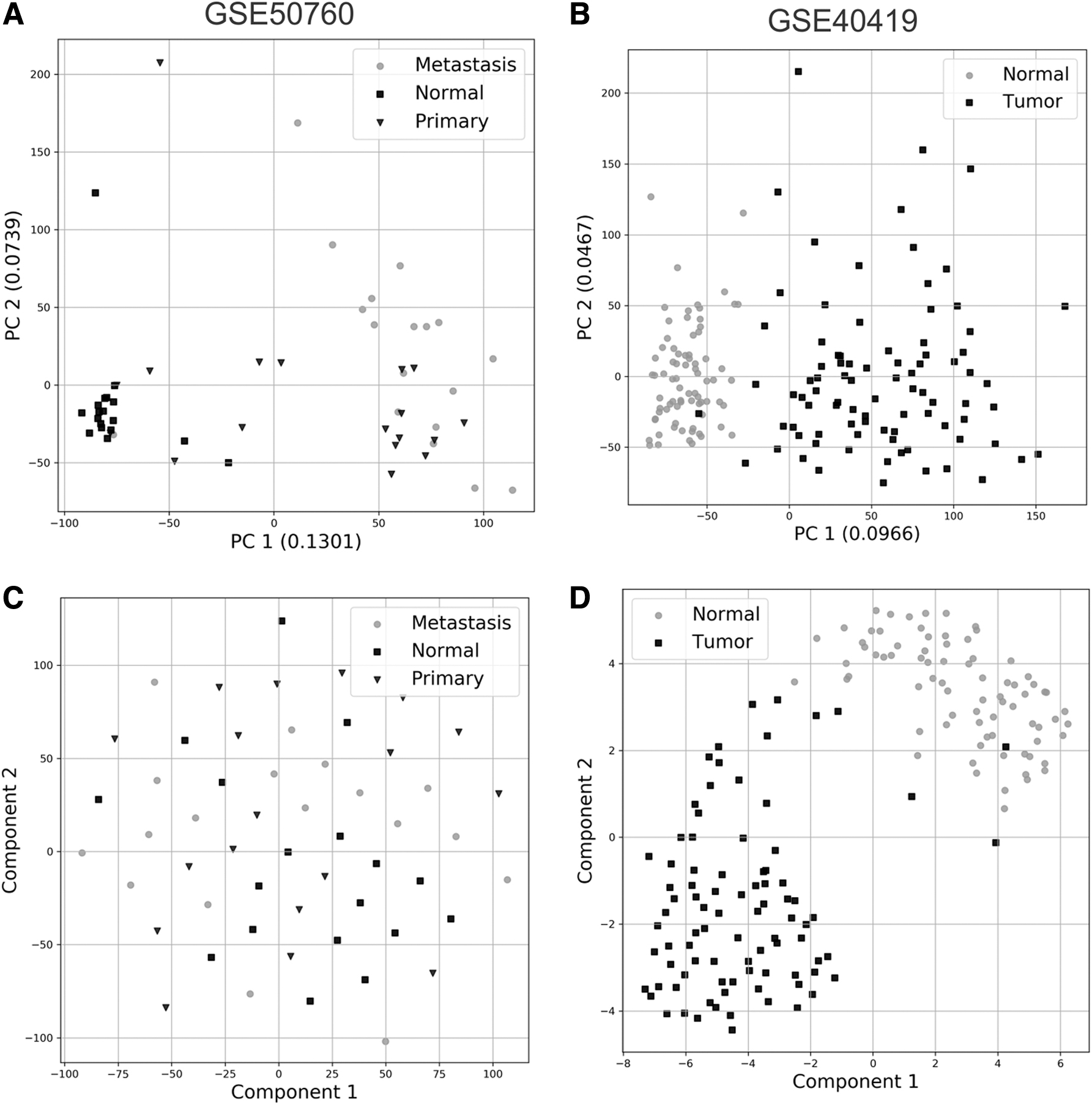
PCA and t-SNE plots for GSE50760 and GSE40419. These data sets were chosen as an example nonbinary (GSE50760) and binary (GSE40419) data sets currently available in BARRA:CuRDa. (A) PCA for GSE50760; (B) PCA for GSE40419; (C) t-SNE for GSE50760; (D) t-SNE for GSE40419. PCA and t-SNE results are available for all data sets in the database. GSE, Geo Series.

This lack of grouping observed for both analyses is a typical result when analyzing cancer data sets. Cancer is a heterogeneous disease by nature, differing even among similar subtypes (Archer et al., 2016). Thus, it is relatively common to see experimental (tumoral) samples being grouped closely to normal (healthy) samples in cancer studies because different tumoral cell populations might still possess similar molecular signatures to the adjacent healthy tissue. As an unsupervised technique, PCA globally analyzes data sets, with no class distinguishing, and separates the data based on each principal component's highest variance. It considers a linear correlation between features; thus, data inherited biased, such as tumoral samples, impose a technical difficulty for PCA, which is further increased by unbalanced data sets. Standardizing the initial input, like we did in both data gathering and preprocessing steps, is one way to increase PCA accuracy.

In contrast, t-SNE displayed worse results than PCA. One possible explanation is that t-SNE is a nondeterministic approach, and multiple runs could provide different results. Similarly, t-SNE is prone to the tuning of hyperparameters, which might influence final results.

Exceptions include GSE40419, which showed the best results in both analyses (Fig. 2B, D), and GSE69240, which displayed a better distribution on PCA analysis but not in t-SNE.

BARRA:CuRDa aims to provide basic comparisons using standard approaches so that researchers can devise better strategies for their algorithms. Hence, it is expected that any algorithms employing our data sets might achieve better PCA and t-SNE results than shown in this study.

3.2.2. Benchmarks

Generally, there was slight variation between the results when comparing the three experiments performed: (1) using all attributes without performing hyperparameter optimization; (2) using all attributes with the hyperparameter optimization; and (3) using the top 10 attributes and hyperparameter optimization (Supplementary Data). However, for some data sets with few samples, such as GSE48850, GSE55758, GSE63511, GSE64912, and GSE89122, we can see that utilizing the top 10 features to improve accuracy and reduce the possibility of overfitting resulted in slightly better results.

When considering three key indexes (F1-score, sensitivity, and specificity), we can discern that the FS technique improved the learning models regarding the classification of the original data. Nevertheless, GSE50760 and SRR2089755, the only nonbinary data sets, we see the opposite; the experiment employing the top 10 features displayed worse results. One possible explanation is that using only 10 features might not have been enough to create a robust predictive model that can separate samples in more complex class space. This result reflects the heat maps of these data sets (Supplementary Data). Thus, the results generated in this study further supports the employment of these metrics to analyze similar data sets. In addition, using the top 10 features to improve accuracy and avoid overfitting appears to be a valid approach, especially in data sets with fewer samples. It also enables making more precise correlations with biological results.

The heterogeneous results are likely reflections of the proportion between the low and unbalanced number of samples and the number of features of the gathered RNA-seq data sets. Unlike microarrays, in which the number of probes could be lower depending on the platform, results derived from RNA-seq will always have a large number of features, which imposes an extra layer of complexity to apply new ML approaches. In addition, some ML algorithms do not handle well with a skewed distribution of classes and generate incorrect predictive models. We can modify the training algorithm to work around this problem; this can be achieved by giving different weights to both majority and minority classes. The difference in weights will influence the classification of the classes during the training phase. The goal is to penalize the misclassification made by the minority class by setting a higher class weight while reducing the weight of the majority class. Another possibility is to use resampling techniques to balance classes.

The Synthetic Minority Oversampling TEchnique (SMOTE; Chawla et al., 2002) is an oversampling approach that creates synthetic minority class samples. To balance the minority class in the data set, SMOTE first selects a minority class data instance M_a randomly. Then, the k-NN of M_a, regarding the minority class, are identified. A second data instance M_b is then selected from the k-NN set. In this way, M_a and M_b are connected, forming a line segment in the feature space. The new synthetic data are then generated as a convex combination between M_a and M_b. This procedure occurs until the data set is balanced between the minority and majority classes. We performed two experiments for each data set with Shannon entropy <1.0 (Supplementary Data): (1) we applied the class weight technique for the DT, SVM, LR, and RF classifiers using the classweight sklearn parameter; and (2) we applied the SMOTE resampling technique and evaluated all classifiers. We observed that the application of both approaches equalizes the sensitivity and specificity values achieved by the classifiers, eliminating possible distortions caused by unbalanced data sets.

It is important to emphasize that, in most cases, the accuracy of the rating to measure the performance of the model is not enough to judge the model (Tharwat, 2020). We can have satisfactory results when evaluated using an accuracy metric. We can still have poor outcomes when assessed against other metrics, such as Logarithmic Loss, F1-score, or other metrics. In BARRA:CuRDa, most classes are unbalanced, which strongly limits the sole employment of accuracy. Future studies should employ more metrics to assess the precision of their algorithms. Hence, BARRA:CuRDa provides four additional benchmarks metrics that can be directly accessed through the database by clicking on the accuracy values.

3.2.3. Feature selection

In the world of Big Data and Data Science, data sample size and the number of characteristics are continuously growing (Bolón-Canedo et al., 2016; Li and Liu, 2017). FS has become an important research area in recent years because of the need to treat this massive amount of available information. The challenge consists of eliminating variables considered irrelevant in data sets (Jirapech-Umpai and Aitken, 2005). In some domains, as seen in Bioinformatics, especially in cancer research, the instances are described by dozens of thousands of features. The inclusion of irrelevant features increases the computational cost of the model's induction and prediction, impairs inference capacity, and high dimensions can reduce the capacity of ML techniques to generalize (Lazar et al., 2012; Aggarwal et al., 2014). Besides, FS also benefits data visualization and analysis of specific variants, helping to understand the research problem's core aspects.

BARRA:CuRDa brings additional FS tests that were absent in CuMiDa (Supplementary Data). The first reason to perform such analysis was to test each data set for its top features and validate their quality. It is expected that in a “prime” data set, the selection of meaningful features would be easier. The second reason was to provide a base FS for other approaches to compare their results. It is expected that new algorithms would extract significant features in terms of biological relevance, much like we exhibit in this study.

In this sense, we selected the top 10 features to observe how accurate the selection was for the biological background, which is cancer. The first aspect we noticed is that 12/17 data sets presented lncRNAs among their selected features, a total of 25 identified lncRNAs. This is an intriguing observation that could reflect the nature of FS approaches: to extract the features that best distinguish each class. LncRNAs are RNA molecules that are not coded for proteins; instead, they act as regulators of gene expression (Chan and Tay, 2018). Their detection is increasingly becoming crucial for cancer biology as lncRNAs are arising as significant drivers of the tumoral process in multiple cancer types (Niknafs et al., 2016; Song et al., 2017; Chan and Tay, 2018; Lingadahalli et al., 2018; Chi et al., 2019). In this sense, two lncRNA, AFAP1 antisense RNA1 (AFAP1-AS1) and cystatin-SN (CST1), appeared in more than two data sets. AFAP1-AS1 was present in three of the four lung data sets and is already described to promote migration, invasion, and proliferation of non-small cell lung carcinoma (Tang et al., 2018; Yin et al., 2018). In contrast, CST1, which was present in four data sets, including the three lung data sets earlier and one from breast cancer, was previously described to promote metastasis and increase poor prognosis in both lung and breast cancers (Cao et al., 2015; Dai et al., 2017). The fact that ML approaches can promptly identify lncRNA supports its use in the analysis of biological data (Fig. 3).

FIG. 3.

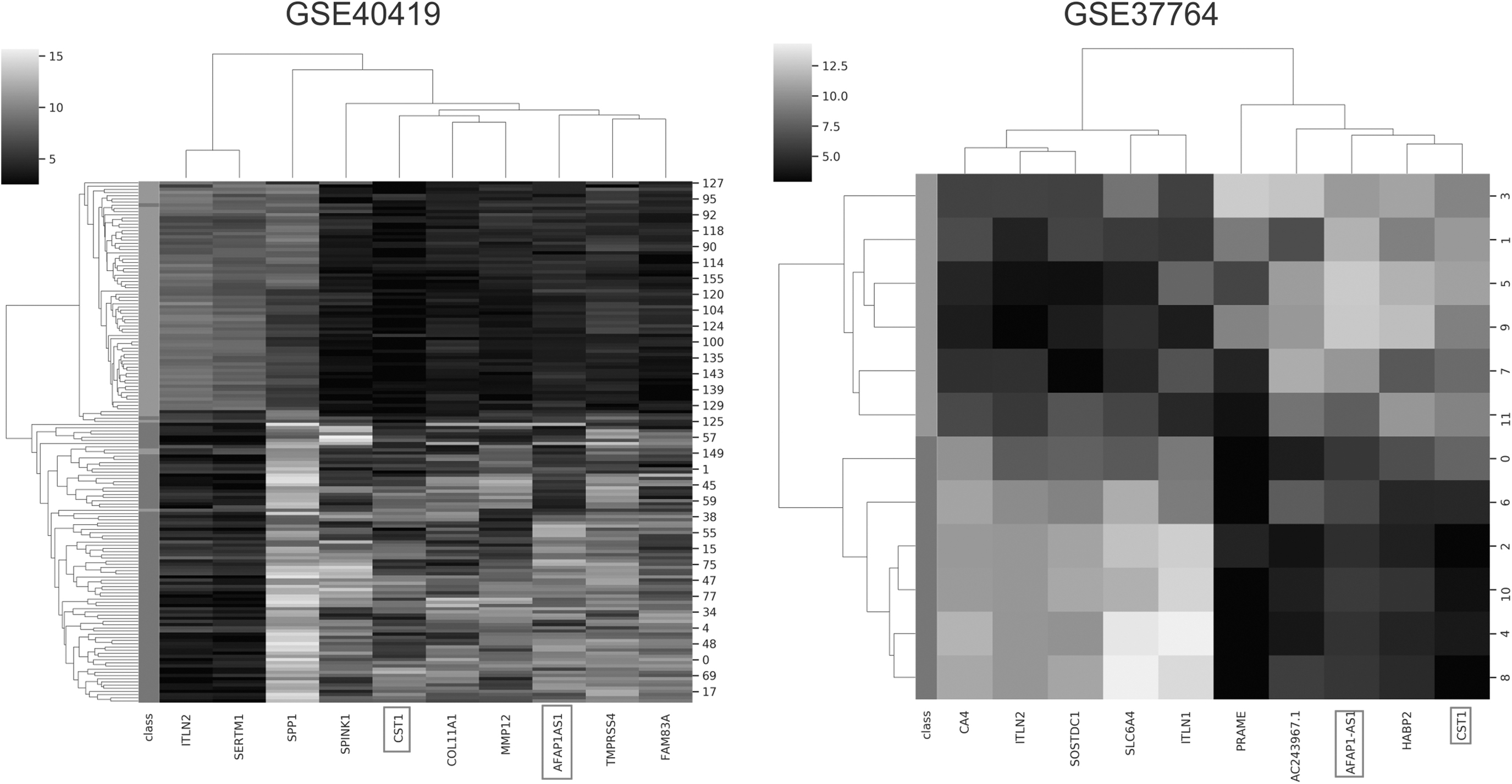
Heat maps of the top 10 features of GSE37764 and GSE40419. These lung cancer data sets were chosen as an example because they all showed AFAP1-AS1 (AFAP1 antisense RNA1) and CST1 (cystatin-SN) among their top features (dark squares). These heat maps are available for all data sets in the database.

Moreover, the FS method selected two pseudogenes in lung and head/neck cancer data sets (Supplementary Data). From both FS and biological points of view, this is an exciting result. Pseudogenes are gene copies that lost their original function, and despite the previous observation that declared them molecules with no biological function, new studies are showing that they have regulatory roles in both healthy and tumoral tissues (Tutar et al., 2016, 2018; De Martino et al., 2016; Chan and Tay, 2018; Kovalenko and Patrushev, 2018; Liu et al., 2019a). This is also in agreement with a recent ML study that reported the identification of four potential prognostic pseudogenes markers from osteosarcoma RNA-seq data (Liu et al., 2019b). Hence, FS methods could greatly aid in their identification, finding new targets that have relevant roles in cancer.

Finally, multiple other relevant genes linked to their specific tumoral process were selected by the basic FS method applied in this study, such as TDRD1 (Xiao et al., 2016), FOSL1 (Franco et al., 2018), CYP1A1 (Rodriguez and Potter, 2013), NXPH1 (Faryna et al., 2012), ORM2 (Zhang et al., 2012), FAM3B (Li et al., 2013), APOA1 (Aguirre-Portolés et al., 2018), XIST (Sun et al., 2019), FCN2 (Yang et al., 2016), HABP2 (Mirzapoiazova et al., 2015), SPINK1 (Xu et al., 2018), SLC34A2 (Jiang et al., 2016), LIPH (Ishimine et al., 2016), TCL1B (Rodríguez-Rodero et al., 2013), and ZCCHC12 (Wang et al., 2017), just to name a few. However, many other genes present in our list are already described to be part of the tumoral process but discussing all of them would be outside the scope of this study. Hence, new algorithms must be able to select relevant features, not necessarily matching those identified in this study, but at least in the same context of cancer.

4. CONCLUSION AND PERSPECTIVES

ML algorithms are gradually gaining more attention from biomedical sciences; their applications are becoming broader and progressively more accurate as we devise rigorous methods. However, this is directly linked to data availability, which allows the training and testing of new algorithms. In this pursuit of more modern and increasingly precise approaches, databases that bring up-to-date, curated, and preprocessed data using state-of-the-art protocols are of extreme importance since training and testing such algorithms with reliable data unequivocally create more realistic results. BARRA:CuRDa will be an essential asset in validating new approaches and testing new ML algorithms focused on analyzing biomedical data for cancer research. In addition, it can be an important tool for comparing ML strategies with different types of data.

Both CuMiDa and BARRA:CuRDa will soon receive massive updates. Future perspectives will include more organisms and newer metrics for benchmarking, a new R package, and Python scripts for direct download.

Footnotes

AUTHOR DISCLOSURE STATEMENT

The authors declare they have no competing financial interests.

FUNDING INFORMATION

This study was supported by grants from the Fundação de Amparo à Pesquisa do Estado do Rio Grande do Sul—FAPERGS (19/2551-0001906-8), Conselho Nacional de Desenvolvimento Científico e Tecnológico—CNPq (311611/2018-4), and the Coordenação de Aperfeiçoamento de Pessoal de Nível Superior—STICAMSUD (88881.522073/2020-01)—Brazil. This study was financed in part by the Coordenação de Aperfeiçoamento de Pessoal de Nível Superior—Brasil (CAPES)—Finance Code 001.

SUPPLEMENTARY MATERIAL

References

Aguirre-Portolés

, Feliu

, Reglero

, et al. 2018. Abca1 overexpression worsens colorectal cancer prognosis by facilitating tumour growth and caveolin-1-dependent invasiveness, and these effects can be ameliorated using the bet inhibitor apabetalone. Mol. Oncolgy. 12, 1735–1752.

Archer

T.C.

, Fertig

E.J.

, Gosline

S.J.

, et al. 2016. Systems approaches to cancer biology. Cancer Res. 76, 6774–6777.

Blalock

E.M.

2003. A Beginner's Guide to Microarrays. Springer: Boston, Massachusetts, USA.

Blohm

and Guiseppi-Elie

2001. New developments in microarray technology. Curr. Opin. Biotechnol. 12, 41–47.

Bolger

A.M.

, Lohse

, and Usadel

2014. Trimmomatic: A flexible trimmer for illumina sequence data. Bioinformatics. 30, 2114–2120.

Bolón-Canedo

, Sánchez-Maroño

, and Alonso-Betanzos

2016. Feature selection for high-dimensional data. Progr. Artif. Intell. 5, 65–75.

Breiman

2001. Random forests. Mach. Learn. 45, 5–32.

Cao

, Li

, Luo

R.-Z.

, et al. 2015. Expression of cystatin sn significantly correlates with recurrence, metastasis, and survival duration in surgically resected non-small cell lung cancer patients. Sci. Rep. 5, 8230.

Cerami

, Gao

, Dogrusoz

, et al. 2012. The cbio cancer genomics portal: An open platform for exploring multidimensional cancer genomics data. Cancer Discov. 2, 401–404.

10.

Chan

J.J.

and Tay

2018. Noncoding RNA: RNA regulatory networks in cancer. Int. J. Mol. Sci. 19, 1310.

11.

Chawla

N.V.

, Bowyer

K.W.

, Hall

L.O.

, et al. 2002. Smote: Synthetic minority over-sampling technique. J. Artif. Int. Res. 16, 321–357.

12.

Chi

, Wang

, et al. 2019. Long non-coding RNA in the pathogenesis of cancers. Cells. 8, 1015.

13.

Cortes

and Vapnik

1995. Support-vector networks. Mach. Learn. 20, 273–297.

14.

Dai

.-n., Li

, Chen

, et al. 2017. Elevated expression of cst1 promotes breast cancer progression and predicts a poor prognosis. J. Mol. Med. 95, 873–886.

15.

Davis

and Meltzer

2007. Geoquery: A bridge between the gene expression omnibus (GEO) and bioconductor. Bioinformatics. 14, 1846–1847.

16.

De Martino

, Forzati

, Arra

, et al. 2016. Hmga1-pseudogenes and cancer. Oncotarget. 7, 28724.

17.

Dobin

, Davis

C.A.

, Schlesinger

, et al. 2013. STAR: Ultrafast universal RNA-seq aligner. Bioinformatics. 29, 15–21.

18.

Epstein

and Butow

2000. Microarray technology—enhanced versatility, persistent challenge. Curr. Opin. Biotechnol. 11, 36–41.

19.

Faryna

, Konermann

, Aulmann

, et al. 2012. Genome-wide methylation screen in low-grade breast cancer identifies novel epigenetically altered genes as potential biomarkers for tumor diagnosis. FASEB J. 26, 4937–4950.

20.

Feltes

B.C.

, Chandelier

E.B.

, Grisci

B.I.

, et al. 2019. Cumida: An extensively curated microarray database for benchmarking and testing of machine learning approaches in cancer research. J. Comput. Biol. 26, 376–386.

21.

Franco

H.L.

, Nagari

, Malladi

V.S.

, et al. 2018. Enhancer transcription reveals subtype-specific gene expression programs controlling breast cancer pathogenesis. Genome Res. 28, 159–170.

22.

Frank

, Hall

M.A.

, and Witten

I.H.

2016. The WEKA Workbench. Online Appendix for “Data Mining: Practical Machine Learning Tools and Techniques.” Morgan Kaufmann, 4th edition.

23.

Geisser

1975. The predictive sample reuse method with applications. J. Am. Stat. Assoc. 70, 320–328.

24.

Geraci

, Saha

, and Bianchini

2020. Rna-seq analysis: Methods, applications and challenges. Front. Genet. 11, 220.

25.

Harrington

2012. Machine Learning in Action, Volume 5. Manning Greenwich, CT, Shelter Island, NY, 11964.

26.

Hrdlickova

, Toloue

, and Tian

2017. Rna-seq methods for transcriptome analysis. Wiley Interdiscipl. Rev. RNA. 8, e1364.

27.

Huang

. and Li

. 2011. Naive Bayes classification algorithm based on small sample set, 34–39. CCIS2011-Proceedings: 2011 IEEE International Conference on Cloud Computing and Intelligence Systems, Beijing, China.

28.

Ishimine

, Zhou

, Sumitomo

, et al. 2016. Lipase member h frequently overexpressed in human esophageal adenocarcinomas. Tumor Biol. 37, 2075–2081.

29.

Jiang

, Hao

, Ding

, et al. 2016. The effects and mechanisms of slc34a2 on tumorigenicity in human non-small cell lung cancer stem cells. Tumor Biol. 37, 10383–10392.

30.

Jirapech-Umpai

and Aitken

2005. Feature selection and classification for microarray data analysis: Evolutionary methods for identifying predictive genes. BMC Bioinform. 6, 148.

31.

Kotsiantis

S.B.

, Zaharakis

I.D.

, and Pintelas

P.E.

2006. Machine learning: A review of classification and combining techniques. Artif. Intell. Rev. 26, 159–190.

32.

Kovalenko

and Patrushev

2018. Pseudogenes as functionally significant elements of the genome. Biochemistry (Moscow). 83, 1332–1349.

33.

Kubat

2017. An Introduction to Machine Learning. Springer International: Switzerland, 1st edition.

34.

Lachenbruch

P.A.

and Mickey

M.R.

1968. Estimation of error rates in discriminant analysis. Technometrics. 10, 1–11.

35.

Lazar

, Taminau

, Meganck

, et al. 2012. A survey on filter techniques for feature selection in gene expression microarray analysis. IEEE ACM Trans. Comput. Biol. Bioinform. 9, 1106–1119.

36.

and Dewey

C.N.

2011. RSEM: Accurate transcript quantification from RNA-seq data with or without a reference genome. BMC Bioinfo. 12, 323.

37.

and Liu

2017. Challenges of feature selection for big data analytics. IEEE Intell. Syst. 32, 9–15.

38.

W.V.

and Li

J.J.

2018. Modeling and analysis of RNA-seq data: A review from a statistical perspective. Quant. Biol. 6, 195–209.

39.

, Mou

, Wang

, et al. 2013. A non-secretory form of fam3b promotes invasion and metastasis of human colon cancer cells by upregulating slug expression. Cancer Lett. 328, 278–284.

40.

Lingadahalli

, Jadhao

, Sung

Y.Y.

, et al. 2018. Novel lncRNA LINC00844 regulates prostate cancer cell migration and invasion through AR signaling. Mol. Cancer Res. 16, 1865–1878.

41.

Liu

, Liu

, et al. 2019a. A prognostic signature of five pseudogenes for predicting lower-grade gliomas. Biomed. Pharmacother. 117, 109116.

42.

Liu

, Xing

, Zhang

, et al. 2019b. A four-pseudogene classifier identified by machine learning serves as a novel prognostic marker for survival of osteosarcoma. Genes. 10, 414.

43.

Love

M.I.

, Huber

, and Anders

2014. Moderated estimation of fold change and dispersion for RNA-seq data with deseq2. Genome Biol. 15, 550.

44.

Maaten

.v.d. and Hinton

. 2008. Visualizing data using t-SNE. J. Mach. Learn Res. 9, 2579–2605.

45.

Mirzapoiazova

, Mambetsariev

, Lennon

F.E.

, et al. 2015. Habp2 is a novel regulator of hyaluronan-mediated human lung cancer progression. Front. Oncol. 5, 164.

46.

Niknafs

Y.S.

, Han

, Ma

, et al. 2016. The lncRNA landscape of breast cancer reveals a role for DSCAM-AS1 in breast cancer progression. Nat. Commun. 7, 1–13.

47.

Pedregosa

, Varoquaux

, Gramfort

, et al. 2011. SCIKIT-learn: Machine learning in python. J. Mach. Learn. Res. 12, 2825–2830.

48.

Rodriguez

and Potter

D.A.

2013. Cyp1a1 regulates breast cancer proliferation and survival. Mol. Cancer Res. 11, 780–792.

49.

Rodríguez-Rodero

, Fernández

A.F.

, Fernández-Morera

J.L.

, et al. 2013. DNA methylation signatures identify biologically distinct thyroid cancer subtypes. J. Clin. Endocrinol. Metabol. 98, 2811–2821.

50.

Safavian

S.R.

and Landgrebe

1991. A survey of decision tree classifier methodology. IEEE Trans. Syst. Man Cybernet. 21, 660–674.

51.

Šimundić

A.-M.

2009. Measures of diagnostic accuracy: Basic definitions. Ejifcc. 19, 203.

52.

Sokolova

, Japkowicz

, and Szpakowicz

2006. Beyond accuracy, f-score and ROC: A family of discriminant measures for performance evaluation, 1015–1021. In Sattar, A., and Kang, B., eds. AI 2006: Advances in Artificial Intelligence. Springer, Berlin, Heidelberg.

53.

Soneson

, Love

M.I.

, and Robinson

M.D.

2015. Differential analyses for RNA-seq: Transcript-level estimates improve gene-level inferences. F1000Res. 4, 1521.

54.

Song

, Jiang

, Liu

, et al. 2017. A three-lncRNA expression signature associated with the prognosis of gastric cancer patients. Cancer Med. 6, 1154–1164.

55.

STONE

1977. Asymptotics for and against cross-validation. Biometrika. 64, 29–35.

56.

Sun

, Jia

, Duan

, et al. 2019. Long non-coding RNA XIST regulates mir-106b-5p/p21 axis to suppress tumor progression in renal cell carcinoma. Biochem. Biophys. Res. Commun. 510, 416–420.

57.

Tang

, Alelyani

, and Liu

2014. Feature selection for classification: A review. In Aggarwal, C.C. ed. Data Classification: Algorithms and Applications. (first edition). Chapman and Hall/CRC. Pgs 37–58.

58.

Tang

X.-D.

, Zhang

D.-D.

, Jia

, et al. 2018. lncRNA AFAP1-AS1 promotes migration and invasion of non-small cell lung cancer via up-regulating IRF7 and the rig-i-like receptor signaling pathway. Cell. Physiol. Biochem. 50179–195.

59.

Tharwat

2020. Classification assessment methods. Appl. Comput. Inform. 17, 168–192.

60.

Tutar

, Özgür

, and Tutar

2018. Involvement of miRNAs and pseudogenes in cancer, 45–66. In Wu, W. ed. MicroRNA and Cancer. Methods in Molecular Biology, vol 1699. Humana Press: New York, New York, USA.

61.

Tutar

, Özgür

, Tutar

, et al. 2016. Regulation of oncogenic genes by micrornas and pseudogenes in human lung cancer. Biomed. Pharmacother. 83, 1182–1190.

62.

Van Den Berge

, Hembach

K.M.

, Soneson

, et al. 2019. RNA sequencing data: Hitchhiker's guide to expression analysis. Ann. Rev. Biomed. Data Sci. 2, 139–173.

63.

Verleysen

and François

2005. The curse of dimensionality in data mining and time series prediction. IWANN. 5, 758–770.

64.

Wang

, Zheng

, Wang

, et al. 2017. Zcchc12, a novel oncogene in papillary thyroid cancer. J. Cancer Res. Clin. Oncol. 143, 1679–1686.

65.

Xiao

, Lanz

R.B.

, Frolov

, et al. 2016. The germ cell gene TDRD1 as an erg target gene and a novel prostate cancer biomarker. Prostate. 76, 1271–1284.

66.

, Lu

, Huang

, et al. 2018. SPINK1 promotes cell growth and metastasis of lung adenocarcinoma and acts as a novel prognostic biomarker. BMB Reports. 51, 648.

67.

Yang

, Liang

, Zheng

, et al. 2016. FCN2 inhibits epithelial–mesenchymal transition-induced metastasis of hepatocellular carcinoma via TGF-β/SMAD signaling. Cancer Lett. 378, 80–86.

68.

Yin

, Lu

, Su

, et al. 2018. Long noncoding RNA AFAP1-AS1 predicts a poor prognosis and regulates non–small cell lung cancer cell proliferation by epigenetically repressing p21 expression. Mol. Cancer. 17, 1–12.

69.

Zararsız

2015. Development and application of novel machine learning approaches for RNA-seq data classification. Int. J. Comput. Trends Tech. (IJCT). 2017, 62–64.

70.

Zhang

, Xiao

, Liu

, et al. 2012. The potential role of ORM2 in the development of colorectal cancer. PLoS One. 7, e31868.

Supplementary Material

Please find the following supplemental material available below.

For Open Access articles published under a Creative Commons License, all supplemental material carries the same license as the article it is associated with.

For non-Open Access articles published, all supplemental material carries a non-exclusive license, and permission requests for re-use of supplemental material or any part of supplemental material shall be sent directly to the copyright owner as specified in the copyright notice associated with the article.

0.00 MB

4.73 MB