Calculating Orthologous Protein-Coding Sequence Set Probability Using the Poisson Process

Abstract

We extend the popular Jukes–Cantor evolution model and calculate the probability of an orthologous nucleotide sequence set [a reference sequence (B₁) stays with the other sequences (B₋₁)], where the sequence evolution [from a last common ancestral sequence (ɑ)] follows the (prospective) Poisson process with the overall event rate λ prorated among mutation types (nucleotide/codon substitution, insertion, and deletion) and sites along each sequence. The corresponding retrospective process (reversing the prospective process) facilitates developing algorithms to calculate the marginal probability [Pr(B₁)] (Monte Carlo integration) and sample ɑ (given B₁). We calculate probability Pr(B₋₁|ɑ) based on the identified events (during “ɑ→B₋₁”) from pairwise sequence alignment to implement Pr(B₋₁|B₁) calculation (Monte Carlo integration). Event queue sampling and probability magnifiers are used to improve the computational efficiency when the number of events is large. We finally test our procedure on both simulated and recently studied hexapod transcriptome data (Brandt et al.), where each asexual lineage pairs with its closest related sexual lineage. Rate estimates (for Phasmatodea and Zygentoma) and model comparison indicate that the asexual lineages likely mutate several times faster than their sexual relatives.

1. Introduction

As interdisciplinary research in molecular evolution continuously grows, many statistical models and computation procedures have been developed for making rigorous inference out of the phylogeny analysis. Among them, robust methods (represented by maximum likelihood estimation [MLE]) against model violations are particularly popular with tree likelihood (probability) as an optimization criterion. Thorne et al. (1991) presented a remarkable MLE framework (TKF91 model) for evolutionary models involving single-base substitution and indel (insertion, deletion) between two DNA sequences, where the likelihood involves summing over all possible alignments, the equilibrium ancestral sequence probability (to ensure the reversibility of the evolution process) and separate processes (for substitution and indel). MOLPHY (molecular phylogenetics based on maximum likelihood) (Adachi and Hasegawa, 1992) offers a number of specific models with algorithms to construct the evolutionary tree from orthologous mtDNA sequences with nucleotide and/or codon substitution. The considered components include the distance matrix, transition probability matrix, relative substitution rate, biased nucleotide composition, distinct transition and transversion rates, nucleotide dependence in a codon, fourfold degenerate sites of mitochondria, and others. Given tree topology, the relative substitution rates and branch lengths (numbers of nucleotide substitutions) are estimated possibly with the help of selected outgroup references.

Among many recent algorithms, BEAST (Suchard et al., 2018) performs Bayesian phylogeny tree sampling to do continuous phylogeographic analyses for fast-evolving avian influenza viruses, PhyML (Oliva et al., 2019) reconstructs the last common ancestor (LCA) sequence for the substitution model with multiple alignment involved, and MELTOS (Camir et al., 2020) uses somatic single nucleotide variants to construct the tumor phylogeny tree. Aside from these advancements, reformed MLE frameworks taking into account other realistic scenarios (e.g., large indels, multiple unaligned sequences) are still anticipated (Thorne et al., 1991).

In the sequel, notations “a” and “B” represent the unobserved LCA and the observed species-specific nucleotide sequence, respectively. The word “letter” represents a distinct nucleotide label (A, T, C, or G) per relevant literature. We use the star (parallel) evolution case (the left panel, Fig. 1) as an illustrative example where the joint probability of B_1:3 is of our interest. A naive way might be reporting it as the proportion of observing B_1:3 out of a number of simulated B_1:3 sets, where each set undergoes mutation from certain a drawn from certain population. However, the chance of observing a specific B_1:3 becomes negligible when ɑ follows a noninformative prior distribution (π(ɑ)) among the population. Liu et al. (2009) assumed that each nucleotide site separately follows an evolution model and proposed sampling ɑ (given a reference sequence B₁) and Monte Carlo integration of transition (ɑ→B_2:3) probabilities to compute Pr(B_1:3) as Pr(B₁) × Pr(B_2:3|B₁). Since each protein-coding locus (sequence) is likely a functional unit in a biological pathway, we presently take the whole sequence as the object and calculate Pr(B_1:3) within the framework of a self-contained continuous-time Poisson process, where a prospective process (M) is reverted by its retrospective process (M*).

FIG. 1.

Evolution scenarios (star and phylogeny tree). r, a, and B1:3 represent the root, the LCA and the observed species sequences, respectively. The divergence time (T) and the generic event rate (λ) from the preceding node to the current node are in the brackets. LCA, last common ancestor.

Compared with other approaches, our contributions include the following advantages. We involve less model parameters by appropriately prorating the overall generic event rate (λ) among detailed events (e.g., site-and-letter-specific substitutions and indels of nucleotide and codon) based on specified prorate weights. The resultant constant detailed-event ratio (between M and M*) leads to efficient sampling (for a) and sequence set probability calculation. We do not need multiple alignment, an outgroup reference sequence, the reversibility condition, or an informative prior distribution (for a), among others. The working sequence lengths are realistic (up to 10³). We test our algorithm on both simulated and real-world protein-coding loci data. Our numerical results show that maximizing the probability of the observed species sequence set enables quantifying distinct evolution rates along different lineages.

This article is organized as follows. Section 2 illustrates the Poisson process where events during the prospective process match the retrospective events (with a constant rate ratio); the probability of sequence mutation (from ɑ to any observed sequence B) is derived under realistic scenarios (e.g., involving nucleotide and/or codon indels); and algorithms are introduced for calculating Pr(B_1:3) through computing Pr(B₁) and sampling ɑ (given B₁). Section 3 tests our method on both artificial data and a family of real orthologous protein-coding sequences from a recent study. Section 4 concludes with discussion and some future directions.

2. Methods

2.1. Prospective and retrospective sequence mutation processes

The popular Jukes–Cantor (JC) model (Jukes and Cantor, 1969) assumes a constant overall mutation rate (λ) and equal weights among four letters at nucleotide substitution. The instants of our generic events [substitution (S), insertion (I), and deletion (D)] (during mutation ɑ→B) follow a continuous-time Poisson process with up to one event occurrence at any instant. Such a prospective process (denoted by M) is described as follows (the upper panel, Table 1). We introduce N_n: = {1,…,n} and Z_n: = {0,…,n − 1}. Let t_B be the terminal instant and n be the number of events during $(0, t_{B}] = {(t_{i - 1}, t_{i}), i \in N_{n}} \cup {t_{i}, i \in N_{n}} \cup (t_{n}, t_{B}]$ . Here, no events occur within each open or half-open time segment $({(t_{i - 1}, t_{i}), i \in N_{n}}, (t_{n}, t_{B}])$ and one single event occurs at each instant ${t_{i}, i \in N_{n}}$ . The event (at t_i) is denoted as $e_{i} (i \in N_{n})$ , which is S, I, or D.

Table 1.

The Illustration of the Poisson Process

The prospective process (a→B)
Instant	$t_{0} = : 0$	→	{t₁}	→	{t₂}	…	{ $t_{n - 1}$ }	→	{t_n}	→	t_B
Event			e ₁		e ₂	…	$e_{n - 1}$		e_n
State	x ₀		x₀ → x₁		x₁ → x₂	…	$x_{n - 2}$ → $x_{n - 1}$		$x_{n - 1}$ → x_n
Length	l ₀		l₀ → l₁		l₁ → l₂	…	$l_{n - 2}$ → $l_{n - 1}$		$l_{n - 1}$ → l_n
The retrospective process (a←B)

The temporal evolution events, sequence states, and lengths on the retrospective process (M^*) reverse those corresponding events, states, and lengths on the prospective process (M) at matched instants. a and B represent the ancestor and the evolved observed sequence, respectively.

The complete information includes the transient sequence states $x_{i} (i \in {Z_{n}}_{+ 1})$ (during mutation from a to the terminal state B) and event instants $t_{i} (i \in {Z_{n}}_{+ 1})$ . The state is x₀ during time period (t₀ = 0, t₁) and mutates (x₀→x₁) at t₁ with length change (l₀→l₁). The state remains as x₁ during (t₁, t₂) and mutates (x₁→x₂) at t₂ with length change (l₁→l₂). Finally, the state stays as x_n during period (t_n,t_B) and mutation (a→B) completes at t_B. M matches a retrospective process (M*), which takes sequence B as the “initial” state and traces back to ɑ (with t₀* and t_B* as the “starting” and “ending” time points). For $i \in N_{n}$ , event e_i* (x_i₋₁*→x_i*) at t_i* (on M*) reverses e_n _{+ 1−i} (x_n_−i→x_n _{+ 1−i}) at t_n _{+ 1−i} (on M) and length change l_i₋₁*→l_i* reverses l_n_−i→l_n _{+ 1−i}. We assume a constant generic event rate (λ(t) = λ) on M and let $(λ_{0, S}^{}, λ_{0, I}^{}, λ_{0, D}^{})$ represent the prorated event-type-specific rates (among {S, I, D}), which are defined as: $(λ_{0, S}, λ_{0, I}, λ_{0, D}) = (p_{S}, p_{I}, p_{D}) λ .$

Here, the prorate weights satisfy $p_{S} + p_{I} + p_{D} = 1$ and subscript “0” represents the initial level of hierarchical prorating (among event types). We further consider l + 1 links along the current sequence with l nucleotides. For example, a four-nucleotide-long sequence “ATCG” (subject to modeling) with five links can be written as “-A-T-C-G-,” where each “-” represents a link and two ending links (the leftmost and rightmost) may be connected to other irrelevant nucleotides (not involved in the Poisson process) along the genome. A new nucleotide (X∈{A,T,C,G}) insertion may take place as -A-X-T-C-G- (at the second link) or -A-T-C-G-X- (at the fifth link) with equal chance (not specific to letters or link locations). This simple assumption does not distinguish between the normal and immortal links (TKF91 model) and streamlines our modeling and computation procedures. Thus, when the current sequence has l nucleotides, the prorated site-letter-specific event rates ( $λ_{1, S}^{}, λ_{1, I}^{}, λ_{1, D}^{}$ ) are defined as $(λ_{1, S}, λ_{1, I}, λ_{1, D}) = (\frac{p_{S}}{3 l}, \frac{p_{I}}{4 (l + 1)}, \frac{p_{D}}{l}) λ .$

Here, subscript “1” represents the next level of hierarchical prorating [involving four letters (A,T,C,G) and those sites along the nucleotide sequence]. This definition is sequence-length (l)-specific. Here, p_S/(3l) represents the prorate among three letters (possible states mutated from the original letter) and l nucleotides (for a substitution), p_I/4(l + 1) represents the prorate among four letters and l + 1 links (for an insertion), and p_D/l represents the prorate among l nucleotides (for a deletion). When LCA is long enough (∼10³) and the evolution involves a small number of indels (relative to current sequence length), the denominator is non-zero and the definition is valid. Similarly, we denote S*, D*, and I* as the events (on M*) reverting to S, I, and D (on M). We let M* also have a generic event rate $λ$ with the prorated rates (among {S*,I*,D*}) to be $(λ_{0, S^{*}}, λ_{0, I^{*}}, λ_{0, D^{*}}) = (p_{S}^{*}, p_{I}^{*}, p_{D}^{*}) λ w i t h p_{S}^{*} + p_{I}^{*} + p_{D}^{*} = 1 .$

The prorated site-letter-specific event rates are $(λ_{1, S^{*}}, λ_{1, I^{*}}, λ_{1, D^{*}}) = (\frac{p_{S}^{*}}{3 l}, \frac{p_{I}^{*}}{4 (l + 1)}, \frac{p_{D}^{*}}{l}) λ .$

Matching M with M* (with a constant site-letter-specific rate ratio) requires $(\frac{p_{S}}{3}) : (\frac{p_{I}}{4}) : (\frac{p_{D}}{1}) = (\frac{p_{S}^{*}}{3}) : (\frac{p_{D}^{*}}{1}) : (\frac{p_{I}^{*}}{4})$ (1)

with normalized prorated rates among {S*,I*,D*} to be , where . The resultant site-letter-specific rate ratio (M:M*) is ω.

2.2. Sequence transition probability

2.2.1. Nucleotide substitution–insertion–deletion model

For calculating the mutation probability (P_M(ɑ→B)) (M represents the prospective process), we let t₁ <…<t_n be the n random event instants and t_B be a right-censoring time (t_n < t_B < t_n _{+ 1}, t_n _{+ 1} is the anticipated n + 1_th event instant). The settings in Section 2.1 and relevant theories on the Poisson process (e.g., Rigdon and Basu, 2000, p54) lead to the following joint probability density function for a queue of n event instants on (0, t_B] $f_{a B} (T_{1} = t_{1}, \dots, T_{n} = t_{n}, T_{n + 1} > t_{B}) = λ^{n} e^{- λ t_{B}} \prod_{i \in N_{n}} (\frac{p_{S} 1_{\{S\} i}}{3 l_{i - 1}}, \frac{p_{I} 1_{\{I\} i}}{4 (l_{i - 1} + 1)}, \frac{p_{D} 1_{\{D\} i}}{l_{i - 1}}) .$ (2)

Here, 1_{S}i,1_{I}i and 1_{D}i are indicators for S, I, and D, respectively. Since the generic event rate λ(t) is a constant, the probability density [Eq. (2)] does not explicitly involve the event instants. In the sequel, f_aB(t_1:n,B) stands for the left-hand side of Eq. (2). Figure 2 shows an example with n = 6 (two substitutions, two insertions, and two deletions).

FIG. 2.

Six mutation events jointly cause “a→B.”

We let $ẽ : = (e_{1}, \dots, e_{n})$ be a specific queue of n [denoted as n(ɑ,B)] events and E_n be the set of all feasible queues, that is, is a queue of n events such that ɑ evolves into B}. The mutation (ɑ→B) probability [conditional on n(ɑ,B)] is

Here, we integrate f_aB(t_1:n,B) over the n-dimensional simplex {0 ≤ t₁ < $\dots$ < t_n ≤ t_B}, which has a volume of V(n, t_B) = t_Bⁿ/n!. Plugging Eq. (2) into Eq. (3) leads to ${P r}_{M} (a \to B |n (a, B)) = \frac{1}{n!} exp (- λ t_{B}) {(λ t_{B}^{})}^{n} \sum_{ẽ \in E_{n}} [\prod_{i \in N_{n}} (\frac{p_{S} 1_{\{S\} i}^{}}{3 l_{i - 1}^{}}, \frac{p_{I} 1_{\{I\} i}^{}}{4 (l_{i - 1}^{} + 1)}, \frac{p_{D} 1_{\{D\} i}^{}}{l_{i - 1}^{}})] .$ (4)

Similarly, we let $ẽ^{*} : = {e_{1}^{*}, \dots, e_{n}^{*}}$ be a queue of n matched events (on M*) and E_n* be the set of all such queues, that is, is a queue of n events such that B reverts to ɑ}. Given the number of events (n(B,ɑ) = n(ɑ,B)), the retrospective mutation probability [refer to Eqs. (2)–(4)] is ${P r}_{M} (B \to a |n (B, a)) = \frac{1}{n!} exp (- λ t_{B}) {(λ t_{B})}^{n} \sum_{ẽ^{*} \in E_{n}^{*}} [\prod_{i \in N_{n}} (\frac{p_{S}^{*} 1_{\{S\} i}^{*}}{3 l_{i - 1}^{*}}, \frac{p_{I}^{*} 1_{\{I\} i}^{*}}{4 l_{i - 1}^{*}}, \frac{p_{D}^{*} 1_{\{D\} i}^{*}}{l_{i - 1}^{*} + 1})] .$ (5)

Here, $1_{{S} i}^{*} = 1_{{S} n - i + 1},_{} 1_{{I} i}^{*} = 1_{{D} n - i + 1}$ and $1_{{D} i}^{*} = 1_{{I} n - i + 1} .$ The constant site-letter-specific rate ratio (ω) [Eq. (1), Section 2.1] ensures that each pair of length-n products [in the brackets, Eqs. (4) and (5)] has a ratio of ωⁿ (M:M*) and the probabilities [Eqs. (4) and (5)] have a ratio $c (a, B, n) : = \frac{{Pr}_{M} (a \to B | n (a, B))}{{Pr}_{M^{*}} (B \to a | n (B, a))} = ω^{n} (f r e e o f λ) .$ (6)

2.2.2. Codon insertion and deletion

Protein-coding sequence may experience codon (a nucleotide triplet) insertion or deletion (denoted as Ic or Dc). A constant event-specific rate ratio (M:M*) requires $(\frac{p_{S}}{3}) : (\frac{p_{I}}{4}) : (\frac{p_{D}}{1}) : (\frac{p_{I c}}{64}) : (\frac{p_{D c}}{1}) = (\frac{p_{S}^{*}}{3}) : (\frac{p_{D}^{*}}{1}) : (\frac{p_{I}^{*}}{4}) : (\frac{p_{D c}^{*}}{1}) : (\frac{p_{I c}^{*}}{64}),$

that is, , where and 64 is the number of distinct nucleotide triplets. The enhanced version of Eq. (2) is $f_{a B} (t_{1 : n, B}) = λ^{n} e^{- λ t_{B}} \prod_{i \in N_{n}} (\frac{p_{S} 1_{\{S\} i}}{3 l_{i - 1}}, \frac{p_{I} 1_{\{I\} i}}{4 (l_{i - 1} + 1)}, \frac{p_{D} 1_{\{D\} i}}{l_{i - 1}}, \frac{p_{I c} 1_{\{I c\} i}}{64 (l_{i - 1} + 1)}, \frac{p_{D c} 1_{\{D c\} i}}{l_{i - 1} - 2}) .$

Here, 1_{S}i, 1_{I}i, 1_{D}i, 1_{Ic}i, and 1_{Dc}i are indicators for nucleotide S-I-D and codon I-D, respectively. Equations (2)–(6) undergo corresponding adjustments. When n is large, exhaustive enumeration for E_n [in Eq. (4)] is replaced by a sampled subset [with m (<n!) queues] subject to adjustment (probability multiplied by n!/m).

2.3. Calculate sequence set probability

We specify an informative [e.g., Eq. (8)] or noninformative [a special case of Eq. (8), Sections 3.1 and 3.2] prior distribution (π(a)) when the compositional information on a is available or not. The set probability in the star scenario is presented as $\begin{matrix} Pr (B_{1 : 3}) & = Pr (B_{2 : 3} | B_{1}) Pr (B_{1}) = [\sum_{a \in A} Pr (B_{2 : 3} | a) Pr (a | B_{1})] \times Pr (B_{1}) \\ = [\sum_{a \in A} Pr (B_{2} | a) Pr (B_{3} | a) Pr (a | B_{1})] \times [\sum_{a \in A} Pr (B_{1} | a) π (a)] . \end{matrix}$ (7)

Here, “A” (in the subscript of Σ) represents the ancestor sequence (a) population (not a letter for nucleotide “A”) and B₁ is the reference sequence used for sampling ɑ based on the posterior distribution $Pr (a |B_{1}) = \frac{Pr (a, B_{1})}{Pr (B_{1})} = \frac{π (a) Pr (B_{1} |a)}{\sum_{a \in A} π (a) Pr (B_{1} |a)} .$

Equation (7) implies the following algorithm.

[i]. Calculate the reference sequence probability: Pr(B₁) = ∑_a∈A π(a)Pr(B₁|a).

[ii]. Sample a (given B₁) from Pr(a|B₁).

[iii]. Calculate mutation (a→{B₂_:3}) probability.

Here, [iii] is from Sections 2.2.1 and 2.2.2. We now implement [i]–[iii].

2.3.1. Calculate the marginal probability of an observed sequence

We let l_ɑ denotes the possible length of a, we assume the prior distribution is $π (a) = Pr (l_{a}) \prod_{i \in N_{l_{a}}} π (i, k), (l_{m i n} \leq l_{a} \leq l_{m a x}) .$ (8)

Here, π(i,k) is the probability that the i_th nucleotide (of a) being letter k∈{A,T,C,G}, the boundary (l_min, l_max) is the range of the length under consideration, and Pr(l_ɑ) is the length distribution. For example, when the observed sequences (B_is) are all around 20-nucleotide long, we may only consider a range of 10–30 for l_ɑ (Section 3.1). The probability of a→B (on M) is ${Pr}_{M} (a \to B) = \sum_{n \in N} {Pr}_{M} (a \to B, n) = \sum_{n \in N} {Pr}_{M} (a \to n) {Pr}_{M} (a \to B | n) .$ (9)

Here, ${Pr}_{M} (a \to n)$ is the probability of having n events. We have [Eq. (6)] ${P r}_{M} (a \to n) = {Pr}_{M^{*}} (B \to n) a n d {P r}_{M} (a \to B | n) = ω^{n} \times {Pr}_{M^{*}} (B \to a | n) .$ (10)

We use Eqs. (9)–(10) to obtain Pr(B) by Monte Carlo integration $\begin{matrix} {P r}_{M} (B) & = \sum_{a \in A} π (a) {Pr}_{M} (a \to B, n (a, B)) \\ = \sum_{a \in A} π (a) (\sum_{n \in N} {Pr}_{M^{*}} (B \to n) {Pr}_{M^{*}} (B \to a | n) ω^{n}) . \end{matrix}$ (11)

In Eq. (11), ${Pr}_{M^{*}} (B \to n) {Pr}_{M^{*}} (B \to a | n)$ represents simulating ɑ (from B) on M* and $I (n, a) : = ω^{n} π (a)$ (12)

is the integrand. The algorithm for calculating Pr(B) follows from Eq. (11).

[iv]. Set counter: k = 0.

[v]. Given B, draw the k_th ancestor sample (a_k) on the M* process. This immediately brings about the number (n_k) of events and event information (a_k→B).

[vi]. Retain a = a_k and calculate the integrand $I (n_{k}, a_{k}) = ω^{n_{k}} π (a_{k})$ .

[vii]. Update counter: k = k + 1.

[viii]. Repeat [v]–[vii] until we harvest N samples (of a): {a₁, …, a_N}.

[ix]. Finish integration (1/N) × $\sum_{k = 1}^{N} I (n_{k}, a_{k})$ as the estimated Pr(B).

When the probabilities are tiny (causing underflow), we apply a magnifier (with probability multiplied) to make them visible.

2.3.2. Sample the LCA

The posterior distribution for a (given a reference sequence B) is $Pr (a | B) = \frac{π (a) {Pr}_{M} (a \to B)}{Pr (B)} = \frac{π (a)}{Pr (B)} \sum_{n \in N} ({Pr}_{M^{*}} (B \to n) {Pr}_{M^{*}} (B \to a | n) ω^{n}) .$ (13)

The following algorithm draws a from Eq. (13).

[x]. Choose a value for the normalizing constant (denoted as H), which will be used for accepting/rejecting the candidate ancestor sample (see [xi]–[xiii]). For example, $H = φ \times ω^{m a x {n}} \times {m a x}_{a \in A} \{π (a)\},$

where φ is a tuning parameter that ensures an applicable acceptance rate.

[xi]. Given B, draw a (a candidate ancestor) on M*. This drawing immediately brings about the number of events and event information (B → a).

[xii]. Draw a random variable (U) from the uniform distribution over [0,1].

[xiii]. If U ≤ I(n,a)/H [Eq. (12)], we accept ɑ. Otherwise, we discard it and repeat [xi]–[xiii].

[xiv]. Continues till we harvest N samples of a.

φ is chosen for an applicable range of acceptance rates (in [xiii]). This works well for small n and/or ω = 1.

2.3.3. Identify mutation events (during a→B) using pairwise alignment

Event identification algorithm is crucial for implementing Eq. (7) where the other probability terms (Pr(B₂|a) and Pr(B₃|a)) are to be calculated (Sections 2.2.1 and 2.2.2). For the example of calculating Eq. (4), once Pr(B₁) is obtained (Section 2.3.1) and LCA sampling is completed (Section 2.3.2), the global pairwise alignment algorithm (Needleman and Wunsch, 1970) is applied to {ɑ,B₂} and {ɑ,B₃} (match score = 1, mismatch penalty = −1, gap penalty = −2) to identify the events. Each codon insertion (deletion) is identified as a fused nucleotide insertion (deletion) triplet from the alignment. The involved algorithms are organized in Figure 3.

FIG. 3.

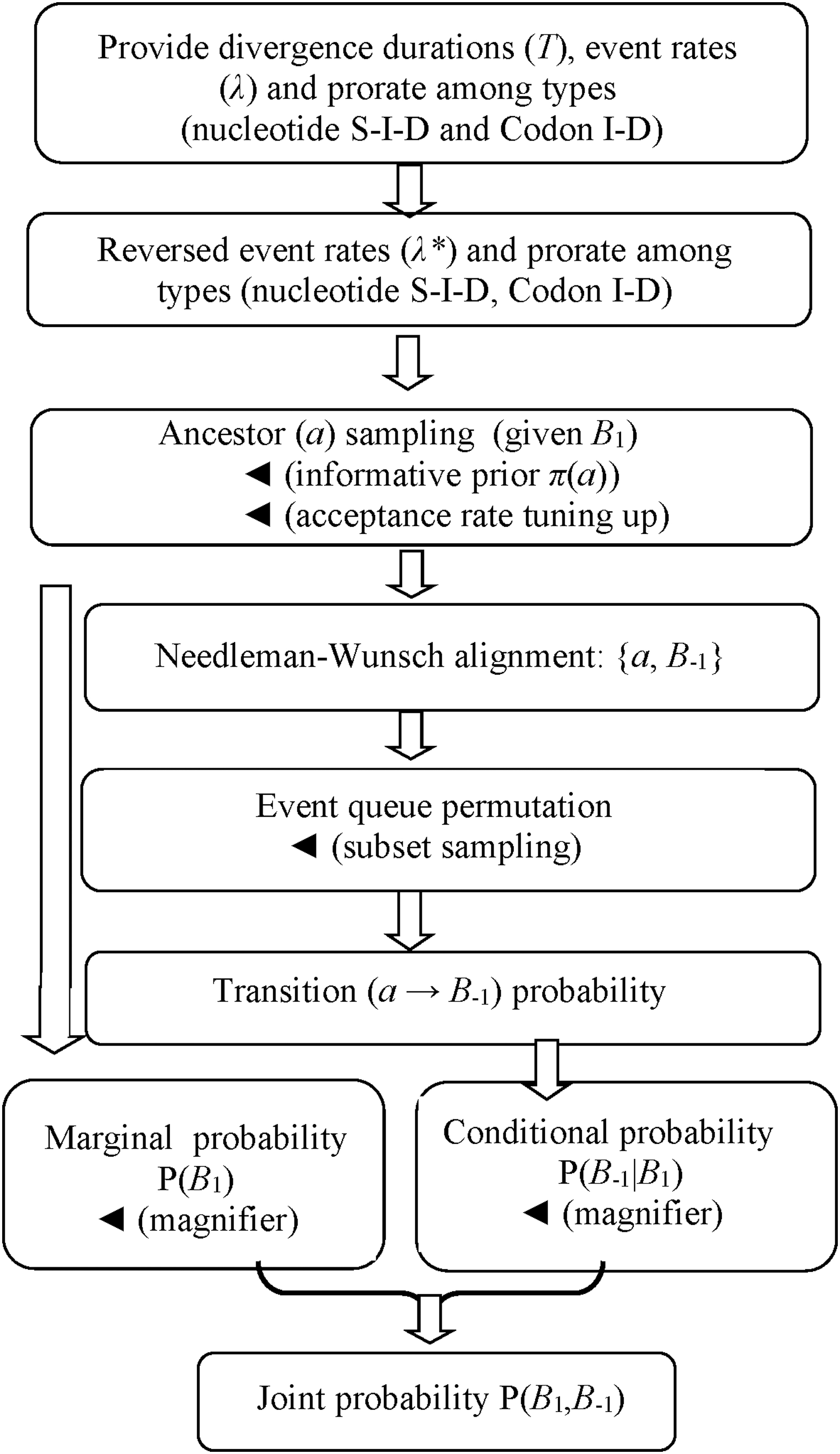
Computational procedure flowchart (the solid arrow represents an option).

2.4. Tree phylogeny

The preceding algorithms also apply to the tree phylogeny scenario (the right panel, Fig. 1; subject to minor adjustment). Specifically, the set probability is presented [similar to Eq. (7)] as $\begin{matrix} \begin{matrix} Pr (B_{1 : 3}) = Pr (B_{1 : 2} | B_{3}) Pr (B_{3}) \end{matrix} \\ = [\sum_{a} \sum_{r} Pr (B_{1 : 2} | r, a) Pr (r, a | B_{3})] \times Pr (B_{3}) \\ = [\sum_{a} \sum_{r} Pr (B_{1} | a) Pr (B_{2} | a) Pr (r, a | B_{3})] \times [\sum_{r} Pr (B_{3} | r) π (r)] . \end{matrix}$

Here, two latent sequences [the root (r) and the ancestor (a)] are to be sampled (given B₃). Once the prior distribution for the root (π(r)) is specified [similar to Eq. (8)], Pr(B₃) is obtained per Section 2.3.1 (with a replaced by r). The joint prior distribution (for the root and the ancestor) is presented as π(r,a) = π(r)Pr(a|r), where Pr(a|r) is dictated by the evolution models on the M process (Sections 2.1, 2.2.1, and 2.2.2). Given B₃, sampling a amounts to sampling r (given B₃, on the M* process, Section 2.3.2) followed by sampling a (given the sampled r, on the M process). The overall computational procedure is similar to the star evolution case.

2.5. Challenges from very short sequences

Compared with TKF91 model, our assumption and specification (Section 2.1) appear simpler. However, the price paid for not employing an equilibrium distribution for LCA (for attaining a reversible Markov process) may be suffering computational failure from handling very short sequences (e.g., <10 nucleotides) under certain configurations. For example, p_S = p_D = 0 amounts to site-letter-specific event rates of (0, p_I/4(l + 1),0)λ, which dictate that only nucleotide insertions occur on the M process (a→B) and transient null sequences (a) may subsequently occur on the M* process to prohibit exhibiting further deletions before reaching the terminal instant (t_B*). Moreover, pairwise alignment (Section 2.3.3) does not work on a null LCA sequence and an observed sequence (B₂ or B₃). Such a scenario challenges or may disable our proposed algorithms (Sections 2.2 and 2.3).

3. Results

3.1. A preliminary test on a set of short artificial sequences

The following three sequences {B_1:3} are artificially produced (assumed to evolve) from a specific ɑ = ATCGATCGATCGATCGATCG such that they have one, two, and three representative events, respectively.

B₁ = ATCGAT-GATCGATCGATCG (1 deletion),

B₂ = ATCGAT-GATTGATCGATCG (1 deletion, 1 substitution), and

B₃ = ATCGAT-GATTGATCTGATCG (1 deletion, 1 substitution, 1 insertion).

We let B₁ take the role of the reference sequence (B) [Eq. (13)]. In Eq. (8), we specify that Pr(l_a) = 1/21(10 ≤ l_a≤30) and π(i,k) = 1/4 for any k (1 ≤ i≤l_a) along with the Poisson process specification: λ = 0.1, t_B = 20, and (p_S,p_I,p_D) = (1,1,1)/3. We set H = 10^–12 and harvest N = 10³ ancestor samples (Section 2.3.2) with calculated probabilities presented in Table 2. We further check the probability profile (as λ varies) sensitivity to prorate weights by using another prorate weight vector (p_S,p_I,p_D) = (4,1,1)/6. The two correspondent sets of probabilities are compared in Figure 4, where the probability profile depends on the working prorate weights and the solid symbol along each profile represents the MLE for λ. The left panel has more outstanding (larger) probabilities (at MLE: λ = 0.07) along the profiles compared with the right panel. For one set of sequences, this small-scale study implies that a more realistic prorate (e.g., the left panel) likely leads to easier MLE for the rate (λ). We shall do large-scale (long sequences) studies in the following sections.

FIG. 4.

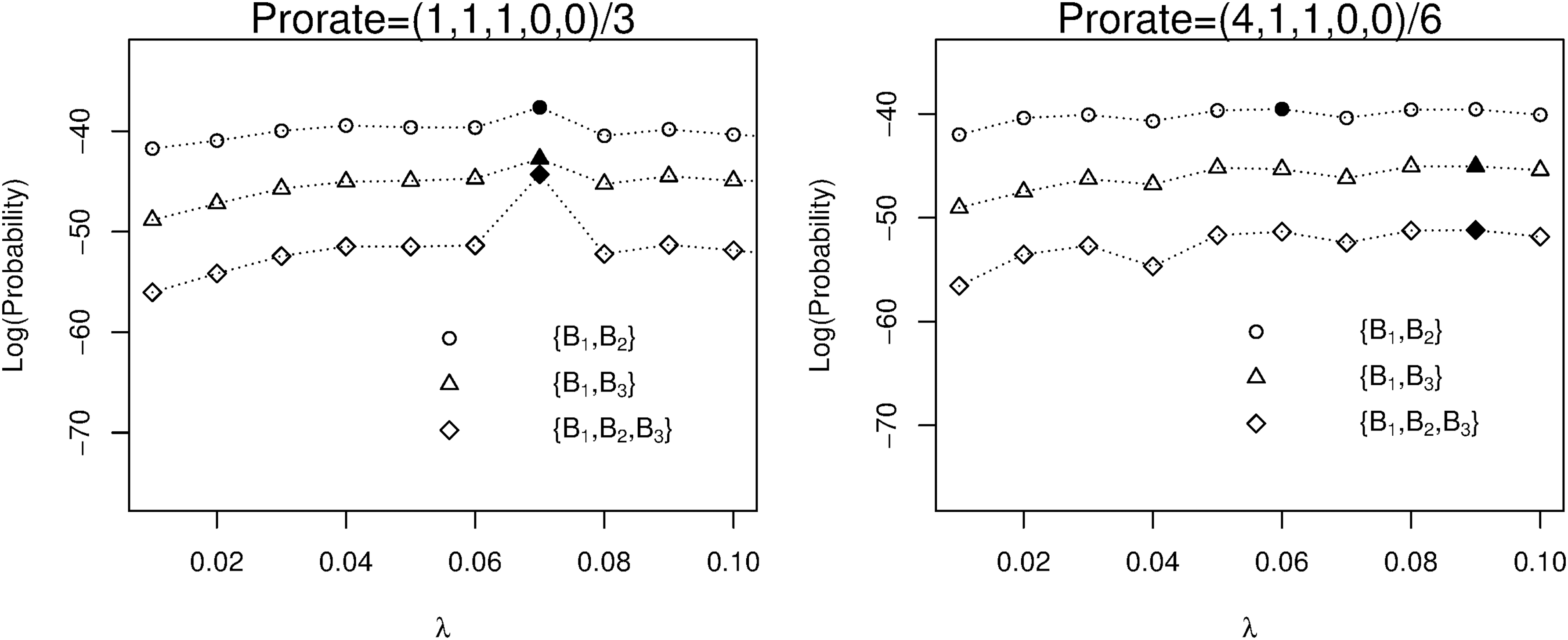
The probability profiles versus the generic event rate (λ). Obtained from short artificial sequences. The divergence time (t_B) = 2.0. The event rate prorates p = (1,1,1,0,0)/3 and p = (4,1,1,0,0)/6. The solid symbol along each profile represents the corresponding MLE for λ. MLE, maximum likelihood estimation.

Table 2.

Event Probabilities

	Event	Probability		Event	Probability
1	ɑ→B₀	1.35 E-01	3	B₂\|B₁	1.99 E-05
	ɑ→B₁	4.51 E-03		B₃\|B₁	2.05 E-07
	ɑ→B₂	5.14 E-05		B₂,B₃\|B₁	1.99 E-10
	ɑ→B₃	3.99 E-07
2	B ₀	4.75 E-14	4	{B₁, B₂}	2.99 E-18
	B ₁	1.50 E-13		{B₁, B₃}	3.08 E-20
	B ₂	1.67 E-13		{B₁, B₂, B₃}	2.99 E-23
	B ₃	4.25 E-14

The generic event rate (λ) = 0.1, the divergence time (t_B) = 20, and the prorate (p_S, p_I, p_D) = (1,1,1)/3. The ancestor length follows a uniform distribution in {10:30} where each nucleotide follows a tetranomial distribution across four letters {A,T,C,G} with equal chance. Part 1 shows the mutation (ancestor→observed sequence) probabilities, where the ancestor (a) = ATCGATCGATCGATCGATCG, B₀ = ATCG ATCGATCGATCGATCG (0 event), B₁ = ATCGATGATCGATCGATCG (1 event), B₂ = ATCGATGATTGATCG ATCG (2 events), and B₃ = ATCGATGATTGATCTGATCG (3 events). Part 2 shows the marginal probabilities of the observed sequences. Part 3 shows the conditional probabilities of the observed sequences given the reference sequence (B₁). Part 4 shows the joint probabilities of the sequence sets.

3.2. Real data: nuclear protein-coding sequences

3.2.1. Data description

Figure 5 lists eight hexapod species groups studied by Brandt et al. (2019), where each asexual lineage (without asterisk) stays with its closest sexual relative (with asterisk) in the unrooted cladogram along with sequence lengths and event counts for the orthologous nuclear protein-coding loci (GenBank number: MH602874-89, positive selection excluded). Neither mutational meltdown exists in the asexual lineages nor different purifying selections exist between two reproductive modes. BLAST multiple alignment takes MH602874 as the reference, and the most common mutation type is nucleotide substitution along with rare and randomly located nucleotide and/or codon insertion–deletions. For example, pair {1,1*} differs from 2* by at least one codon insertion (GAA) in the following portion extracted from multiple alignment of 16 orthologous sequences.

FIG. 5.

The unrooted cladogram with within-group event counts and rate (λ) estimates. The event counts are numbers of “nucleotide S-I-D, codon I-D, nucleotide identity” from aligning each pair (B_i, B_i*). The rate estimates are obtained by following Section 3.2.3.2.

(2*) MH602874 121 ATGCTTGGAAATGGGCGGCTTGAAGCGATGTGCTTTGATGG-AGTG——-AAACGGCTT 174

(1) MH602886 121 .….……C.….TT.G..G..C.….……C..-GACC——-…A.…A 174

(1*) MH602878 121 .….A.….…T..TT.A.….A.….T..C..C..-.…——-..GA..T.G 174

(Note: other species sequences or nucleotide sites are omitted)

(2*) MH602874 409—-AGTGATGA—-TGATGA—-A—-GATGA—-T—-GTTGATAATATCTGA 444

(1) MH602886 409—-.….…—-G.G…—-.—-.….—-.GAA..C.….C.….. 447

(1*) MH602878 409—-..C..C..—-A.GC..—-.—-.….—-.GAA..C.….…T… 447

The nuclear coding sequences have a simpler and more stochastic mutation mechanism than mtDNA (Adachi and Hasegawa,1992). The evolution mechanism underlying this data set roughly fits our model assumption and relevant probability calculation appears applicable.

3.2.2. Sequence (set) probabilities (marginal, conditional, joint)

Each group fits our model by sharing an LCA and tends to have a larger probability than a cross-group pair. Without the need of outgroup references, the noninformative π(a) induces the averaged probability that the pair would have diverged from certain LCA. We set: λ = 0.20, T = 100 (for each group), (l_min,l_max) = (440,450), m = 10³ (Section 2.2.2), the magnifier = 10³⁰⁰ (Section 2.3.1), the prorate (p_S,p_I,p_D,p_Ic,p_Dc) = (99,2/5,2/5,1/10,1/10)% (codon I-D is rarer than nucleotide I-D), the tuning parameter φ = 10⁻⁵ (Section 2.3.2) and harvest N = 10³ ancestor samples for Monte Carlo integration. In Table 3, the marginal sequence probability has a range of 10⁻²⁷²–10⁻²⁶⁹ without much difference across groups (Part 1). Conditional on B_i, P(B_i*|B_i) varies substantially across groups (10⁻¹⁸⁶–10⁻⁷⁹) and is 20–70 orders of magnitude larger than P(B_j|B_i) (cross-group pair {i, j}) (Part 2). “Negligible” probabilities arise from substantial codon insertions and/or deletions, for example, sequence 6(7) differs from 5(6) by three (four) codon insertion–deletions. The probabilities are compared (λ = 0.2 vs. 0.4) with larger ones (w/√) implying better λ specifications (Part 3). Pair set {{i,i*},i = 2,5,6} favors λ = 0.2 and set {{i,i*},i = 1,3,7,8} favors λ = 0.4 (roughly agrees with event count magnitudes in Fig. 5).

Table 3.

The Probabilities for a Real Data Set

	Event	Probability		Event	Probability
	Event	λ = 0.2	λ = 0.4	Event	λ = 0.2	λ = 0.4
1	{1}	(1.09, 3.11)	E-270	{5}	(1.17, 2.77)	E-270
	{1^*}	(1.14, 3.04)	E-270	{5^*}	(1.19, 2.75)	E-270
	{2}	(5.03, 8.64)	E-269	{6}	(4.89, 10.42)	E-269
	{2^*}	(4.71, 13.73)	E-269	{6^*}	(5.17, 11.49)	E-269
	{3}	(1.18, 3.86)	E-270	{7}	(4.33, 18.31)	E-272
	{3^*}	(1.15, 3.06)	E-270	{7^*}	(1.49, 3.01)	E-270
	{4}	(1.44, 3.06)	E-270	{8}	(4.34, 17.64)	E-272
	{4^*}	(1.17, 2.97)	E-270	{8^*}	(9.91, 37.63)	E-271
2	{1^* \| 1}	5.00E-172	2.82E-164√	{2 \| 1}	9.30E-191	3.81E-182
	{2^* \| 2}	1.66E-118√	8.07E-121	{3 \| 2}	1.75E-187	6.23E-177
	{3^* \| 3}	6.73E-141	2.69E-138√	{4 \| 3}	2.72E-199	Negligible
	{4^* \| 4}	3.15E-137	5.49E-138	{5 \| 4}	9.36E-177	2.28E-171
	{5^* \| 5}	8.28E-081√	2.08E-092	{6 \| 5}	Negligible
	{6^* \| 6}	6.88E-079√	9.24E-091	{7 \| 6}	Negligible
	{7^* \| 7}	1.44E-186	6.66E-176√	{8 \| 7}	Negligible
	{8 \| 8^*}	4.48E-169	2.01E-159√	{1\| 8^*}	Negligible
3	{1, 1^*}	5.45E-442	8.78E-434√	{1, 2}	1.01E-460	1.19E-451
	{2, 2^*}	8.33E-387√	6.97E-389	{2, 3}	8.33E-456	5.38E-445
	{3, 3^*}	7.96E-411	1.04E-407√	{3, 4}	3.21E-469	Negligible
	{4, 4^*}	4.54E-407	1.68E-407	{4, 5}	1.35E-446	6.96E-441
	{5, 5^*}	9.65E-351√	5.76E-362	{5, 6}	Negligible
	{6, 6^*}	3.37E-347√	9.63E-359	{6, 7}	Negligible
	{7, 7^*}	6.23E-458	1.22E-446√	{7, 8}	Negligible
	{8, 8^*}	4.43E-439	7.58E-429√	{8^*,1}	Negligible

The ancestor sequence length has a range of (l_min,l_max) = (440,450), the probability magnifier = 10³⁰⁰, and the number of ancestor samples (N) = 10³. The divergence time and generic event rate prorate are simply assumed to be T = 100 and p = (99,2/5,2/5,1/10,1/10)%. Sequence labels ({1:8},{1^*:8^*}) matches those in Figure 5. Part 1 shows marginal probabilities, Part 2 shows conditional probabilities, and Part 3 shows joint probabilities. Each event has two probabilities (the generic event rate λ = 0.2 or 0.4).

3.2.3. Estimate the generic event rates

3.2.3.1. Identical within-group rates

MLE estimate from a set of Poisson process instants often suffices for making statistical inference. The divergence time (T) is ∼40myo for Phasmatodea (pair{6,6*}) and ∼160 myo for Zygentoma (pair{7,7*}) (Brandt et al., 2019). For T = 40 and 160, we estimate an identical λ (for two sequences in each pair) by maximizing the joint probability under two prorates ((99,2/5,2/5,1/10,1/10) and (96,2,2,0,0)%) in Figure 6. Phasmatodea possesses arching profiles (as λ varies) and slightly favors the former prorate (with a higher maximal likelihood at λ = 0.43) over the latter one (with a slightly lower maximal likelihood at λ = 0.52). An opposite result appears for Zygentoma, which possesses unstable calculations at large λ (>0.4) (with the maximal likelihood at λ = 0.32). This comparison enhances the small-scale study (Section 3.1) and suggests to explore the joint space [the event rate (λ), the prorate (p)] for achieving the ultimate maximal likelihood.

FIG. 6.

The “log-probability vs. event rate (λ)” profile. The divergence times (T) for Phasmatodea and Zygentoma are 40 and 160, respectively. The ancestor sequence length range (l_min, l_max) = (440,450) and the number of ancestor samples (N) = 1000.

3.2.3.2. Distinct within-group rates

We now investigate the feasibility of estimating distinct rates for different species-specific sequences. We first use an artificial ancestor to simulate (T = 160) two sequences (B₁ (rate = 0.10), B₂ (rate = 0.50)). For each experimental rate λ₁, we use B₁ to sample LCA and find a value of λ₂, which maximizes Pr{B_1:2} (the left panel, Fig. 7). In the right panel, λ₁ is accurately estimated with λ₂ slightly underestimated, where a burn-in period (decreasing trend) may appear [taking B₁ = LCA (at λ₁ = 0) locates a λ₂ such that Tλ₂ ≈ the number of events between B₁ and B₂] with the real estimate appearing later on. We assign λ₁ and λ₂ (λ₁<λ₂) to pair{6*,6} (Phasmatodea, T = 40) and the maximal probability at (λ₁, λ₂) = (0.12, 0.78) (Fig. 8) substantially exceeds the identical-rate case (Fig. 6). Similar results apply to Zygentoma (T = 160) with maximal probability at (λ₁, λ₂) = (0.06, 0.55) (Fig. 9). However, the average of distinct rates ((λ₁ + λ₂)/2 = 0.45 or 0.31) is close to the identical rate (λ = 0.43 or 0.32). When we simply assume an identical λ ( = 0.20) for eight groups, the divergence times are estimated as T_1:8 = (19,14,16,14,10,10,20,18) × 10 (resolution = 10).

FIG. 7.

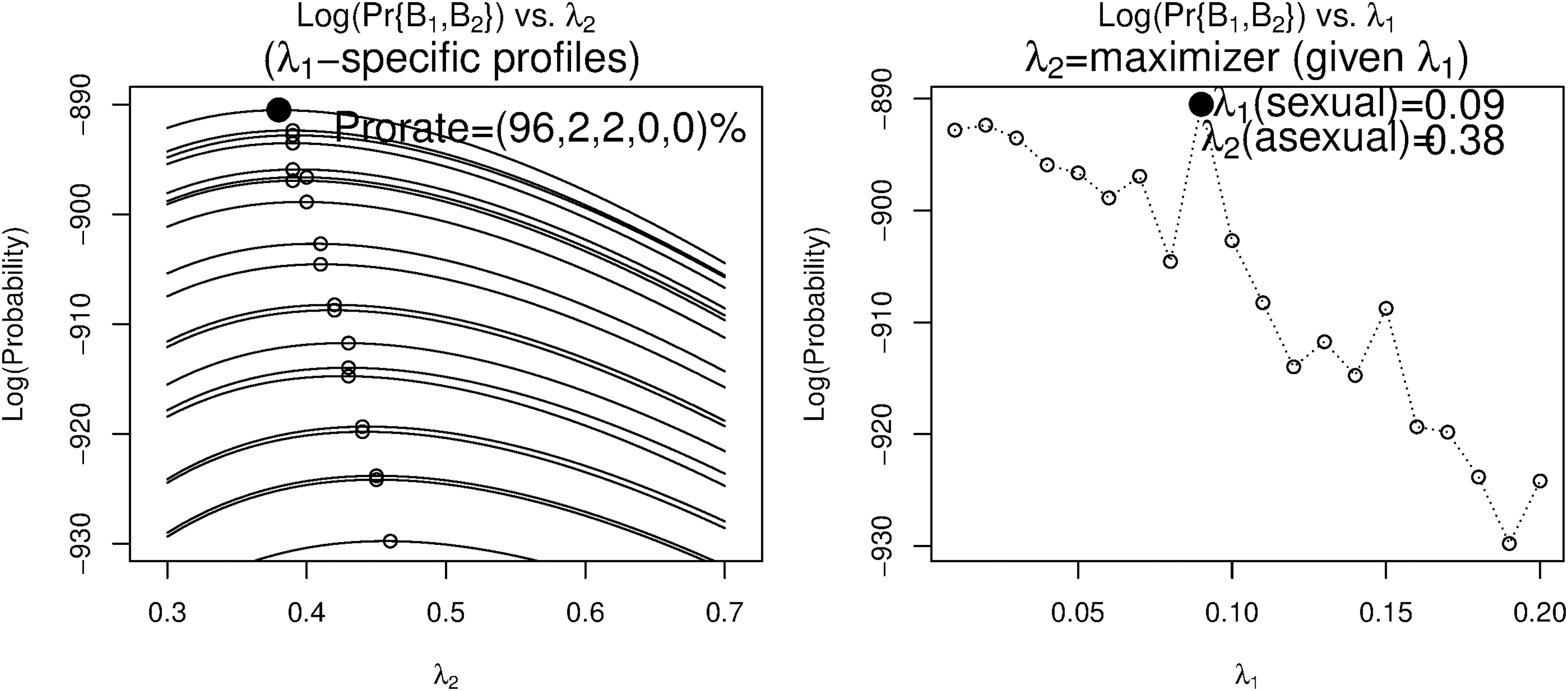
“Log-probability vs. event rate (λ2)” profiles (given event rate λ1) and “maximal log-probability (by λ2) vs. λ1” profiles. Obtained from simulated sequences. The divergence time (T) = 160, the ancestor sequence length range (l_min,l_max) = (440,450), and the number of ancestor samples (N) = 100.

FIG. 8.

“Log-probability vs. event rate (λ2)” profiles (given event rate λ1) and “maximal log-probability (by λ2) vs. λ1” profiles. Obtained from Phasmatodea sequences. The divergence time (T) = 40, the ancestor sequence length range (l_min,l_max) = (440,450), and the number of ancestor samples (N) = 100.

FIG. 9.

“Log-probability vs. event rate (λ2)” profiles (given event rate λ1) and “maximal log-probability (by λ2) vs. λ1” profiles. Obtained from Zygentoma sequences. The divergence time (T) = 160, the ancestor sequence length range (l_min,l_max) = (440,450), and the number of ancestor samples (N) = 100.

3.2.4. Biological insights

Nucleotide sequence mutation has complex biological mechanisms, which challenge statistical modeling and computation. Different species-specific nucleotide frequencies in the third codon position during amino acid substitution make the general reversible Markov model (with equilibrium assumption) inapplicable. The divergence at nonsynonymous sites (normalized for background substitution rates) (dN/dS) (Nei and Gojobori, 1986) is not robust (relying on likelihood and branch length estimates) and testing purifying selection effectiveness difference between reproductive modes of Zygentoma may be controversial (using dN/dS and CDC [codon deviation coefficient]) (Brandt et al., 2019). Our model omits certain complicated assumptions and/or components (e.g., letter-specific mutation probability, hydrophobicity fitness, time-varying rates). Moreover, since the match score ranking from BLAST multiple alignment may not completely agree with the cladogram, we simply use noninformative LCA priors rather than using an outgroup or internal reference. BLAST calculates statistical significance of alignment matches and we directly provide the joint probability P(B_1:2) to quantify between-species distance (e.g., two dissimilar sequences with negligible joint probability may not share an LCA). Once tree topology and divergence time (T_i)s are determined, any subtree with an overly small probability likely suffers from poor model fitting. Our results indicate that an identical within-group rate may not be realistic and distinct rates could be reasonably estimated using a small number of orthologous sequences.

4. Discussion

For long sequences (∼10³ nucleotides), we have considered a computational framework (e.g., LCA sampling, Monte Carlo integration, MLE of distinct rates among sequences) to improve evolution-based sequence analysis. Even if we do not require an outgroup reference to reconstruct the ancestor and/or gene gain–loss along sequences, a noninformative LCA prior still enables objective probability comparison and can potentially help to improve evolutionary tree construction. For very long sequences, segmentation may be an option for improving the computational efficiency. The sequence alignment algorithms (e.g., Needleman and Wunsch, 1970) on which our modeling and computational procedure depends mostly work for identifying substitutions and indels only. Of the alignment output, triple neighboring nucleotide insertions (deletions) are taken as one codon insertion (deletion) and a codon substitution arises from 1 to 3 independent nucleotide substitutions within the codon. Given these facts, the customized model (Section 2.2.2) involves codon I-D (on top of nucleotide S-I-D) and appears to work well for the nuclear protein-coding sequences (Section 3.2.1) in view of the event types identified from the multiple alignment therein. More complicated mechanisms (e.g., inversion, transposition) substantially challenge algorithm adjustment within our framework with causes including but not limited to the following: the involved segment length (along the whole sequence) per event varies and pairwise-alignment algorithms incorporating inversion-transposition identification are yet to come.

Footnotes

Acknowledgments

We appreciate the great efforts made by three anonymous referees who have contributed very constructive, insightful, and valuable comments, which have greatly improved our presentation. We are also grateful to Dr. Mona Singh (Editor-in-chief) for her very dedicated and patient coordination of the article reviewing process even after reformatting the article had taken us a prolonged time period during COVID-19 pandemic.

Author Disclosure Statement

The authors declare they have no conflicting financial interests.

Funding Information

The authors received no funding for this article.

References

Adachi

, and Hasegawa

1992. MOLPHY: Programs for molecular phylogenetics. In Computer Science Monographs, vol. 27. Institute of Statistical Mathematics, Tokyo, Japan.

Brandt

, Bast

, Scheu

, et al. 2019. No signal of deleterious mutation accumulation in conserved gene sequences of extant asexual hexapods. Sci. Rep. 9, 5338.

Camir

, Seidman

, Popic

, et al. 2020. Meltos: Multi-sample tumor phylogeny reconstruction for structural variants. Bioinformatics, 36, 1082–1090.

Jukes

T.H.

, and Cantor

C.R.

1969. Evolution of protein molecules, 21–132. In Munro, H.N., ed. Mammalian Protein Metabolism. Academic Press, New York.

Liu

, Chen

, Zhao

, et al. 2009. On calculating the probability of a set of orthologous DNA sequences. Adv. Appl. Bioinform Chem. 2, 37–48.

Needleman

S.B.

, and Wunsch

C.D.

1970. A general method applicable to the search for similarities in the amino acid sequence of two proteins. J. Mol. Biol. 48, 443–453.

Nei

, and Gojobori

1986. Simple methods for estimating the numbers of synonymous and nonsynonymous nucleotide substitutions. Mol. Biol. Evol. 3, 418–426.

Oliva

, Pulicani,S., Lefort

, et al. 2019. Accounting for ambiguity in ancestral sequence reconstruction. Bioinformatics, 35, 4290–4297.

Rigdon

S.E.

, and Basu

A.P.

2000. Statistical Methods for the Reliability of Repairable Systems. John Wiley & Sons, New York, NY.

10.

Suchard,M.A., Lemey,P., Baele,G., et al. 2018. A Bayesian phylogenetic and phylodynamic data integration using BEAST 1.10. Virus Evol. 4:vey016.

11.

Thorne

J.L.

, Kishino

, and Felsenstein

1991. An evolutionary model for maximum likelihood alignment of DNA sequences. J. of Mol. Evol. 33, 114–124.