A New ℓ 0 -Regularized Log-Linear Poisson Graphical Model with Applications to RNA Sequencing Data

Abstract

In this article, we develop a new ℓ ₀ -based sparse Poisson graphical model with applications to gene network inference from RNA-seq gene expression count data. Assuming a pair-wise Markov property, we propose to fit a separate broken adaptive ridge-regularized log-linear Poisson regression on each node to evaluate the conditional, instead of marginal, association between two genes in the presence of all other genes. The resulting sparse gene networks are generally more accurate than those generated by the ℓ ₁ -regularized Poisson graphical model as demonstrated by our empirical studies. A real data illustration is given on a kidney renal clear cell carcinoma micro-RNA-seq data from the Cancer Genome Atlas.

1. INTRODUCTION

High dimensional analysis in gene expression studies often requires identifying associations between genes. Scientists are usually interested in a sparse network, which provides biologists with insights into possible pathways from particular groups of genes (Dobra et al., 2004; Meinshausen and Bühlmann, 2006; Friedman et al., 2008). Multivariate Gaussian graphical models (Meinshausen and Bühlmann, 2006; Friedman et al., 2008) have been widely used to model continuous microarray data, since log ratios of the microarray gene expressions are approximately normally distributed after normalization. More recently, next generation high-throughput sequencing (RNA-seq) has become a popular data collection method for expression analysis (Dillies et al., 2013). Because RNA-seq gene expression data consist of counts of sequencing reads for each gene, researchers sought discrete probabilistic models, in favor of continuous Gaussian models, to describe the RNA-seq data (Srivastava and Chen, 2010; Witten, 2011; Allen and Liu, 2012; Gallopin et al., 2013; Choi et al., 2017; Imbert et al., 2018; Chiquet et al., 2019). Some of these previous studies address zero-inflated Poisson distributions (Choi et al., 2017), whereas others focus on multivariate Poisson models (Chiquet et al., 2019).

Owing to restrictions in assumptions imposed by some joint models, some seek to build network models using neighborhood selection (Meinshausen and Bühlmann, 2006; Allen and Liu, 2012). A key advantage of neighborhood selection, in contrast to a joint distribution model, is that each neighborhood sparse estimation can be done simply by a multivariate log-linear regression, and the regression model can be regularized conveniently by popular regularization methods such as ℓ₁-regularized Lasso. Neighborhood network selections assume a pair-wise Markov property (Lauritzen, 1996): conditional on all other variables, each variable follows a Poisson distribution, and is estimated locally through neighborhood selection (Meinshausen and Bühlmann, 2006) by fitting ℓ₁-regularized log-linear models (Allen and Liu, 2012). This Poisson graphical model based on neighborhood selection by Allen and Liu (2012) was recognized as one of the recent studies of graphical modeling specifically for discrete data with Poisson distributions, and it addresses conditional variable relationships without the need for a joint discrete distribution (Gallopin et al., 2013; Choi et al., 2017; Imbert et al., 2018; Chiquet et al., 2019). For the rest of the article, we address this model as L₁ log-linear graphical model (L₁-LLGM).

However, the L₁-LLGM method has some pitfalls because ℓ₁ regularization is known to lack oracle properties and tends to include unwanted noise variables (Zou, 2006; Zou and Zhang, 2009; Zhang, 2010). Consequently, the resulting estimated network is often not sparse enough when compared with the true underlying network structure. To mitigate this issue, Allen and Liu (2012) introduced a threshold to filter out small coefficients retained by ℓ₁-regularized log-linear regressions. We demonstrate in simulations that the inferred network is not robust with respect to the threshold level, and can sometimes have a very poor performance when a suboptimal threshold level is used. Unfortunately, no practical guidance is available in the literature on how to choose an appropriate threshold level for a given data set. In subsequent parts of the article, we employ the same assumptions (local Markov property) and settings (normalization, power transformation) of the L₁-LLGM, and propose a more refined estimation method for this model by adopting an ℓ₀-equivalent regularization.

We frame the goal of this article as an improvement over L₁-LLGM. To this aim, we developed and implemented an approximate ℓ₀-regularized log-linear graphical model (L₀-LLGM) for constructing sparse gene network from RNA-seq count data. We consider ℓ₀ regularization because it generally yields higher true-positive estimations than ℓ₁ regularization and has been shown to be more accurate for feature selection and parameter estimation (Lin et al., 2010, 2020; Shen et al., 2012, 2013). Because exact ℓ₀ regularization is computationally non-deterministic polynomial-time hardness (NP-hard) and only feasible for low dimension data, we adapt the recently developed broken adaptive ridge (BAR) method to approximate ℓ₀ regularization. Defined as the limit of an iteratively reweighted ℓ₂-regularization algorithm, the BAR method is an approximate ℓ₀-regularization method that enjoys the best of ℓ₀ and ℓ₂ regularizations with desirable selection, estimation, and grouping properties (Dai et al., 2018, 2020; Zhao et al., 2018, 2020; Kawaguchi et al., 2020b).

These desirable properties are important to our network analysis, as they offer a theoretical advantage of ℓ₀ regularization in our Poisson graphical model. Similar to L₁-LLGM, our proposed L₀-LLGM assumes a pair-wise Markov property and estimates gene network structures through a local sparse LLGM that evaluates conditional network correlations to each node. Specifically, at each step, a regularized Poisson log-linear model is fitted on one node, using BAR regularization to introduce sparsity. Nonzero coefficients estimate edges extending from the node. The stability approach to regularization selection (StARS) method (Liu et al., 2010) is used to select the regularization tuning parameters for the graphical model. Our empirical studies suggest that the proposed L₀-LLGM generally produces network structures closer to the true structure than those of L₁-LLGM, as measured by receiving operating characteristic (ROC) curves.

This article is organized as follows. In Section 4, we briefly review some gene expression normalization methods used before the network analyses, a step essential to all gene expression studies, introduce notations necessary for graphical model constructions, and review steps of LLGM model. In Section 2.2, we describe the proposed L₀-LLGM in detail. In Section 3, we illustrate the performance of L₀-LLGM in comparison with L₁-LLGM by simulating RNA-seq type of data from a few known network structures. We then describe a regularization parameter selection procedure for graphical models based on a stability algorithm in Section 2.3. Finally, we provide a real data illustration on kidney renal clear cell carcinoma (KIRC) micro-RNA (miRNA) data from the Cancer Genome Atlas (TCGA) (Collins and Barker, 2007) in Section 4.

2. METHODS

2.1. Data and notations

We define matrix X as the design matrix, where columns are variables and rows are samples. Matrix $X = (X_{1}, \dots, X_{p})$ is $n \times p$ , where $X_{j}$ ( $j = 1, \dots, p$ ) is the j-th column. Based on this design matrix, we aim to construct an undirected network model that would reveal conditional dependence between variables. It applies to count data that are assumed to have Poisson distributions. We then define the structure of the network as $G = {V, E}$ . $V$ is the set of all vertices in the network, where each vertex represents a variable (e.g., miRNA), quantified by a vector of the corresponding counts of aligned sequencing reads from each sample. $E$ represents the set of all edges connecting certain vertices.

2.2. ℓ₀-regularized log-linear Poisson graphical model through BAR

We consider a log-linear Poisson graphical model, which characterizes conditional Poisson relationships by assuming pair-wise Markov properties (Lauritzen, 1996). Specifically, we assume that for each $j = 1, \dots, p$ , the conditional distribution of column j, $X_{j} | X_{k} = x_{k} \forall k \neq j$ , is $p (X_{j} | X_{k} = x_{k} \forall k \neq j, B) \sim P o i s s o n (e^{\sum_{k \neq j} β_{j k} x_{k}}),$ (1)

where the intercept term $β_{j 0}$ is not included in the model, as we assume at this point RNA-seq data have been adjusted for sequencing depth in normalization steps, and $B = (β_{j k}, \forall k \neq j \in V)$ is a $p \times p$ adjacency matrix with each row vector of off-diagonal elements storing the corresponding log-linear Poisson regression coefficients.

The first step to neighborhood network selection method is to infer graphical networks by fitting the mentioned log-linear Poisson regression for every node j, $j = 1, \dots, p$ . Specifically, at each neighborhood selection step j ( $j = 1, \dots, p$ ), we determine only the potential edges connecting node j to all other nodes in the network. In addition, we couple the neighborhood selection method with the BAR, an approximate ℓ₀-regularization method, to induce sparsity as detailed in the following algorithm.

For each j, $j = 1, \dots, p$ , we begin with an initial ℓ₂-regularized (ridge) estimator of $β_{\neq j, j}$ ${\hat{β}}_{\neq j, j}^{(0)} = {argmin}_{β_{\neq j, j}} \{\frac{1}{n} \sum_{i = 1}^{n} [X_{i j} (X_{i, \neq j} β_{\neq j, j}) - e x p (X_{i, \neq j} β_{\neq j, j})] + ζ_{n} \sum_{k \neq j} β_{j k}^{2}\},$ (2)

where the first term is the $- 2$ log likelihood for the j-th log-linear Poisson regression model, $β_{\neq j, j}$ is a vector of $p - 1$ the corresponding regression coefficients, and $ζ_{n}$ is the ridge-regularization parameter. This initial step tuning parameter serves the purpose of giving iterative step a warm start. The BAR estimator defined hereunder has been shown to be robust for different choice of $ζ_{n}$ in various model settings [see, e.g., Kawaguchi et al. (2020b)—figure 1 and Li et al. (2021)—figure 7]. For a reasonable initial step estimation, we have set $ζ_{n}$ to $l o g (n)$ , where n is the sample size. We then subsequently update the estimator of $β_{\neq j, j}$ by fitting reweighted ℓ₂-regularized regressions with a tuning parameter $λ_{n}$ :

FIG. 1.

Simulation study for two network topologies: (A) scale free and (B) hub. For each network structure, we generated two data sets with two different number of observations, 200 and 500. A sequence of ℓ₀ or ℓ₁ penalization parameters was used to fit the modes on each data set. Predictions were evaluated by calculating true-positive and false-positive rates. These rates from both models were plotted for model comparisons (B, C, E, F). (B) and (C) Are two data sets, based on a scale-free network in (A), with simulated sample sizes equal to 200 and 500, respectively, while (E) and (F) are the same sample sizes based on a hub network in (D).

{\hat{β}}_{\neq j, j}^{(s)} = {argmin}_{β} {- 2 l (β) + λ_{n} \sum_{k \neq j} \frac{β_{j k}^{2}}{| {\hat{β}}_{j k}^{(s - 1)} |^{2}}}, s = 1, 2, \dots

(3)

The BAR (Kawaguchi et al., 2020a) estimator of $β_{\neq j, j}$ is defined as ${\hat{β}}_{\neq j, j} = {lim}_{s \to \infty} {\hat{β}}_{\neq j, j}^{(s)} .$

The BAR estimator has been shown to possess the oracle properties in the sense that with large probability, it estimates the zero coefficients as 0's and estimates the non-zero coefficients as well as the scenario when the true submodel is known in advance and a grouping property that highly correlated variables are naturally grouped together with similar coefficients (Kawaguchi et al., 2020a).

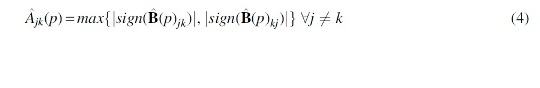
A nonzero element in coefficient estimate vector ${\hat{β}}_{\neq j, j}$ indicates that there is an estimated network connection (edge) between the corresponding node j and one of the nodes $1, \dots, p \neq j$ . The estimators ${\hat{β}}_{\neq j, j}$ , $j = 1, \dots, p$ , provide estimates of the off-diagonal elements of adjacency matrix $B$ . Diagonal elements of $B$ can be set to either missing or unity, since it is not meaningful to evaluate a node's relationship with itself. Note that $B$ is also not necessarily symmetric, as fitting regressions on element i and j does not guarantee the same zero or nonzero coefficient corresponding to the same node. To deal with this nonsymmetric issue, we chose to estimate based on the union of network edge constructions,

Theoretically, whether to use the union or intersection of each network edge based on its two neighborhood selections concerning its two nodes is asymptotically identical (Meinshausen and Bühlmann, 2006). This less conservative approach of estimating by unions remains consistent with previous neighborhood selection Poisson graphical model literature (Allen and Liu, 2012). In other words, if either one of the two local log-linear regressions concerning the two nodes i and j produces a nonzero estimate, it implies conditional dependency. Consequently the network estimate specifies an edge between nodes i and j. Therefore, estimated adjacency matrix is always symmetrical. Estimated coefficients, $\hat{B}$ , is then transformed to an adjacency matrix, $Â$ , by simply changing all nonzero estimates to 1, namely, $Â = s i g n | \hat{B} |$ .

Lastly, we note that for each j, $j = 1, \dots, p$ , the BAR estimator ${\hat{β}}_{\neq j, j}$ is defined as the limit of a sequence of reweighted ridge estimators. In a numerical implementation, one will stop the BAR iterations for ${\hat{β}}_{\neq j, j}$ when a prespecified convergence criterion is met. In our implementation, the algorithm stops at step s when $m a x_{k \neq j} | {\hat{β}}_{j k}^{(s)} - {\hat{β}}_{j k}^{(s - 1)} | < a$ , and we set ${\hat{β}}_{\neq j, j} = {{\hat{β}}_{j k}^{(s)} I (| {\hat{β}}_{j k}^{(s)} | > a), k \neq j}$ , where a is the convergence criterion threshold, which can be set to a reasonably small value, such as $10 e - 18$ . Our empirical studies indicate that one may use a slightly larger value to reduce the number of iterations with essentially no difference in the resulting estimator. We set $a = 10 e - 6$ as the default value in our R implementation. We emphasize that threshold a is not a regularization parameter. It is comparable with the stopping rule for a Lasso gradient descent implementation. It is purely for implementing the computer algorithm, as it serves as a stop mechanism for numerical convergence. This is not to be confused with the artificial threshold in L₁-LLGM (Allen and Liu, 2012; Wan et al., 2016), which, in the R package, was imposed after Lasso gradient descent stopping rule, effectively “weeding out” small, but converged, Lasso coefficients.

2.3. Selecting regularization parameters through StARS criterion

The sparsity and performance of the network largely depend on the regularization parameter $λ_{n}$ in Equation (3), which directly determines the number of estimated edges that stay in the network. Note that most of the popular data-driven tuning parameter selection methods such as Akaike's information criteria (AIC), Bayesian information criteria (BIC), and cross-validation require finding the log likelihood of the joint distribution, which all local neighborhood log-linear Poisson models do not have. Thus, we opt to select regularization parameters utilizing StARS (Liu et al., 2010). The StARS selection criterion selects the regularization parameter based on given model stability. It does so by subsampling rows, without replacement, into blocks of equal sizes.

Specifically, let K be the number of subsamples that we draw, and let X^k be a subsample from the design matrix X, where $k \in {1, \dots, K}$ . Liu et al. (2010) suggest that, in order for assumptions of StARS algorithm to be met, a reasonable choice of the subsample size is $b = ⌊ 10 \sqrt{n} ⌋$ . In our case of neighborhood Poisson graphical model, individual full models are fitted on each subsample. For any edge between two given vertices, we will have obtained K estimates on the same edge, each from a subsample already mentioned. First, we define an inverse of the tuning parameter $Λ = 1 ∕ λ_{n}$ . For any edge connecting vertices s and t, let the estimate from subsample S_j, using regularization parameter $Λ$ , be $ψ_{s t}^{Λ} (S_{j})$ . $ψ_{s t}^{Λ} (S_{j}) = 1$ if there is an edge between s and t, and $ψ_{s t}^{Λ} (S_{j}) = 0$ if the model does not estimate that there is an edge at $(s, t)$ . The stability of model predictions on this specific position is then given by ${\hat{θ}}_{s t} (Λ) = \frac{1}{N} \sum_{j = 1}^{N} ψ_{s t}^{Λ} (S_{j}) .$ (5)

A potential issue here with estimator ${\hat{θ}}_{s t} (Λ)$ is that the measure is not monotonic, rendering future model assessment and comparisons difficult. The model is stable when estimates from different subsamples all tend to give a value of 1 or 0. In other words, ${\hat{θ}}_{s t} (Λ)$ is the most stable when it is close to 0 or 1, and the least stable when it is close to $0.5$ . Therefore, we use a monotonized stability measure, ${\hat{ξ}}_{s t} (Λ) = 2 {\hat{θ}}_{s t} (Λ) (1 - {\hat{θ}}_{s t} (Λ)) .$ (6)

Lastly, an overall stability measure is then calculated by evaluating the mean of all edge-specific instabilities, ${\hat{D}}_{s t} (Λ) = \frac{\sum_{s < t} {\hat{ξ}}_{s t} (Λ)}{(\begin{matrix} p \\ 2 \end{matrix})} .$ (7)

When $Λ$ is close to 0, meaning regularization parameter $λ$ is large, L₀-LLGM produces an empty graph. As all subsample estimates are sparse, the instability shall approach 0. As $Λ$ increases, the subsample networks become denser and more volatile. Instability consequently increases till it peaks. ${\hat{D}}_{s t} (Λ)$ will start decreasing as the regularization parameter becomes smaller and the networks become dense. As the networks become almost fully connected, the instability measure will again approach 0, since all subsamples give similar estimates. Therefore, instabilities are expected to have a bell shape when plotted against penalization parameter. Authors who proposed StARS criterion also suggested a way to select the optimal sparsity given the least instability. Users first need specify an instability threshold, $γ$ . Then the algorithm should select the largest penalization parameter, that is, the sparsest network, with instability score below or equal to $γ$ .

The performance instability criterion is supported theoretically by the Theorem of Partial Sparsistency (Liu et al., 2010), which states that under suitable regularity conditions, the estimated set of edges is expected to contain the set of edges in the true underlying model as n approaches infinity.

We developed an R package for implementing L₀-LLGM, which can be found at repository https://github.com/caeseriousli/prBARgraph.git.

3. SIMULATIONS

In this section, we demonstrate the performance of the BAR Poisson graphical model (L₀-LLGM) versus ℓ₁ Poisson graphical model (L₁-LLGM) through simulations. To evaluate model fit, we measure prediction accuracy by the true-positive rates and false-positive rates. The true-positive rate is defined as the portion of correctly predicted edge out of total number of edges predicted. For instance, if a predicted network has a total of 80 edges, out of which 40 exist in the underlying true network, then the true-positive rate is $40 ∕ 80 = 0.5$ in this case. False-positive rate, however, is calculated by dividing the number of incorrectly predicted edges by the total number of nonexisting edges in the true network.

3.1. Simulating correlated Poisson networks

To generate simulation data for model comparison, we adapt the same method introduced in Allen and Liu (2012). Again, let n be the number of observations and p the number of elements (genes). We first generate independent Poisson samples: Y, a $n \times (p + p (p - 1) ∕ 2)$ matrix, where $Y_{i j} \sim^{i . i . d} P o i s s o n (λ_{t r u e})$ . Then we randomly generate a noise term E, an $n \times p$ matrix where $E_{i j} \sim^{i . i . d} P o i s s o n (λ_{n o i s e})$ .

Furthermore, using the underlying true network, we construct a structure matrix,

where A is the adjacency matrix corresponding to the network, $t r i (A)$ is a vectorized, $(p \times (p - 1) ∕ 2) \times 1$ , upper triangular part of adjacency matrix A , and $1_{(p)}$ here is a column vector of which each element is equal to 1. The purpose of the identity vector is to expand $t r i (A)$ into a $p \times (p (p - 1) ∕ 2)$ matrix, which is used to calculate element-wise product with a permutation matrix, _P, with dimensions $(p (p - 1) ∕ 2) \times p$ . The permutation matrix is constructed by permuting indices of all possible pairs of vertices across its rows. For example, if the first row of the permutation matrix, P , represents an edge connecting node number 1 and node number 2, then the first two elements of the first row, which contains a total of p elements, will be 1. The rest of elements in the first row are 0. Concordantly, P has $p (p - 1) ∕ 2$ rows because a network can potentially have a total of distinct $p (p - 1) ∕ 2$ edges. Note that the order of permutations in P have to match the order we expand the adjacency matrix, namely, $t r i (A)$ . In addition, $:$ denotes the block matrix structure with the p × p identity matrix on the left. Finally, we simulate the design matrix by $X = Y B + E$ .

3.2. Model comparison

When compared with nondiscrete models, such as graphical Lasso (Friedman et al., 2008), the L₁-LLGM model has already been numerically demonstrated to have as good or better prediction accuracy for simulated Poisson data (Allen and Liu, 2012). In this article, as the major innovation is an L₀ BAR regularization, we will focus on comparing L₀-LLGM with L₁-LLGM. We will move on to adopt simulation setup similar to Allen and Liu (2012). Specifically, we simulated RNA sequencing data based on two common network topologies, hub and scale free. The data are randomly generated using methods introduced in Section 3.1. For each topology, we have constructed a network consisting of 50 nodes. For each topology we generate two data sets, with 200 and 500 independent samples, respectively. We further note that, sample sizes no greater than 500 in simulations are common for most RNA-seq studies (Gallopin et al., 2013; Choi et al., 2017; Imbert et al., 2018; Chiquet et al., 2019).

For each model, both the L₀-LLGM and L₁-LLGM methods are performed on the simulated data, using StARS criterion to determine the regularization parameters. For L₁-LLGM, we considered a set of four different values for the additional sparsity threshold (“th”), specified by L₁-LLGM implementations as a necessary step (Wan et al., 2016), to investigate its effects on the resulting estimated network. With both true-positive and false-positive measurements defined in the beginning of Section 3, we construct ROC curves to compare the performance of L₀-LLGM in comparison with L₁-LLGM. Figure 1 shows the ROC curves generated under two different topologies, scale free (Fig. 1A) and hub (Fig. 1D), each consisting of 50 nodes. We observe that L₀-LLGM consistently outperformed L₁-LLGM, especially in high specificity regions. The advantage of L₀-LLGM is more evident for hub topology. Furthermore, it is clear that the performance of L₁-LLGM can vary greatly depending on the choice of its sparsity threshold. The optimal choice of this threshold depends on the underlying topology and sample sizes. For any given false-positive rate, L₀-LLGM yields a model with more correctly estimated connections. L₁-LLGM, in contrast, could potentially lose nodes that are important to the structure of the network shown in Figure 1.

Lastly, we validate the mentioned findings in replications. Owing to limitations of ROC plot visualizing multiple network fits, we summarize 40 replications in box plots. In Figures 2 and 3, L₀-LLGM and L₁-LLGM are fitted to 40 randomly generated data sets from scale-free and hub topologies, respectively. At each replication, both the topology and data set are randomly generated, and each data set has sample size $n = 500$ .

FIG. 2.

Simulation study for scale-free topology with sample size $n = 500$ . Topologies and data sets are randomly generated 100 times for each model. For all repetitions, area under the curve for true-positive rates and false-positive edge estimation percentages are summarized in box plots. Area under the curve is defined as the area under true-positive versus false-positive rate curve as regularization parameter increases, same as that of Figure 1. These repeated simulations are based on randomly generated scale-free topologies with 200 sample sizes and 50 number of nodes, corresponding to the same specifications in Figure 1B. Both the topology and data set are simulated randomly at each repetition.

FIG. 3.

Simulation study for hub topology with sample size $n = 500$ . Topologies and data sets are randomly generated 100 times for each model. For all repetitions, area under the curve for true-positive rates and false-positive edge estimation percentages are summarized in box plots. Area under the curve is defined as the area under true-positive versus false-positive rate curve as regularization parameter increases, same as that of Figure 1. These repeated simulations are based on randomly generated hub topologies with 200 sample sizes and 50 number of nodes, corresponding to the same specifications as in Figure 1E. Both the topology and data set are simulated randomly at each repetition.

4. APPLICATION OF L₀-LLGM TO KIRC miRNA-SEQ DATA

High throughput sequencing (second generation RNA sequencing) returns millions of short reads of RNA fragments, which have varying lengths ranging from ∼25 to possibly 300 bp paired-end reads (Chhangawala et al., 2015). These reads are usually mapped to the genome and the data are in the form of non-negative counts of the RNA fragment reads (Witten, 2011). LLGM models can be applied to any data that are assumed to have Poisson distributions. For RNA-seq data specifically, a normalization pipeline is required before data analysis. For comparison purposes, we follow the same normalization pipeline as Wan et al. (2016); Allen and Liu (2012), which consists of the following major steps: (1) adjusting for sequencing depth, (2) biological entities (e.g., genes, miRNAs) with low counts or low variances are filtered out, (3) vectors with potential over-dispersion are transformed using a power transformation to transform the data closer to Poisson distribution (Li et al., 2012; Wan et al., 2016). The normalization steps can be performed by R package XMRF (Wan et al., 2016). We defer the detailed procedures and justifications of this specific pipeline for RNA-seq Poisson graphical models to Wan et al. (2016).

We then fitted the proposed method on the KIRC miRNA data set from The Cancer Genome Atlas. The data set was downloaded from TCGA data portal (https://portal.gdc.cancer.gov) (Collins and Barker, 2007). It contains 1881 miRNAs and 616 samples. Before the normalization pipeline, we filtered out miRNAs that have all zero read counts throughout all samples, resulting in 1502 miRNAs left (20.15% of miRNAs with low counts). Then we normalize the rest of the data using XMRF package developed for L₁-LLGM (Wan et al., 2016). For demonstration purposes of this article, we specify the R package to keep top 100 miRNAs with the most variance (i.e., look at top miRNAs that vary the most). Minimum read count is set to be no less than 20, the suggested default (Allen and Liu, 2012; Wan et al., 2016). This keeps ∼6.7% of miRNAs. We then move on to focus on conditional relationships between these 100 miRNAs with the largest variance and reasonable read counts. We then fit L₀-LLGM using our R package, along with L₁-LLGM, implemented by XMRF (Wan et al., 2016), with an StARS instability threshold of $γ = 0.01$ (choosing the largest regularization while maintaining at least “99% stability”). Figures 4 and 5 show the resulting L₀-LLGM and L₁-LLGM network estimates, respectively. Figure 5 contains four panels, each with a different L₁-LLGM artificial threshold. Network estimates could be drastically different depending on the threshold. Table 1 provides miRNA annotations for use of node numbers in Figures 4 and 5.

FIG. 4.

L₀-LLGM KIRC miRNA data: estimated network generated by fitting an L₀-LLGM model on KIRC miRNA data from TCGA database. The penalization parameter was chosen by setting an StARS estimation instability threshold of 0.01. KIRC, kidney renal clear cell carcinoma; L₀-LLGM, ℓ₀-regularized log-linear graphical model; miRNA, micro-RNA; StARS, stability approach to regularization selection; TCGA, the Cancer Genome Atlas.

FIG. 5.

L₁-LLGM KIRC miRNA data: estimated network generated by fitting an L₁-LLGM model on KIRC miRNA data from TCGA database. The penalization parameter was chosen by setting an StARS instability threshold of 0.01. In addition, a further artificial threshold (“th”) to fine tune the L₁-LLGM model. This figure shows four network estimates by varying the th threshold.

Table 1.

Micro-RNA Network Annotation

ID	miRNA	ID	miRNA	ID	miRNA	ID	miRNA
1	hsa-let-7a-1	26	hsa-mir-1178	51	hsa-mir-124-1	76	hsa-mir-126
2	hsa-let-7a-2	27	hsa-mir-1179	52	hsa-mir-124-2	77	hsa-mir-1260a
3	hsa-let-7a-3	28	hsa-mir-1180	53	hsa-mir-124-3	78	hsa-mir-1260b
4	hsa-let-7b	29	hsa-mir-1181	54	hsa-mir-1243	79	hsa-mir-1262
5	hsa-let-7c	30	hsa-mir-1182	55	hsa-mir-1244-1	80	hsa-mir-1263
6	hsa-let-7d	31	hsa-mir-1185-1	56	hsa-mir-1244-2	81	hsa-mir-1264
7	hsa-let-7e	32	hsa-mir-1185-2	57	hsa-mir-1245a	82	hsa-mir-1265
8	hsa-let-7f-1	33	hsa-mir-1193	58	hsa-mir-1245b	83	hsa-mir-1266
9	hsa-let-7f-2	34	hsa-mir-1197	59	hsa-mir-1246	84	hsa-mir-1267
10	hsa-let-7g	35	hsa-mir-1199	60	hsa-mir-1247	85	hsa-mir-1268b
11	hsa-let-7i	36	hsa-mir-1200	61	hsa-mir-1248	86	hsa-mir-1269a
12	hsa-mir-1-1	37	hsa-mir-1203	62	hsa-mir-1249	87	hsa-mir-1269b
13	hsa-mir-1-2	38	hsa-mir-1204	63	hsa-mir-1250	88	hsa-mir-127
14	hsa-mir-100	39	hsa-mir-122	64	hsa-mir-1251	89	hsa-mir-1270
15	hsa-mir-101-1	40	hsa-mir-1224	65	hsa-mir-1252	90	hsa-mir-1271
16	hsa-mir-101-2	41	hsa-mir-1225	66	hsa-mir-1253	91	hsa-mir-1272
17	hsa-mir-103a-1	42	hsa-mir-1226	67	hsa-mir-1254-1	92	hsa-mir-1273c
18	hsa-mir-103a-2	43	hsa-mir-1227	68	hsa-mir-1254-2	93	hsa-mir-1273h
19	hsa-mir-105-1	44	hsa-mir-1228	69	hsa-mir-1255a	94	hsa-mir-1275
20	hsa-mir-105-2	45	hsa-mir-1229	70	hsa-mir-1256	95	hsa-mir-1276
21	hsa-mir-106a	46	hsa-mir-1231	71	hsa-mir-1257	96	hsa-mir-1277
22	hsa-mir-106b	47	hsa-mir-1234	72	hsa-mir-1258	97	hsa-mir-1278
23	hsa-mir-107	48	hsa-mir-1236	73	hsa-mir-125a	98	hsa-mir-128-1
24	hsa-mir-10a	49	hsa-mir-1237	74	hsa-mir-125b-1	99	hsa-mir-128-2
25	hsa-mir-10b	50	hsa-mir-1238	75	hsa-mir-125b-2	100	hsa-mir-1281

miRNA, micro-RNA.

It is observed from Figures 4 and 5 that the two model results reveal some similar structures, including the hub surrounding center, mir-10b (node 25). However, L₀-LLGM produces a less visually “chaotic” network, in comparison with L₁-LLGM. For instance, L₀-LLGM outlines a clean scale-free topology with minimal cyclic loops. L₁-LLGM, however, frequently exhibits loops even in sparse network estimates, possibly due to unwanted noises from ℓ₁ regularization. From Figure 5, as we increase the “artificial threshold” for L₁-LLGM used in XMRF package, to some extent it helps reducing these noise edges.

However, during this process, we observe that this user-imposed threshold also filtered out lower degree nodes (weaker signal), such as the hub miRNAs surrounding node 25. For example, in Figure 5A1, with no artificial threshold, L₁-LLGM identifies hub center node 25 (mir-10b), which agrees with L₀-LLGM in Figure 4. As the threshold increases, plots in Figure 5A2–B2 show a decreasing degree in hub center node 25. In Figure 5B2, almost entire hub is filtered out by this threshold along with noise. This observation parallels to the simulation section (Fig. 1), where the true-positive rates can be reduced by the artificial threshold, losing important network structures. These preliminary observations suggest that L₀-LLGM is potentially more capable of separating signal from noise, which is consistent with our simulation results depicted in Figure 1.

Although a graphical model alone is not enough to make any further conclusions on gene interactions inference, we focus, in particular, on highly connected miRNAs (i.e., hub nodes). Some of the hub miRNAs revealed by the L₀-LLGM network were previously known to be associated with each other, and with certain cancers. For example, the center of the largest hub, gene mir-10b in Figure 4 is known to be associated with cancers such as bladder cancer and proteoglycans cancer. Based on literature studies, this RNA was known to be highly expressed in metastatic hepatocellular carcinomas, in contrast to those without metastasis (Ma et al., 2010). Our network results are based on the data from patients with adenomas and adenocarcinomas from project KIRC. It is connected to numerous miRNAs, including several cluster centers known to be associated with cancer suppressing. RNA named hsa-let-7b, for example, identified as a subcluster connected to the hub center mir-10b, a previously known putative cancer suppressor, is found to play a key role in chemoresistance in renal cells from carcinoma cases (Peng et al., 2015). Together with another cluster center RNA, named miR-126 and hsa-let-7b are both identified as crucial biomarkers for identifying renal cell carcinoma (Jusufović et al., 2012; Yin et al., 2014; Carlsson et al., 2019). Our graphical model successfully identifies important miRNAs that align with published biological findings regarding such miRNAs.

We also performed additional analyses using different StARS instability thresholds $γ = 0.005$ and $γ = 0.05$ . The findings are consistent with what have been discussed previously for $γ = 0.01$ and thus not included here.

5. DISCUSSION

We have proposed and implemented an approximate L₀-LLGM for constructing sparse gene network from RNA-seq count data. This approach uses a neighborhood Poisson graphical model, which offers a more comprehensive set of predictions, has less constraints on the Poisson distributions of each element, and is less sensitive to changes of individual genes, than a joint distribution model. Sparsity is achieved through the BAR penalization, a surrogate ℓ₀ regularization with established oracle properties for selection and estimation. Our simulations in Section 3 show that, in general, L₀-LLGM offers theoretically more accurate estimates than L₁-LLGM. It reaches a high level of true-positive rate faster, without accumulating a high rate of false estimates. L₀-LLGM also spares users the need of selecting an additional sparsity threshold after the regularization tuning parameter has already been selected by StARS. This brings more consistency and reproducibility to the graphical model.

Our simulations considered two types of network topologies, namely scale-free and hub topologies, and found that both L₀-LLGM and L₁-LLGM tend to perform better under scale-free topologies as compared with hub. However, because graphical models could potentially give drastically different results under various topologies, it would be of interest to consider more topologies in future studies.

It is worth noting that although this article has focused on the $p < n$ case, the proposed methodology can be easily extended to high dimensional settings where $p > n$ by coupling the BAR penalization with a sure screening procedure (Fan and Lv, 2008; Zhao and Li, 2012; Xu and Chen, 2014; Barut et al., 2016). Combining the BAR penalization with a sure screening procedure for high dimensional settings and its statistical guarantees have been studied for a variety of models including linear model (Dai et al., 2018), generalized linear models (Li et al., 2021), and survival models (Zhao et al., 2018, 2020; Kawaguchi et al., 2020b). Future studies are warranted to further investigate the empirical performance of the two-step procedure for network inference in high dimensional settings.

We acknowledge that, for model applications in RNA-seq data, the network in itself often is not enough to draw definitive inference on complex gene interactions. Often a network serves as a first step in identifying clusters, under the assumptions that genes interact with each other in hubs (Friedman, 2004). One can modularize clustered genes through methods such as dynamic tree cutting. These modules can subsequently be used for gene enrichment analyses (Langfelder and Horvath, 2008).

Footnotes

AUTHOR DISCLOSURE STATEMENT

The authors declare they have no competing financial interests.

FUNDING INFORMATION

The research of G.L. was partly supported by National Institute of Health Grants P30CA-16042, UL1TR000124-02, and P50CA211015.

References

Allen

G.I.

, and Liu

2012. A log-linear graphical model for inferring genetic networks from high-throughput sequencing data, pp. 1–6. In 2012 IEEE International Conference on Bioinformatics and Biomedicine. IEEE, New York, NY, USA.

Barut

, Fan

, and Verhasselt

2016. Conditional sure independence screening. J. Am. Stat. Assoc. 111, 1266–1277.

Carlsson

, Christiansen

, Davidsson

, et al. 2019. The potential role of mir-126, mir-21 and mir-10b as prognostic biomarkers in renal cell carcinoma. Oncol. Lett. 17, 4566–4574.

Chhangawala

, Rudy

, Mason

C.E.

, et al. 2015. The impact of read length on quantification of differentially expressed genes and splice junction detection. Genome Biol. 16, 1–10.

Chiquet

, Robin

, and Mariadassou

2019. Variational inference for sparse network reconstruction from count data, pp. 1162–1171. In Chaudhuri, K., and Salakhutdinov, R., eds. Proceedings of the 36th International Conference on Machine Learning, Volume 97 of Proceedings of Machine Learning Research. PMLR.

Choi

, Gim

, Won

, et al. 2017. Network analysis for count data with excess zeros. BMC Genet. 18, 1–10.

Collins

F.S.

, and Barker

A.D.

2007. Mapping the cancer genome. Sci. Am. 296, 50–57.

Dai

, Chen

, and Li

2020. The broken adaptive ridge procedure and its applications. Statistica Sin. 30, 1069–1094.

Dai

, Chen

, Sun

, et al. 2018. Broken adaptive ridge regression and its asymptotic properties. J. Multivar. Anal. 168, 334–351.

10.

Dillies

M.-A.

, Rau

, Aubert

, et al. 2013. A comprehensive evaluation of normalization methods for illumina high-throughput RNA sequencing data analysis. Brief. Bioinform. 14, 671–683.

11.

Dobra

, Hans

, Jones

, et al. 2004. Sparse graphical models for exploring gene expression data. J. Multivar. Anal. 90, 196–212.

12.

Fan

, and Lv

2008. Sure independence screening for ultrahigh dimensional feature space. J. R. Stat. Soc. B Stat. Methodol. 70, 849–911.

13.

Friedman

, Hastie

, and Tibshirani

2008. Sparse inverse covariance estimation with the graphical lasso. Biostatistics, 9, 432–441.

14.

Friedman

2004. Inferring cellular networks using probabilistic graphical models. Science, 303, 799–805.

15.

Gallopin

, Rau

, and Jaffrézic

2013. A hierarchical Poisson log-normal model for network inference from RNA sequencing data. PLoS One, 8, e77503.

16.

Imbert

, Valsesia

, Le Gall

, et al. 2018. Multiple hot-deck imputation for network inference from RNA sequencing data. Bioinformatics, 34, 1726–1732.

17.

Jusufović

, Rijavec

, Keser

, et al. 2012. let-7b and mir-126 are down-regulated in tumor tissue and correlate with microvessel density and survival outcomes in non–small–cell lung cancer. PLoS One, 7, e45577.

18.

Kawaguchi

E.S.

, Shen

J.I.

, Suchard

M.A.

, et al. 2020a. Scalable algorithms for large competing risks data. J. Comput. Graph. Stat. pp. 1–23.

19.

Kawaguchi

E.S.

, Suchard

M.A.

, Liu

, et al. 2020b. A surrogate ℓ ₀ sparse cox's regression with applications to sparse high-dimensional massive sample size time-to-event data. Stat. Med. 39, 675–686.

20.

Langfelder

, and Horvath

2008. WGCNA: An R package for weighted correlation network analysis. BMC Bioinform. 9, 1–13.

21.

Lauritzen

S.L.

1996. Graphical Models, volume 17. Clarendon Press, Oxford, England.

22.

, Witten

D.M.

, Johnstone

I.M.

, et al. 2012. Normalization, testing, and false discovery rate estimation for RNA-sequencing data. Biostatistics, 13, 523–538.

23.

, Peng

, Kawaguchi

, et al. 2021. A scalable surrogate l0 sparse regression method for generalized linear models with applications to large scale data. J. Stat. Plan. Inference, 213, 262–281.

24.

Lin

, Li

, and Lian

2020. A novel recommendation system via l0-regularized convex optimization. Neural Comput. Appl. 32, 1649–1663.

25.

Liu

, Roeder

, and Wasserman

2010. Stability approach to regularization selection (StARS) for high dimensional graphical models, pp. 1432–1440. In Advances in Neural Information Processing Systems. Vancouver, British, Columbia, Canada.

26.

, Reinhardt

, Pan

, et al. 2010. Therapeutic silencing of mir-10b inhibits metastasis in a mouse mammary tumor model. Nat. Biotechnol. 28, 341.

27.

Meinshausen

, and Bühlmann

2006. High-dimensional graphs and variable selection with the lasso. Ann. Stat. 34, 1436–1462.

28.

Peng

, Mo

, Ma

, et al. 2015. let-7b and let-7c are determinants of intrinsic chemoresistance in renal cell carcinoma. J. Surg. Oncol. 13, 175.

29.

Shen

, Pan

, and Zhu

2012. Likelihood-based selection and sharp parameter estimation. J. Am. Stat. Assoc. 107, 223–232.

30.

Shen

, Pan

, Zhu

, et al. 2013. On constrained and regularized high-dimensional regression. Ann. Inst. Stat. 65, 807–832.

31.

Srivastava

, and Chen

2010. A two-parameter generalized Poisson model to improve the analysis of RNA-seq data. Nucleic Acids Res. 38, e170–e170.

32.

Wan

Y.-W.

, Allen

G.I.

, Baker

, et al. 2016. XMRF: An R package to fit Markov networks to high-throughput genetics data. BMC Syst. Biol. 10, 69.

33.

Witten

D.M.

2011. Classification and clustering of sequencing data using a Poisson model. Ann. Appl. Stat. 5, 2493–2518.

34.

, and Chen

2014. The sparse MLE for ultrahigh-dimensional feature screening. J. Am. Stat. Assoc. 109, 1257–1269.

35.

Yin

, Bai

, Song

, et al. 2014. Differential expression of serum mir-126, mir-141 and mir-21 as novel biomarkers for early detection of liver metastasis in colorectal cancer. Chin. J. Cancer, 26, 95.

36.

Zhang

C.-H.

2010. Nearly unbiased variable selection under minimax concave penalty. Ann. Stat. 38, 894–942.

37.

Zhao

, Sun

, Li

, et al. 2018. Variable selection for recurrent event data with broken adaptive ridge regression. Can. J. Stat. 46, 416–428.

38.

Zhao

, Wu

, Li

, et al. 2020. Simultaneous estimation and variable selection for interval-censored data with broken adaptive ridge regression. J. Am. Stat. Assoc. 115, 204–216.

39.

Zhao

S.D.

, and Li

2012. Principled sure independence screening for Cox models with ultra-high-dimensional covariates. J. Multivar. Anal. 105, 397–411.

40.

Zou

2006. The adaptive lasso and its oracle properties. J. Am. Stat. Assoc. 101, 1418–1429.

41.

Zou

, and Zhang

H.H.

2009. On the adaptive elastic-net with a diverging number of parameters. Ann. Stat. 37, 1733.

A New ℓ 0 -Regularized Log-Linear Poisson Graphical Model with Applications to RNA Sequencing Data

Abstract

1. INTRODUCTION

2. METHODS

2.1. Data and notations

2.2. ℓ0-regularized log-linear Poisson graphical model through BAR

2.3. Selecting regularization parameters through StARS criterion

3. SIMULATIONS

3.1. Simulating correlated Poisson networks

3.2. Model comparison

4. APPLICATION OF L0-LLGM TO KIRC miRNA-SEQ DATA

5. DISCUSSION

Footnotes

AUTHOR DISCLOSURE STATEMENT

FUNDING INFORMATION

References

2.2. ℓ₀-regularized log-linear Poisson graphical model through BAR

4. APPLICATION OF L₀-LLGM TO KIRC miRNA-SEQ DATA