Cotranscriptional Kinetic Folding of RNA Secondary Structures Including Pseudoknots

Abstract

Computational prediction of ribonucleic acid (RNA) structures is an important problem in computational structural biology. Studies of RNA structure formation often assume that the process starts from a fully synthesized sequence. Experimental evidence, however, has shown that RNA folds concurrently with its elongation. We investigate RNA secondary structure formation, including pseudoknots, that takes into account the cotranscriptional effects. We propose a single-nucleotide resolution kinetic model of the folding process of RNA molecules, where the polymerase-driven elongation of an RNA strand by a new nucleotide is included as a primitive operation, together with a stochastic simulation method that implements this folding concurrently with the transcriptional synthesis. Numerical case studies show that our cotranscriptional RNA folding model can predict the formation of conformations that are favored in actual biological systems. Our new computational tool can thus provide quantitative predictions and offer useful insights into the kinetics of RNA folding.

1. INTRODUCTION

Ribonucleic acid (RNA) is a biopolymer composed of nucleotides with bases adenine (A), cytosine (C), guanine (G), and uracil (U). The synthesis of an RNA molecule from its DNA template is initiated when the corresponding RNA polymerase binds to the DNA promoter region. RNA has been shown to serve diverse functions in a wide range of cellular processes, such as regulating gene expression and acting as an enzymatic catalyst (Storz, 2002; Collins and Penny, 2009), and has also recently been used as an emerging material for nanotechnology (Jasinski et al., 2017).

Computational prediction of RNA secondary structures given their sequences is often based on the estimation of changes in free energy, which postulates that thermodynamically an RNA strand will fold into a conformation that yields the minimum free energy (MFE) [see, e.g., Fallmann et al. (2017) for a review on the topic]. The energy of an RNA secondary structure can be modeled as the sum of energies of strand loops flanked by base pairs. The loop energy parameters have been measured experimentally and are detailed in a nearest neighbor parameter database (NNDB) (Turner and Mathews, 2009). Methods grounded in the thermodynamic framework, for example, the Zuker algorithm by Zuker and Stiegler (1981) and its extensions (Zuker, 1989; Mathews et al., 1999), can be used to compute pseudoknot-free MFE secondary structures effectively in a bottom-up manner. Recent attempts to extend the Zuker algorithm to find MFE secondary structures with certain classes of pseudoknots are also proposed (Rivas and Eddy, 1999; Akutsu, 2000; Dirks and Pierce, 2003; Reeder and Giegerich, 2004; Chen et al., 2009); however, finding MFE structures with pseudoknots given a general energy model is an NP-complete problem (Lyngsø and Pedersen, 2000).

The kinetic approach (Flamm et al., 2000) is an alternative way to study the RNA folding process. It models the folding as a random process where the additions/deletions of base pairs in the current structure are assigned probabilities proportional to the respective changes in free energy values. A folding pathway of a sequence is then generated by executing stochastic simulation (Mironov and Lebedev, 1993; Flamm et al., 2000; Dykeman, 2015). We refer to Marchetti et al. (2017) for a comprehensive review on stochastic simulation and recent work (Thanh et al., 2014, 2016; Marchetti et al., 2016; Thanh et al., 2017) for state-of-the-art stochastic simulation techniques. Each simulation runs on a given RNA sequence can produce a list of possible structures that it can fold into. Such dynamic view of RNA folding allows one to capture cases where local conformations are progressively folded to create metastable structures that kinetically trap the folding, thus complementing the prediction of equilibrium MFE structures produced by the thermodynamic approach.

The study of RNA structure formation often assumes that the folding process starts from a fully synthesized open strand, the denatured state. However, experimental evidence (Pan and Sosnick, 2006; Watters et al., 2016) has shown that RNA starts folding already concurrently with the transcription. The nucleotide transcription speed varies from 200 nt/s (nucleotides per second) in phages, to 20–80 nt/s in bacteria, and to 5–20 nt/s in humans (Pan and Sosnick, 2006). The RNA dynamics also occur over a wide range of time scales where base pairing takes about 10⁻³ ms; structure formation is about 10–100 ms; and kinetically trapped conformations can persist for minutes or hours (Al-Hashimi and Walter, 2008). One consequence of considering cotranscriptional folding is that the base pairs at the 5′ end of the RNA strand will form first, whereas the ones at the 3′ end can only be formed once the transcription is complete, which leads to structural asymmetries. Cotranscriptional folding can thus form transient structures that are only present for a specific time period and involved in distinct roles. For instance, gene expression when considering such transient conformations of RNA during cotranscriptional folding can exhibit oscillation behavior (Bratsun et al., 2005). We refer to the review by Lai et al. (2013) for further discussion on the importance of cotranscriptional effects.

In this work, we extend the kinetic approach to take into account cotranscriptional effects and pseudoknots on the folding of RNA secondary structures at single-nucleotide resolution. Our contribution is twofold. First, we explicitly consider the elongation of RNA during transcription as a primitive action in the model. The time when a new nucleotide is added to the current RNA chain is specified by the transcription speed of the RNA polymerase enzyme. The RNA strand in our modeling approach can elongate with newly synthesized nucleotides added to the sequence and fold simultaneously. To handle the transcription events, we propose an exact stochastic simulation method, the CoStochFold algorithm, to correct the folding pathway. Our method is thus able capture the effects of cotranscriptional folding at single-nucleotide resolution instead of approximating it as in previous approaches (Mironov and Kister, 1986; Flamm et al., 2000; Zhao et al., 2011; Proctor and Meyer, 2013; Hua et al., 2018). Second, our algorithm allows the formation of pseudoknots, which are important for understanding RNA functions. To cope with the challenge in evaluating the energy of pseudoknotted RNA structures, we adapt the NNDB model (Dirks and Pierce, 2003; Andronescu et al., 2010) to calculate their energy values. It is worth noting that determining a reasonable energy model for RNA structures with pseudoknots is still an open question (Lyngsø and Pedersen, 2000; Chen et al., 2009). However, the advantage of our strategy in comparison with other approaches, for example, adapting polymer theory in protein folding (Dill, 1999) to evaluate energy of pseudoknots (Isambert and Siggia, 2000), is that in the future when experimental data for pseudoknot parameters are established we can readily apply the simulation without revalidating parameters of the energy model. In addition, we facilitate the computation of energy of RNA structures with pseudoknots by employing a motif tree representation. This concept extends the coarse-grained tree representation of pseudoknot-free RNA structures, for example, Hofacker and Stadler (2005), to allow also pseudoknotted motifs.

The rest of the article is organized as follows. Section 2 reviews some background on kinetic folding of RNA. In Section 3, we present our work to extend the model of RNA folding to incorporate the transcription process and handle the formation of pseudoknots. Section 4 reports our numerical experiments on case studies. Concluding remarks are in Section 5.

2. BACKGROUND ON KINETIC FOLDING

Let S_n be a linear sequence of length n of four bases A, C, G, and U in which the 5′ end is at position 1 and the 3′ end is at position n. A base at position i may form a pair with a base at j, denoted by (i, j), if they form a Watson–Crick pair A-U, G-C, or a wobble pair G-U. A secondary structure formed by intramolecular interactions between bases in S_n is a list of base pairs $(i, j)$ with $i < j$ satisfying constraints: (1) the ith base and jth base must be separated by at least 3 (unpaired) bases, i.e., $j - i > 3$ ; (2) for any base pair $(k, l)$ with $k < l$ , if $i = k$ , then $j = l$ ; and (3) for any base pair $(k, l)$ with $k < l$ , if $i < k$ , then $i < k < l < j$ . The first condition prevents the RNA backbone from bending too sharply. The second one prevents the forming of tertiary structure motifs, such as base triplets and G-quartets. The last constraint ensures that no two base pairs intersect, that is, there are no pseudoknots. We will relax this constraint in Section 3 to allow for the formation of pseudoknots during the folding.

Let $Ω_{S_{n}}$ be the set of all possible secondary structures formed by S_n. Consider a secondary structure $x \in Ω_{S_{n}}$ . It can be represented compactly as a string of dots and brackets (Fig. 1). Specifically, for a base pair $(i, j)$ , an opening parenthesis “(” is put at ith position and a closing parenthesis “)” at jth position. Finally, unpaired positions are represented by dots “.”. The dot-bracket representation is unambiguous because the base pairs in a secondary structure do not cross each other. An alternative method of representing RNA secondary structures is arc diagram. The arc diagram depicts an RNA structure as a horizontal line from 5′ end (left) to 3′ end (right) with arcs connecting nucleotides at positions in the sequence to show respective base pairs in the structure. The advantage of the arc diagram is that it can represent RNA structures, for example, pseudoknotted structures, which are difficult or impossible to visualize as planar diagrams. Figure 1a–c, respectively, shows the dot bracket, the arc diagram, and the graphical visualization of tRNA molecule.

FIG. 1.

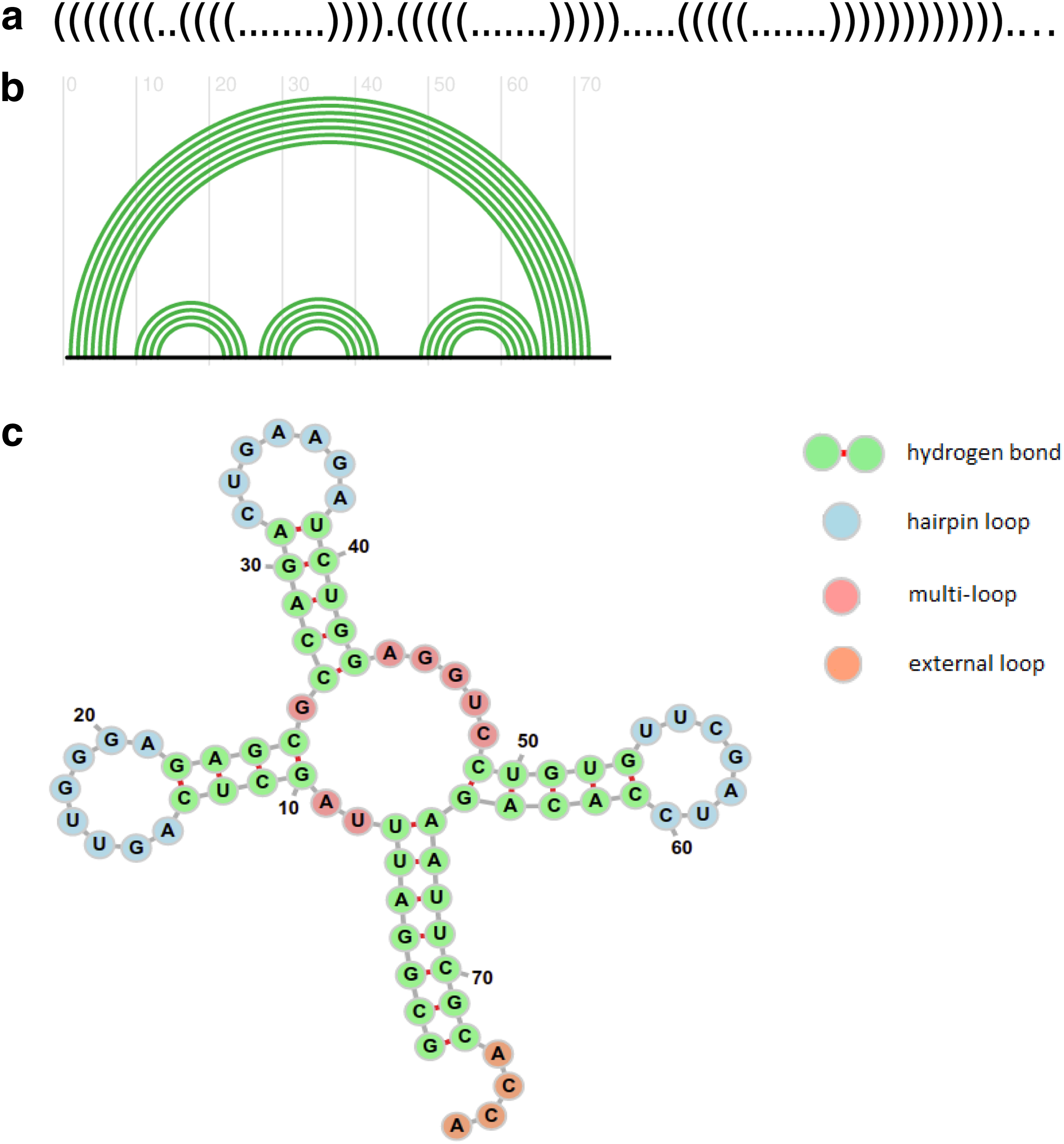
Representation of the tRNA molecule in (a) dot-bracket notation, (b) arc diagram, and (c) graphical visualization. The graphical visualization is made by the Forna tool (Kerpedjiev et al., 2015). RNA, ribonucleic acid.

The free energy of x can be estimated by the nearest neighbor model (Mathews et al., 1999), in which the free energy of an RNA secondary structure is taken to be the sum of energies of components flanked by base pairs. Formally, for a base pair $(i, j)$ in x, we say that base k, $i < k < j$ , is accessible from $(i, j)$ if there is no other base pair $(i', j')$ such that $i < i' < k < j' < j$ . The set of accessible bases flanked by base pair $(i, j)$ is called the loop $L (i, j)$ . The number of unpaired bases in a loop $L (i, j)$ is its size, whereas the number of enclosed base pairs determines its degree. Based on these properties, loops $L (i, j)$ can be classified as stacks (or stems), hairpins, bulges, internal loops, and multi-loops (or multi-branch loops). The unpaired bases that are not contained in loops constitute the exterior (or external) loop $L_{e}$ .

A secondary structure x is thus uniquely decomposed into a collection of loops $x = \cup_{(i, j)} L (i, j) \cup L_{e}$ . Based on this decomposition, the free energy G_x (in kcal) of secondary structure x is computed as: $G_{x} = \sum_{(i, j)} G_{L (i, j)} + G_{L_{e}},$ (1)

where $G_{L (i, j)}$ is the free energy of loop $L (i, j)$ . Experimental energy values for $G_{L (i, j)}$ are available in the nearest neighbor database (Turner and Mathews, 2009).

Let $y \in Ω_{S_{n}}$ be a secondary structure derived directly from x by an intramolecular reaction between bases i and j in x. Commonly, three operations on a pair of bases, referred to as the move set (Fig. 2), are defined (Flamm et al., 2000):

FIG. 2.

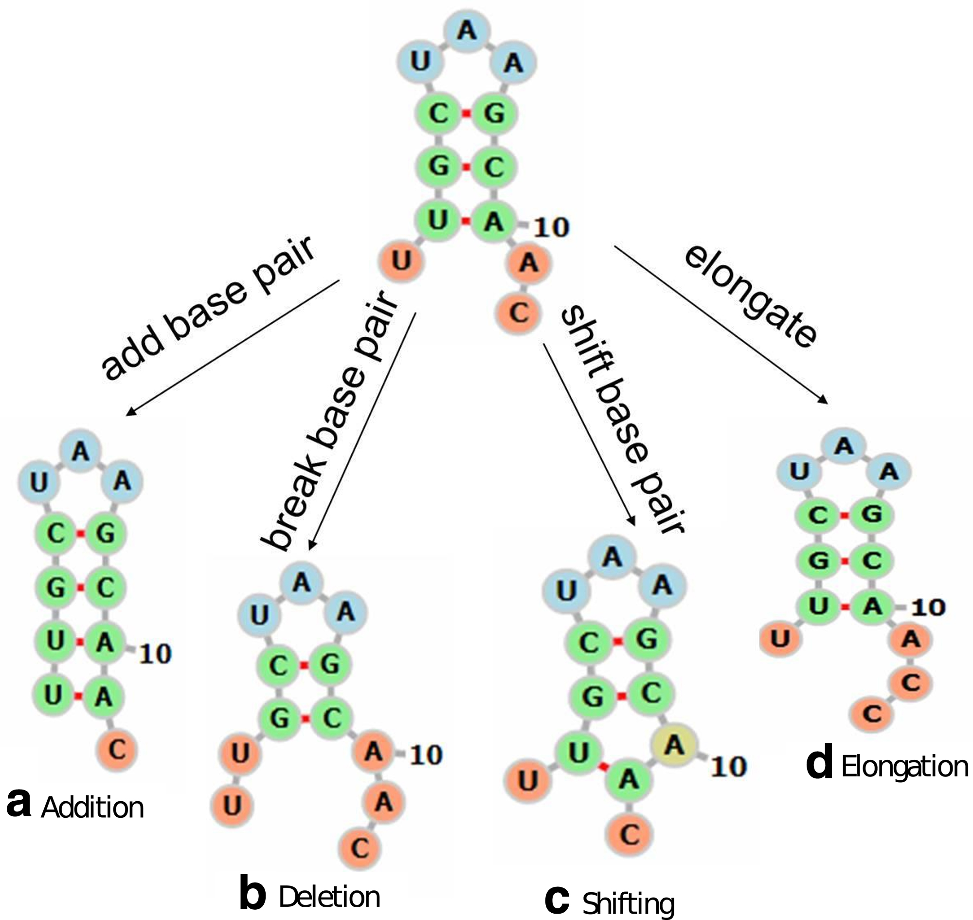
Extended move set consisting of (a) addition, (b) deletion, (c) shifting, and (d) elongation. The elongation move models the transcription process extending the current RNA chain with a new nucleotide at the 3′ end.

Addition: y is derived by adding a base pair that joins bases i and j in x that are currently unpaired and eligible to pair.

Deletion: y is derived by breaking a current base pair $(i, j)$ in x.

Shifting: y is derived by shifting a base pair $(i, j)$ in x to form a new base pair $(i, k)$ or $(k, j)$ .

Let $k_{x \to y}$ be the rate (probability per time unit) of the transition from x to y. In a conformation x, the RNA molecule may wander vibrationally around its energy basin for a long time, before it surmounts an energy barrier to escape to a conformation y in another basin. The dynamics of the transition from x to y characterizes a rare event in Molecular Dynamics. Here, we adopt the coarse-grained kinetic Monte Carlo approximation (Metropolis et al., 1953; Kawasaki, 1966) and model the transition rate $k_{x \to y}$ as: $k_{x \to y} = k_{0} e^{- Δ G_{x y} ∕ 2 R T},$ (2)

where T is absolute temperature in Kelvin (K), $R = 1.98717 \times 1 0^{- 3} (k c a l \times K^{- 1} \times m o l^{- 1})$ is the gas constant, and $Δ G_{x y} = G_{y} - G_{x}$ denotes the difference between free energies of x and y. The constant k₀, normally taking values in the range 10³ to 10⁴, provides a calibration of time.

Let $P (x, t)$ be the probability that the system is at conformation x at time t. The dynamics of $P (x, t)$ is formulated by the (chemical) master equation (Marchetti et al., 2017) as: $\frac{d P (x, t)}{d t} = \sum_{y \in Ω_{S_{n}}} [k_{y \to x} P (x, t) - k_{x \to y} P (x, t)] .$ (3)

Analytically solving Equation (3) requires to enumerate all possible states x and their neighbors y. The size of the state space $∥ Ω_{S_{n}} ∥ \sim n^{- 3 ∕ 2} α^{n}$ with $α = 1.8488$ increases exponentially with the sequence length n, and the number of neighbors of x is in order of $O (n^{2})$ (Hofacker et al., 1998). Thus, due to the high dimension of the state space, solving Equation (3) often involves numerical simulation.

Let $P (y, τ | x, t)$ be the probability that, given current structure x at time t, x will fold into y in the next infinitesimal time interval $[t + τ, t + τ + d τ)$ . We have $P (y, τ | x, t) = k_{x \to y} e^{- k_{x} τ} d τ,$ (4)

where $k_{x} = \sum_{y \in Ω_{S_{n}}} k_{x \to y}$ is the sum of transition rates to single-move neighbors of x. Equation (4) lays down the mathematical framework for stochastic RNA folding. Integrating Equation (4) with respect to $τ$ from 0 to $\infty$ , the probability that x moves to y is $k_{x \to y} ∕ k_{x}$ . Summing Equation (4) over all possible states $y \in Ω_{S_{n}}$ , it shows the waiting time $τ$ until the transition occurs and follows an exponential distribution $E x p (k_{x})$ . These facts are the basis for our kinetic folding algorithm called StochFold presented as Algorithm 1. We note that StochFold shares the structure of the earlier algorithm Kinfold (Flamm et al., 2000) and its improvements (Thanh and Zunino, 2014; Dykeman 2015).

Algorithm 1: StochFold

Require: initial RNA conformation s₀ and ending time

T_{m a x}

1: initialize

x = s_{0}

and time

t = 0

2: repeat

3: enumerate next possible conformations of the current conformation x and put into set Q

4: compute the transition rate

k_{x \to y}

for each

y \in Q

and total rate

k_{x} = \sum_{y \in Q} k_{x \to y}

5: select next conformation

y \in Q

with probability

k_{x \to y} ∕ k_{x}

6: sample waiting time to the next folding event

τ \sim E x p (k_{x})

7: set

x = y

and

t = t + τ

8: until

t \geq T_{m a x}

3. COTRANSCRIPTIONAL KINETIC FOLDING OF RNA

The folding of an RNA strand adapts immediately to new nucleotides synthesized during the transcription. The kinetic approach described in Section 2 cannot capture the effects of such cotranscriptional folding because it considers only interactions between bases already present in the sequence. We outline in this section an approach to incorporating these effects in the simulation. The transcription process is explicitly taken into account by extending the move set with the new operation of elongation. Our extended move set thus comprises four operations: addition, deletion, shifting, and elongation. The first three operations are defined as in the previous section. In elongation, the current RNA chain increases in length and a newly synthesized nucleotide is added to its 3′ end. Figure 2 illustrates the extended move set.

Under the extended move set, we define two event types: folding event and transcription event. A folding event is an internal event that occurs when one of the three operations, addition, deletion, or shifting, is applied to a base pair of the current sequence. A transcription event happens when the elongation operation is applied. It is an external event whose rate is specified by the transcription speed of the RNA polymerase enzyme. The occurrences of transcription events break the Markovian property of transitions between conformations. This is because when a new nucleotide is added to the current RNA conformation, the number of next possible conformations increases. The waiting time of the next folding event also changes, and thus, a new folding event has to be recomputed.

Algorithm 2 outlines how the CoStochFold algorithm handles this situation. The key element of CoStochFold (lines 8–15) is a race where the event having the smallest waiting time will be selected to update the current RNA conformation. More specifically, suppose the current structure is x at time t. Let $τ_{e}$ be the waiting time to the next folding event and $τ_{t r a n s}$ the waiting time to the next transcription event. Assuming that no events occur earlier, $τ_{e}$ has an exponential distribution with rate k_x, which is the sum of all transition rates of applying addition, deletion, and shifting operations to base pairs in x. For simplifying the computation of $τ_{t r a n s}$ , we assume that it is the expected time to transcribe one nucleotide. Let $N_{t r a n s}$ be the (average) transcription speed of the polymerase. We compute $τ_{t r a n s}$ as: $τ_{t r a n s} = 1 ∕ N_{t r a n s} .$ (5)

Thus, given current time t, the next folding event will occur at time $t_{e} = t + τ_{e}$ and, respectively, the transcription event where a new nucleotide will be added to the current sequence is scheduled at time $t_{t r a n s} = t + τ_{t r a n s}$ . We decide which event will occur by comparing t_e and $t_{t r a n s}$ . If $t_{e} > t_{t r a n s}$ , then a new nucleotide is first transcribed and added to the current RNA conformation. Otherwise, a folding event is performed where a structure in the set Q of neighboring structures is selected to update the current conformation.

Algorithm 2: CoStochFold

Require: initial RNA conformation s₀, transcription speed

N_{t r a n s}

, and ending time

T_{m a x}

1: initialize

x = s_{0}

and time

t = 0

2: set

τ_{t r a n s} = 1 ∕ N_{t r a n s}

3: compute the next transcription event

t_{t r a n s} = t + τ_{t r a n s}

4: repeat

5: enumerate next possible conformations by applying addition, deletion, and shifting operations on the current conformation x and put into set Q

6: compute the transition rate

k_{x \to y}

, for

y \in Q

, and total rate

k_{x} = \sum_{y \in Q} k_{x \to y}

7: sample waiting time to the next folding event

τ_{e} \sim E x p (k_{x})

and set

t_{e} = t + τ_{e}

8: if (

t_{e} > t_{t r a n s}

) then

9: elongate x

10: set

t = t_{t r a n s}

11: compute the next transcription event

t_{t r a n s} = t + τ_{t r a n s}

12: else

13: select next conformation

y \in Q

with probability

k_{x \to y} ∕ k_{x}

14 set

x = y

and

t = t_{e}

15: end if

16: until

t \geq T_{m a x}

We remark that one can easily extend Algorithm 2 to allow modeling $τ_{t r a n s}$ as a random variable without changing the steps of event selection. Specifically, one only needs to change step 3 in Algorithm 2 to generate the waiting time of the next transcription event, while keeping the simulation otherwise unchanged.

3.1. Handling pseudoknots

This section extends the CoStochFold algorithm to include structures with pseudoknots during the enumeration of neighbor structures (see step 5, Algorithm 2). A pseudoknot occurs if there exists a crossing between two base pairs. Here, we restrict to the two most common pseudoknots: the H-type and K-type (kissing hairpin) (Reidys et al., 2011). We use the extended dot-bracket notation, that is, augment the original dot bracket with additional types of bracket pairs, for example, [], ${}$ , and $⟨ ⟩$ , to denote the crossing base pairs. Figure 3 depicts examples of RNA structures with H-type and K-type pseudoknots and their corresponding extended dot-bracket notations and arc diagrams.

FIG. 3.

(a) H-type pseudoknot and (b) K-type pseudoknot depicted with extended dot-bracket notation and arc diagrams.

Let $L (i, j)$ be a pseudoknot flanked by the bases i and j. We compute its energy $G_{L (i, j)}$ by adapting the NNDB model (Dirks and Pierce, 2003; Andronescu et al., 2010; Reidys et al., 2011). The energy of a pseudoknot consists of an initiation penalty and structural penalties. The initiation penalty depends on whether the pseudoknot is unnested or nested within another multi-loop or pseudoknot. The structural penalty takes into account the number of unpaired bases, nested substructures, and the energy of the pseudoknotted stems. Specifically, the energy of $L (i, j)$ is calculated by the formula: $G_{L (i, j)} = β_{L (i, j)} + P * β_{2} + U * β_{3},$ (6)

where $β_{L (i, j)}$ is an initiation energy term that penalizes the formation of the pseudoknot, and P and U, respectively, denote the numbers of paired bases that flank the interior of the pseudoknot and unpaired bases inside the pseudoknot. The corresponding parameters $β_{2}$ and $β_{3}$ are used to penalize the formation of base pairs P and unpaired bases U correspondingly.

To facilitate the evaluation of the energy of an RNA structure x with pseudoknots, we first parse x to closed regions (Rastegari and Condon, 2007). A set of bases ${i, i + 1, \dots, j}$ is called a closed region if (1) no base in the region pairs to a base outside the interval ${i, i + 1, \dots, j}$ and (2) such region cannot be partitioned into smaller closed regions. We then decompose each closed region into loops and pseudoknots. Such structural motifs will form a tree that we called a motif tree. An example of a motif tree is depicted in Figure 4. Having the motif tree for structure x, we can traverse it from the leaves to the root to obtain the energy value G_x. Specifically, we evaluate energy values of motifs at the leaves and send them to their parents. At each inner node, we compute the sum of its energy and those of the child nodes and then propagate to the upper level. The process is performed recursively until reaching the root where the total energy sum value G_x is returned.

FIG. 4.

An example of a motif tree. (a) Secondary structure with pseudoknot, (b) its extended dot-bracket form, (c) closed region tree, and (d) motif tree. Starting from the root R (a dummy node), the motif tree represents the relationship of loops: exterior (E), stem (S), hairpin (H), multi-branch (M), pseudoknot (Ph), and bulge (B) in the structure.

4. NUMERICAL EXPERIMENTS

We illustrate the application of our cotranscriptional kinetic folding method on four case studies: (1) the Escherichia coli signal recognition particle (SRP) RNA (Watters et al., 2016), (2) the switching molecule (Flamm et al., 2000), (3) the Beet soil-borne virus (Taufer et al., 2008), and (4) the SV-11 variant in Q $β$ replicase (Biebricher and Luce, 1992). We use these examples to manifest the characteristics of our method that thermodynamic/kinetic methods (Zuker and Stiegler, 1981; Gultyaev et al., 1995; Flamm et al., 2000) would fail to capture if initiated from fully denatured sequences. Our cotranscriptional folding method is not only able to produce these structures but also provides insight into mechanisms that biological systems may use to guide the structure formation process. Finally, we assess the computational performance of the proposed simulation algorithm on sequences of varying lengths. The code for the implementation of our CoStochFold algorithm is available at https://github.com/vo-hong-thanh/stochfold

4.1. Signal recognition particle RNA

This section studies the process of structural formation of the E. coli SRP RNA during transcription. SRP is a 117 nt long molecule, which recognizes the signal peptide and binds to the ribosome locking the protein synthesis. Its active structure is a long helical structure containing interspersed inner loops (see S3 in Fig. 5). Experimental work (Watters et al., 2016) using SHAPE-seq techniques has suggested a series of structural rearrangements during transcription that ultimately result in the SRP helical structure. In particular, the 5′ end of SRP forms a hairpin structure during early transcription. The structure persists until the transcript reaches a length of 117 nt. The unstable hairpin then rearranges to its active structure. Figure 5 depicts three structural motifs at 25 nt (S1), 86 nt (S2), and 117 nt (S3), respectively, in the formation of SRP. Specifically, the hairpin motif S1 emerges at transcript length 25 nt, and the transcript then continues elongating to form structure S2 at length 86 nt. When reaching transcript length 117 nt, SRP rearranges into its persistent helical conformation S3.

FIG. 5.

The folding pathway of secondary structures of the Escherichia coli SRP RNA. The hairpin motif S1 (a) is formed at transcript length 25 nt and form S2 (b) completed at length 86 nt. When reaching transcript length 117 nt, SRP rearranges into its stable helical shape S3 (c). The visualization of structures is made by the Forna tool (Kerpedjiev et al., 2015). SRP, signal recognition particle.

We validated the prediction of the CoStochFold algorithm against the experimental work in Watters et al. (2016). To do that, we performed 10,000 simulation runs of the algorithm to fold SRP cotranscriptionally. The average transcription speed was set to 5 nt/s. Figure 6 shows the frequency of occurrences of the considered structures during the simulated time of 30 seconds. Kinetic folding starting from the denatured state was carried out by the StochFold algorithm, whereas cotranscriptional folding was conducted by the CoStochFold algorithm. The plot on the left shows the cotranscriptional folding of SRP and the plot on the right presents the folding of SRP starting from the denatured state. The figures clearly show that the CoStochFold algorithm can capture the folding pathway of SRP. Specifically, the hairpin motif S1 starts to form at about t = 4 s when the transcript length is 20 nt and peaks at about t = 8 s when 40 nt have been transcribed. At about t = 18 s, Structure S2 appears and then rearranges to S3 at about t = 24 s. We note that in the simulated folding without considering transcription only the conformation S3 is encountered.

FIG. 6.

Prediction of the structural formation of SRP. Left: cotranscriptional folding. Right: folding from denatured state without transcription. The frequency of occurrence of a motif on the y-axis is computed as the numbers of occurrences over total 1000 simulation runs. Time on the x-axis is in seconds of simulated time.

4.2. Switching molecule

We consider the dynamic folding of an artificial RNA sequence S = “GGCCCCUUUGGGGGCCAGACCCCUAAAGGGGUC” (Flamm et al., 2000). Two stable conformations of the sequence are: the MFE structure x = “((((((((((((((.….))))))))))))))” (−26.20 kcal) and a suboptimal structure y = “((((((.…)))))).((((((.…))))))” (−25.30 kcal). We use this example to demonstrate how by tuning the transcription speed we can change the ratio of occurrences of structures x and y. Here, we focus on the number of first-hitting time occurrences of a target structure. The number of first-hitting time occurrences of a structure in a time interval divided by the total number of simulation runs approximates the first-passage time probability of the structure, that is, its folding time (Flamm et al., 2000).

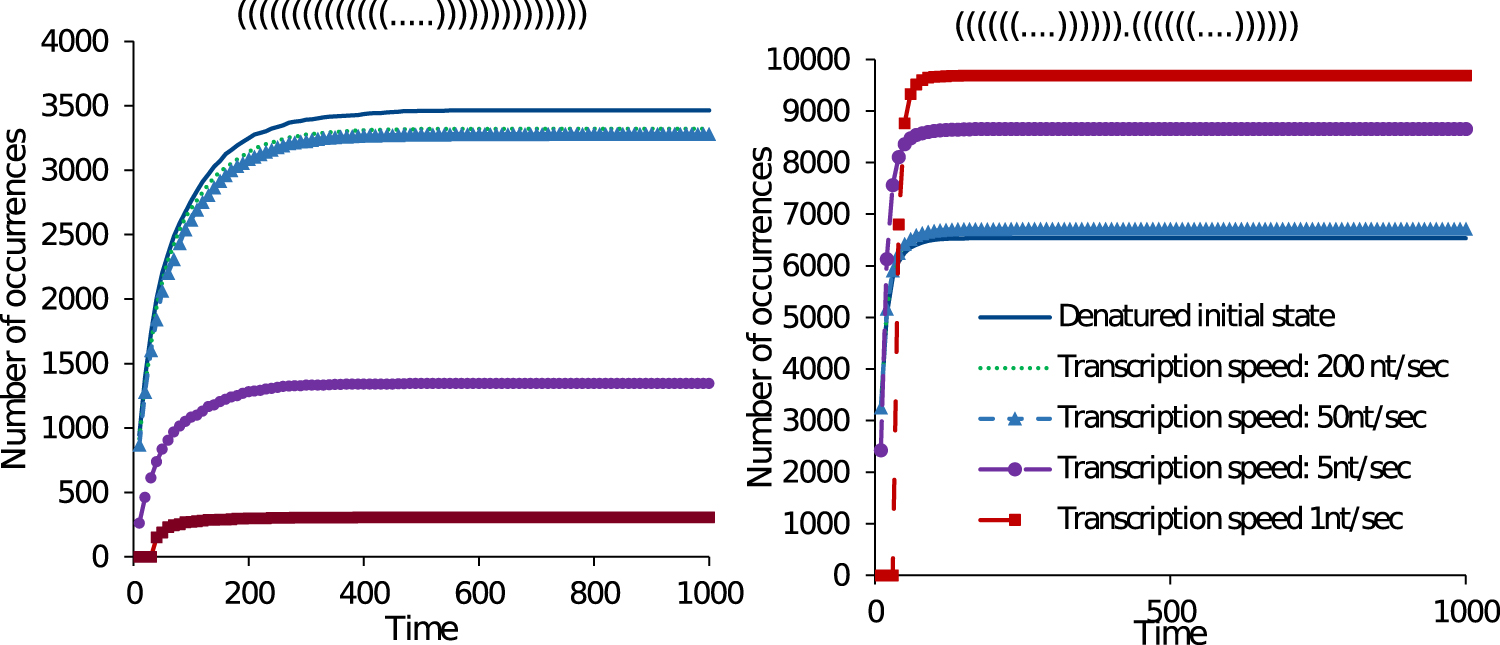
Figure 7 plots the number of first-hitting time occurrences of the MFE structure x and the suboptimal y with varying transcription speeds. We performed 10,000 simulation runs of the CoStochFold algorithm on the sequence S in which each simulation ran until a target structure was observed or the ending time $T_{m a x} = 1000$ seconds was reached. The constant $k_{0} = 1$ in Equation (2) is used in this case study to scale the time. Figure 7 shows that changing the transcription speed of the polymerase significantly affects the folding characteristics of the sequence. Specifically, cotranscriptional folding with slow transcription speed favors the suboptimal structure y. It increases the number of occurrences of y, while reducing the number of occurrences of the MFE structure x.

FIG. 7.

Cumulative first-hitting time occurrences of MFE structure x = “((((((((((((((.….))))))))))))))” (−26.20 kcal, left) and suboptimal y = “((((((.…)))))).((((((.…))))))” (−25.30 kcal, right). Time on the x-axis is in seconds of simulated time. MFE, minimum free energy.

Figure 8 compares the total number of first-hitting time occurrences of the MFE structure x with respect to the suboptimal conformation y up to time $T_{m a x} = 1000$ . We note that if the simulation starts from the fully denatured state, the occurrence ratio of the suboptimal conformation y to the MFE structure x is about 2:1, as also observed by Flamm et al. (2000). However, the ratio increases noticeably when the transcription speed decreases. For example, the occurrence ratio of the suboptimal conformation y to the MFE structure x is about 6.5:1 in the case of transcription speed 5 nt/s.

FIG. 8.

Total number of occurrences of MFE structure x = “((((((((((((((.….))))))))))))))” (−26.20 kcal) and suboptimal y = “((((((.…)))))).((((((.…))))))” (−25.30 kcal) with simulated time $T_{m a x} = 1000$ seconds by varying transcription speeds.

4.3. Beet soil-borne virus

We use the beet soil-borne virus S = “CGGUAGCGCGAACCGUUAUCGCGCA” from the PseudoBase++ database (Taufer et al., 2008) to demonstrate the application of our simulation in predicting RNA structures with pseudoknots. The folding of the sequence S was simulated with 10,000 runs. We evaluated the energy of pseudoknots using the energy parameters from Andronescu et al. (2010), which were estimated by fitting the standard NNDB parameters by Mathews et al. (1999) and pseudoknotted parameters by Dirks and Pierce (2003) over a large data set of both pseudoknotted and pseudoknot-free secondary structures. We compare two simulation settings: (1) cotranscriptional folding of S with transcription speed 200 nt/s and (2) the folding starting from the denatured initial state (i.e., a fully synthesized open strand). Figure 9 depicts the occurrence frequency of the H-type pseudoknotted structure C₁ = “.(((.[[[[[[)))…]]]]]].” with an energy of $- 12.39$ kcal. We also consider two intermediate structures C₂ = “.(((…[[[[)))…]]]]…” and C₃ = “.(((((.….…))))).….” having energies of $- 7.25$ and $- 4.52$ kcal, respectively.

FIG. 9.

Structural formation of the Beet soil-borne virus in (a) Cotranscription folding and (b) Folding from denatured initial state. Time on the x-axis is in seconds of simulated time.

Figure 9a and 9b clearly show that the dominant structure of the beet soil-borne virus sequence S is the H-type pseudoknotted structure C₁. We also observe from these figures that the folding starting from the denatured state misses the formation of intermediate structures C₂ and C₃, which appear in the cotranscriptional folding. After the transcription phase, intermediate structures will rearrange to C₁ and remain in this stable form. Figure 9a shows that the frequency of C₁ is >82% in the simulation.

We conclude this section with a note about the energy parameters for RNA structures with pseudoknots. In particular, we also simulated the beet soil-borne virus S with the energy model by Reidys et al. (2011), which is another extension of the NNDB model for pseudoknots. The occurrence frequency of pseudoknotted structure C₁ estimated by the Reidys et al. (2011) model was significantly lower than that by the Andronescu et al. (2010) model. This prediction discrepancy is because the energy model by Reidys et al. (2011) penalizes the formation of pseudoknots significantly more than the model by Andronescu et al. (2010). In fact, all pseudoknotted structures will be unfavorable with such high penalties for the pseudoknots. An interesting prediction from our cotranscriptional folding simulation using both energy models is the occurrence of the intermediate hairpin structure C₃. The persistence of C₃ before rearranging to the pseudoknot C₁ depends on how much penalty is applied to the formation of pseudoknots.

4.4. SV-11

SV-11 is a 115 nt long RNA sequence. It is a recombinant between the plus and minus strands of the natural Qβ template MNV-11 RNA (Biebricher and Luce, 1992). The result of the recombination is a highly palindromic sequence whose most stable secondary structure is a long hairpin-like structure, the MFE structure in Figure 10a. The MFE structure, however, disables Qβ replicase because its primer regions are blocked. Experimental work (Biebricher and Luce, 1992) has shown that an active structure of SV-11 for replication is when it folds into a metastable conformation depicted in Figure 10b. This is a hairpin–hairpin–multi-loop motif with open primer regions that serve as templates for replication. Transition from the metastable structure to the MFE structure has been observed experimentally but is rather slow (Biebricher and Luce, 1992), indicating long relaxation time to equilibrium.

FIG. 10.

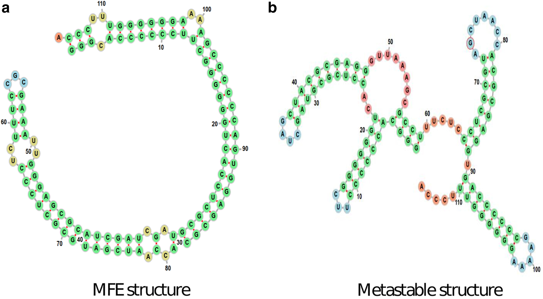
SV-11 with two conformations: (a) MFE structure (−95.90 kcal) and (b) metastable structure (−63.60 kcal). The visualization of structures is made by the Forna tool (Kerpedjiev et al., 2015).

We plot in Figure 11 the energy versus occurrence frequency of structures by the cotranscriptional folding of SV-11. The result is obtained by 10,000 simulation runs of our CoStochFold algorithm for t = 50 simulated seconds and average transcription speed 5 nt/s. To determine the frequency of occurrence of a structure, we discretize the simulation time into intervals and record how much time was spent in each structure within each interval. The frequency of occurrence of a structure in each time interval is then averaged over 10,000 runs. The figure shows that the folding favors metastable structures and disfavors the MFE structure. In particular, cotranscriptional folding quickly folds SV-11 to its metastable conformations with the mode of the energy distribution at about −63 kcal.

FIG. 11.

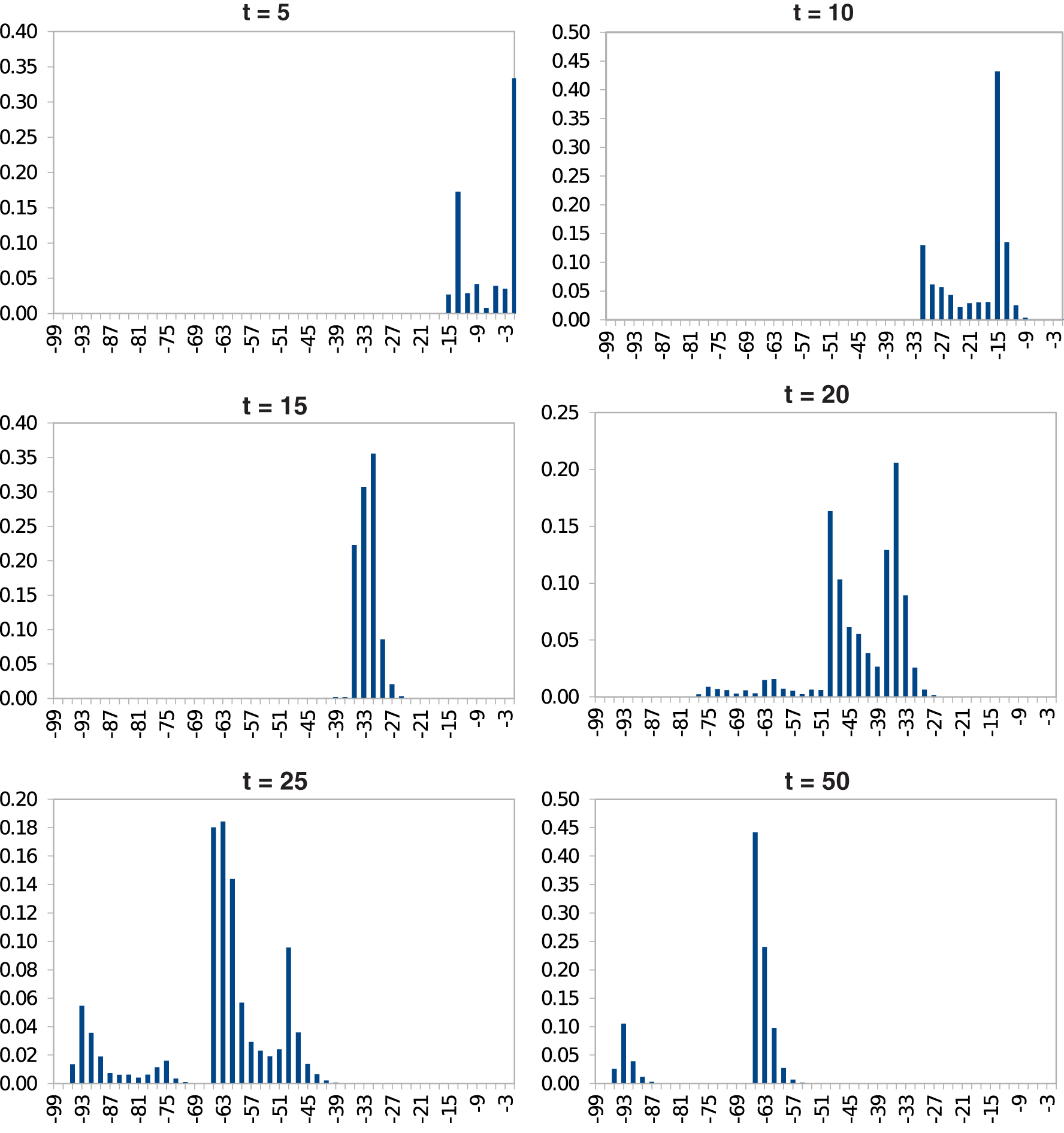
Cotranscriptional folding of SV-11. The x-axis denotes the energy level in kcal, and the y-axis shows the frequency of structures at a given energy level.

Figure 12 shows the long-term occurrence frequencies of structures at different energy levels in the SV-11-folding, and Figure 13 compares the occurrence frequencies of the specific metastable structure depicted in Figure 10b, with the MFE structure and two randomly selected suboptimal structures in the energy level of MFE structure. Figure 13 shows that the SV-11 molecule interestingly prefers the metastable structure over the MFE structure. Specifically, the metastable structure in the cotranscriptional folding regimen is in the time interval [0, 10,000] about 10-fold more frequent than the MFE structure.

FIG. 12.

Frequency of structures in folding SV-11.

FIG. 13.

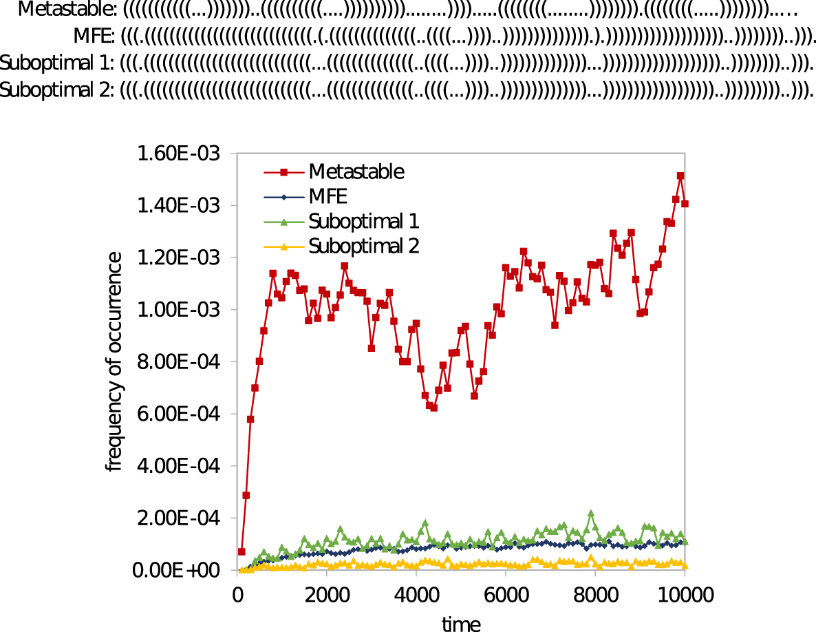
Frequency of the metastable structure in comparison with the MFE structure and two randomly selected suboptimal structures in the locality of the energy level of MFE.

4.5. Simulation performance

This section reports the performance of our stochastic folding algorithm with RNA sequences of varying lengths from 25 to 5000 nt. To estimate the computational cost of a single simulation move, we executed 10 independent simulation runs of 1000 simulation steps, each with a random sequence of the given length. The average runtime for each sequence length was computed and then divided by the number of simulation steps to assess the single-step computation cost.

Figure 14 plots the resulting estimated single-step computational cost of our folding algorithm in two settings: (1) simulation without pseudoknots, executed on Intel an i5-7300U dual-core CPU with a clock speed of 2.6 GHz, on the left and (2) simulation with pseudoknots, executed on an Intel i5-8365U quad-core CPU with a clock speed of 1.6 GHz, on the right. As witnessed by the figure, the simulation is quite computation intensive, especially for long sequences. For example, the simulation without pseudoknots for a sequence of length 1000 nt took on average 0.1 s of processor time per simulation step. Thus, a single simulation run of 1000 simulation steps would take on average 100 s, and 10,000 repeats of this would take 10⁶ s, that is, 11.6 days of processor time.

FIG. 14.

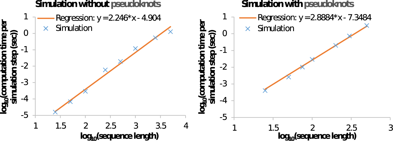
Computational runtimes of stochastic folding with sequences of varying lengths. Left: simulation without pseudoknots. Right: simulation with pseudoknots. Values on the x-axis and y-axis are in logarithmic scale.

The single-step computational cost increases with increasing sequence length: the runtime in the case of a pseudoknot-free simulation for sequences of length 5000 nt is about 11 times higher than for sequences of length 1000 nt. This increase is mostly due to the quadratically increasing number of possible moves in the locality of a conformation. Our detailed breakdown analysis of the computational cost of simulations shows that the cost of enumerating the possible moves contributes >95% of the total cost in each simulation step. (Note that the cost of enumerating the moves depends on both the number of possible moves and the algorithmics of the enumeration process.) The regression lines depicted in Figure 14 indicate that the computational cost per single move of our folding algorithm without pseudoknots grows as $O (N^{2.25})$ and with pseudoknots as $O (N^{2.89})$ , as a function of the sequence length N.

5. CONCLUSIONS

We propose a kinetic model of RNA folding that takes into account the elongation of an RNA chain during transcription as a primitive structure-forming operation alongside the common base pairing operations. We developed a new stochastic simulation algorithm CoStochFold to explore RNA structure formation, including pseudoknots, in the cotranscriptional folding regimen. We showed through numerical case studies that our method can quantitatively predict the formation of (metastable) conformations in an RNA folding pathway. The simulation method thus promises to offer useful insights into RNA folding kinetics in real biological systems. However, it also poses a great computational challenge for long sequences due to the huge number of possible moves in the locality of a conformation. Furthermore, many simulation runs must be performed to obtain a reasonable statistical estimation of the system dynamics. Several improvements are possible in future work. For instance, we can reduce the enumeration of possible moves by localizing the computation. The motif tree, a coarse-grained representation for pseudoknotted structures developed in the article, could be useful also in this context. We decompose an RNA structure into motifs and then enumerate new conformations related to each motif. To reduce the cost for executing many simulation runs, we can employ high-performance computing to run simulations in parallel.

Footnotes

AUTHOR DISCLOSURE STATEMENT

No competing financial interests exist.

FUNDING INFORMATION

This work has been supported by Academy of Finland grant no. 311639, “Algorithmic Designs for Biomolecular Nanostructures (ALBION).” The work of V.H.T. has been partially done when he was at Aalto University.

References

Akutsu

2000. Dynamic programming algorithms for RNA secondary structure prediction with pseudoknots. Discrete Appl. Math. 104, 45–62.

Al-Hashimi

H.M.

, and Walter

N.G.

2008. RNA dynamics: It is about time. Curr. Opin. Struct. Biol. 18, 321–329.

Andronescu

M.S.

, Pop

, and Condon

A.E.

2010. Improved free energy parameters for RNA pseudoknotted secondary structure prediction. RNA, 16, 26–42.

Biebricher

C.K.

, and Luce

1992. In vitro recombination and terminal elongation of RNA by Qβ replicase. EMBO J. 11, 5129–5135.

Bratsun

, Volfson

, Tsimring

L.S.

, et al. 2005. Delay-induced stochastic oscillations in gene regulation. PNAS, 102, 14593–14598.

Chen

H.-L.

, Condon

, and Jabbari

2009. An

O (n^{5})

algorithm for MFE prediction of kissing hairpins and 4-chains in nucleic acids. J. Comp. Biol. 16, 803–815.

Collins

L.J.

, and Penny

2009. The RNA infrastructure: Dark matter of the eukaryotic cell?. Trends Genet. 25, 120–128.

Dill

K.A.

1999. Polymer principles and protein folding. Protein Sci. 8, 1166–1180.

Dirks

R.M.

, and Pierce

N.A.

2003. A partition function algorithm for nucleic acid secondary structure including pseudoknots. J. Comp. Chem. 24, 1664–1677.

10.

Dykeman

E.C.

2015. An implementation of the Gillespie algorithm for RNA kinetics with logarithmic time update. Nucleic Acids Res. 43, 5708–5715.

11.

Fallmann

, Will

, Engelhardt

, et al. 2017. Recent advances in RNA folding. J. Biotechnol. 261, 97–104.

12.

Flamm

, Fontana

, Hofacker

I.L.

, et al. 2000. RNA folding at elementary step resolution. RNA, 6, 325–338.

13.

Gultyaev

A.P.

, van Batenburg

F.H.D.

, and Pleij

C.W.A.

1995. The computer simulation of RNA folding pathways using a genetic algorithm. J. Mol. Biol. 250, 37–51.

14.

Hofacker

I.L.

, Schuster

, and Stadler

P.F.

1998. Combinatorics of RNA secondary structures. Discrete Appl. Math. 88, 207–237.

15.

Hofacker

I.L.

, and Stadler

P.F.

2005. RNA secondary structures, 581–603. In Meyers, R.A., ed. Encyclopedia of Molecular Cell Biology and Molecular Medicine, Volume 12. Wiley-VCH Verlag GmbH, Weinheim, Germany.

16.

Hua

, Panja

, Wang

, et al. 2018. Mimicking co-transcriptional RNA folding using a superhelicase. J. Am. Chem. Soc. 140, 10067–10070.

17.

Isambert

, and Siggia

E.D.

2000. Modeling RNA folding paths with pseudoknots: Application to hepatitis delta virus ribozyme. PNAS, 97, 6515.

18.

Jasinski

, Haque

, Binzel

D.W.

, et al. 2017. Advancement of the emerging field of RNA nanotechnology. ACS Nano, 11, 1142–1164.

19.

Kawasaki

1966. Diffusion constants near the critical point for time-dependent Ising models. Phys. Rev. 145, 224–230.

20.

Kerpedjiev

, Hammer

, and Hofacker

I.L.

2015. Forna (force-directed RNA): Simple and effective online RNA secondary structure diagrams. Bioinformatics, 31, 3377–3379.

21.

Lai

, Proctor

J.R.

, and Meyer

I.M.

2013. On the importance of cotranscriptional RNA structure formation. RNA, 19, 1461–1473.

22.

Lyngsø

R.B.

, and Pedersen

C.N.S.

2000. RNA pseudoknot prediction in energy-based models. J. Comp. Biol. 7, 409–427.

23.

Marchetti

, Priami

, and Thanh

V.H.

2016. HRSSAefficient hybrid stochastic simulation for spatially homogeneous biochemical reaction networks. J. Comp. Phys. 317, 301–317.

24.

Marchetti

, Priami

, and Thanh

V.H.

2017. Simulation Algorithms for Computational Systems Biology. Springer, New York, NY.

25.

Mathews

D.H.

, Sabina

, Zuker

, et al. 1999. Expanded sequence dependence of thermodynamic parameters improves prediction of RNA secondary structure. J. Mol. Biol. 288, 911–940.

26.

Metropolis

, Rosenbluth

A.W.

, Rosenbluth

M.N.

, et al. 1953. Equation of state calculations by fast computing machines. J. Chem. Phys. 21, 1087–1092.

27.

Mironov

, and Kister

1986. RNA secondary structure formation during transcription. J. Biomol. Struct. Dynam. 4, 1–9.

28.

Mironov

A.A.

, and Lebedev

V.F.

1993. A kinetic model of RNA folding. Biosystems, 30, 49–56.

29.

Pan

, and Sosnick

T.R.

2006. RNA folding during transcription. Annu. Rev. Biophys. Biomol. Struct. 35, 161–175.

30.

Proctor

J.R.

, and Meyer

I.M.

2013. COFOLD: An RNA secondary structure prediction method that takes co-transcriptional folding into account. Nucleic Acids Res. 41, e102.

31.

Rastegari

, and Condon

2007. Parsing nucleic acid pseudoknotted secondary structure: Algorithm and applications. J Comput. Biol. 14, 16–32.

32.

Reeder

, and Giegerich

2004. Design, implementation and evaluation of a practical pseudoknot folding algorithm based on thermodynamics. BMC Bioinformatics, 5, 104.

33.

Reidys

C.M.

, Huang

F.W.D.

, Andersen

J.E.

, et al. 2011. Topology and prediction of RNA pseudoknots. Bioinformatics, 27, 1076–1085.

34.

Rivas

, and Eddy

S.R.

1999. A dynamic programming algorithm for RNA structure prediction including pseudoknots. J. Mol. Biol. 285, 2053–2068.

35.

Storz

2002. An expanding universe of noncoding RNAs. Science, 296, 1260–1263.

36.

Taufer

, Licon

, Araiza

, et al. 2008. PseudoBase++: An extension of PseudoBase for easy searching, formatting and visualization of pseudoknots. Nucleic Acids Res. 37, D127–D135.

37.

Thanh

V.H.

, Priami

, and Zunino

2014. Efficient rejection-based simulation of biochemical reactions with stochastic noise and delays. J. Chem. Phys. 141, 10B602.

38.

Thanh

V.H.

, and Zunino

2014. Adaptive tree-based search for stochastic simulation algorithm. Int. J. Comput. Biol. Drug. Des. 74, 341–357.

39.

Thanh

V.H.

, Zunino

, and Priami

2016. Efficient constant-time complexity algorithm for stochastic simulation of large reaction networks. IEEE/ACM Trans. Comput. Biol. Bioinform. 14, 657–667.

40.

Thanh

V.H.

, Zunino

, and Priami

2017. Efficient stochastic simulation of biochemical reactions with noise and delays. J. Chem. Phys. 146, 084107.

41.

Turner

D.H.

, and Mathews

D.H.

2009. NNDB: The nearest neighbor parameter database for predicting stability of nucleic acid secondary structure. Nucleic Acids Res. 38, D280–D282.

42.

Watters

K.E.

, Strobel

E.J.

, Yu

A.M.

, et al. 2016. Cotranscriptional folding of a riboswitch at nucleotide resolution. Nat. Struct. Mol. Biol. 23, 1124–1131.

43.

Zhao

, Zhang

, and Chen

S.-J.

2011. Cotranscriptional folding kinetics of ribonucleic acid secondary structure. J. Chem. Phys. 135, 245101.

44.

Zuker

1989. On finding all suboptimal foldings of an RNA molecule. Science, 244, 48–52.

45.

Zuker

, and Stiegler

1981. Optimal computer folding of large RNA sequences using thermodynamics and auxiliary information. Nucleic Acids Res. 9, 133–148.