RDscan: A New Method for Improving Germline and Somatic Variant Calling Based on Read Depth Distribution

Abstract

Several tools have been developed for calling variants from next-generation sequencing (NGS) data. Although they are generally accurate and reliable, most of them have room for improvement, especially regarding calling variants in datasets with low read depth. In addition, the somatic variants predicted by several somatic variant callers tend to have very low concordance rates. In this study, we developed a new method (RDscan) for improving germline and somatic variant calling in NGS data. RDscan removes misaligned reads, repositions reads, and calculates RDscore based on the read depth distribution. With RDscore, RDscan improves the precision of variant callers by removing false-positive variant calls. When we tested our new tool using the latest variant calling algorithms and data from the 1000 Genomes Project and Illumina's public datasets, accuracy was improved for most of the algorithms. After screening variants with RDscan, calling accuracies increased for germline variants in 11 of 12 cases and for somatic variants in 21 of 24 cases. RDscan is simple to use and can effectively remove false-positive variants while maintaining a low computation load. Therefore, RDscan, along with existing variant callers, should contribute to improvements in genome analysis.

1. Introduction

Over the past decade, large-scale sequencing of human genomes has been carried out using next-generation sequencing (NGS) technologies (Yi et al., 2010; The 1000 Genomes Project Consortium, 2015; Lek et al., 2016). Variants in human genomes are intimately associated with the genetic causes of many human diseases, as well as the genetic diversity within and among human populations (Ng et al., 2010; Lee et al., 2014). Therefore, identifying variants from NGS data has become a key foundation of human genome analysis.

The accuracy of variant calls for single-nucleotide variants (SNVs) and insertions and deletions (indels) depends on artifacts from sequencing device error, DNA contamination, and read misalignment (Li, 2014; Do and Dobrovic, 2015). These artifacts can lead variant callers to call artificial unreal variants. To minimize false-positive variant calling frequencies, several algorithms have been developed based on key features such as read depth, base/mapping quality, strand bias, and haplotype (DePristo et al., 2011; Garrison and Marth, 2012; Koboldt et al., 2013; Rimmer et al., 2014; Lai et al., 2016; Cho et al., 2018; Kim et al., 2018).

Recently, deep learning models such as DeepVariant (Poplin et al., 2018) and NeuSomatic (Sahraeian et al., 2019) have been implemented for variant calling based on these features. However, variant callers for the variants with low read depth and low variant allele frequency (VAF) still have room for improvement in terms of accuracy (Krøigård et al., 2016; Kim et al., 2018; Sahraeian et al., 2019).

To improve variant call accuracy, we propose read depth distribution as a new feature. We expect that the depth distribution of the aligned read set containing a variant should not differ from the depth distribution of the whole read set mapped to the same region, as genomic DNAs are randomly broken into smaller fragments and reads are generated from these fragments by NGS devices regardless of whether a variant is included (King et al., 2006). Hence, this similarity of the read depth distributions can be used to eliminate artificial variants; the variant candidate with read depth distribution similar to the overall read depth distribution should be kept as the true-positive variant, whereas other candidates should be removed as false. We used a similar approach for haplotyping the major histocompatibility complex regions (Ka et al., 2017).

In this study, we developed RDscan, a novel variant filtering method based on read depth distribution that effectively removes artificial variants. This method can improve the accuracy of variant calls relative to any other method. For most variant calling algorithms that we tested, the accuracies of these algorithms were further improved by differentiating real variants from false-positive variants using RDscan.

2. Materials and Methods

2.1. WGS data from public genome datasets

To evaluate the accuracy of RDscan for germline variants, we used WGS data for two samples, HG001 (34 × ) and HG002 (25 × ), from the 1000 Genomes Project (The 1000 Genomes Project Consortium, 2015); the detailed dataset information is provided in Supplementary Table S1. The reference standards, the Genome in a bottle (GIAB) truth sets for HG001 (v3.3.2) and HG002 (v4.1), were downloaded from ftp://ftp-trace.ncbi.nlm.nih.gov/giab/. The variant calling accuracy was evaluated within the high-confidence region suggested by GIAB.

2.2. In silico mixtures of unrelated germline samples

We used mixed DNA sequencing data from two unrelated individuals (NA12878 and NA12877) generated by Illumina (Kim et al., 2018) to evaluate the accuracy of somatic calls by RDscan. The dataset, consisting of three paired samples with different proportions of normal and tumor DNA purity (100% and 80%, 100% and 20%, and 90% and 80%), was downloaded from https://www.ncbi.nlm.nih.gov/sra/(Supplementary Table S1). The truth sets and the confidence region data for verification were downloaded from Illumina.

2.3. Collecting candidate variants

RDscan provides an additional filtering method for eliminating the false-positive variants called by the other variant callers. To collect the germline variants, we used GATK HaplotypeCaller (DePristo et al., 2011), Strelka2 (Kim et al., 2018), and DeepVariant (Poplin et al., 2018). For the somatic variants, we used Strelka2, VarDict (Lai et al., 2016), Mutect2 (Cibulskis et al., 2013), and NeuSomatic (Sahraeian et al., 2019). The collected variants are re-evaluated by the RDscan method, as described below.

2.4. Filtering misaligned reads in repeat region

RDscan prevents erroneous influence on variant calling by preliminarily removing misaligned reads in the repeat regions where one or more sequences appear more than three times repeatedly. Specifically, a read that starts or ends in a repeat region is considered misaligned. As an example, shown in Step 2 of Figure 1, a repeat region consists of nucleotide sequences that repeat TG four times.

FIG. 1.

Overview of RDscan based on read depth distribution. The workflow of RDscan is summarized in six steps. In Step 1, a variant caller produces a VCF file of candidate variants. Among the candidate variants, this figure deals with AT deletion variants occurring at locus i. For the reads mapped to locus i, in Step 2, RDscan filters the misaligned reads to ensure call accuracy. Reads that start or end in a repeat region are considered misaligned. In this example, the repeat region consists of a nucleotide sequence that repeats TG four times, and the top four reads and the bottom read are removed. In Step 3, all remaining reads are tagged as ALL, and all the reads containing the variant are tagged as VAR. If the variant is an indel, as shown in Step 4, RDscan adjusts the read alignment to eliminate alignment region length differences between ALL and VAR. Finally, in Step 5, RDscan estimates the RDscore for the AT deletion variant, which represents the correlation depths of ALL and VAR in the Comparison Region. The Comparison Region is the area in which the reads in ALL are aligned. For each candidate variant, the estimated RDscore is recorded in the original VCF file through iterations of Steps 2 through 5. VCF, Variant Call Format.

In this case, we can simultaneously observe two variations at locus i, one for having G instead of the reference sequence A, and the other for the AT deletion. However, the top four reads with their ends in the repeat region cannot differentiate the case of variation G from the case of AT deletion because they do not have sequence information to anchor after the repeat region. For reads extending beyond the repeat region, the sequence alignment before and after the repeat region will force the variant to be either G or deletion of AT; otherwise, the misidentification would lead to a positional shift of the sequences after the repeat region. Hence, if the start or end of a read is aligned in a repeat region, we consider the read as having a risk of misalignment, and therefore eliminate it.

2.5. A new variant calling method

In this section, we introduce a new method for determining the reliability of a variant call by comparing the read depth distribution with the variant to the whole read depth distribution aligned over the variant locus. For each candidate variant, RDscan first extracts all reads aligned to the locus of the variant in the corresponding Binary Alignment Map (BAM) file, and then removes misaligned reads in the repeat regions, as described in the previous section. This set of filtered reads is called ALL. Among the reads in ALL, RDscan extracts VAR, a new set of reads containing the variant (Step 3 in Fig. 1). If the variant is an indel, it causes a difference in the aligned area lengths of reads between ALL and VAR, which adversely affects the calculation of the correlation of the read depth distribution between the two groups.

To prevent this, RDscan adjusts alignment of the reads. As shown in Step 4 of Figure 1, the reads with the AT deletion have an aligned region longer than other reads by the length of the deleted sequence. In this example, RDscan decreases the aligned area of the reads with the AT deletion by the length of the deletion. Conversely, in the case of an insertion variant, the aligned region is increased by the length of the variant. To compare the read depth distributions between ALL and VAR, RDscan calculates the read depths for each group.

We denote the read depth of the group X at locus i as $D_{X}^{i}$ and the read depth vector of the group X as $D_{X} = [D_{X}^{s l}, D_{X}^{s l + 1}, \dots, D_{X}^{s l + l - 1}]$ , where sl is the start locus of the Comparison Region and l is the length of the region. The Comparison Region is the area in which the reads in ALL are aligned. RDscan then uses the following score function to determine the reliability of the variant:

The RDscore ranges from 0 to 1. The RDscore of a variant ∼1 indicates that the variant is reliable. We used ALGLIB library (ALGLIB; https://www.alglib.net/) to calculate the Pearson correlation coefficient (corr) between the depths of ALL and VAR. The exponent value at Eq. (1) is to maximize the difference between the corrs of true-positive and false-positive variants. Specifically, the reference corr for the true-positive variants was set to 0.86, which preserves a sensitivity of 95% and 99.9% for NA12878 sample with coverage of 34 × and 300 × , respectively (Fig. 2).

FIG. 2.

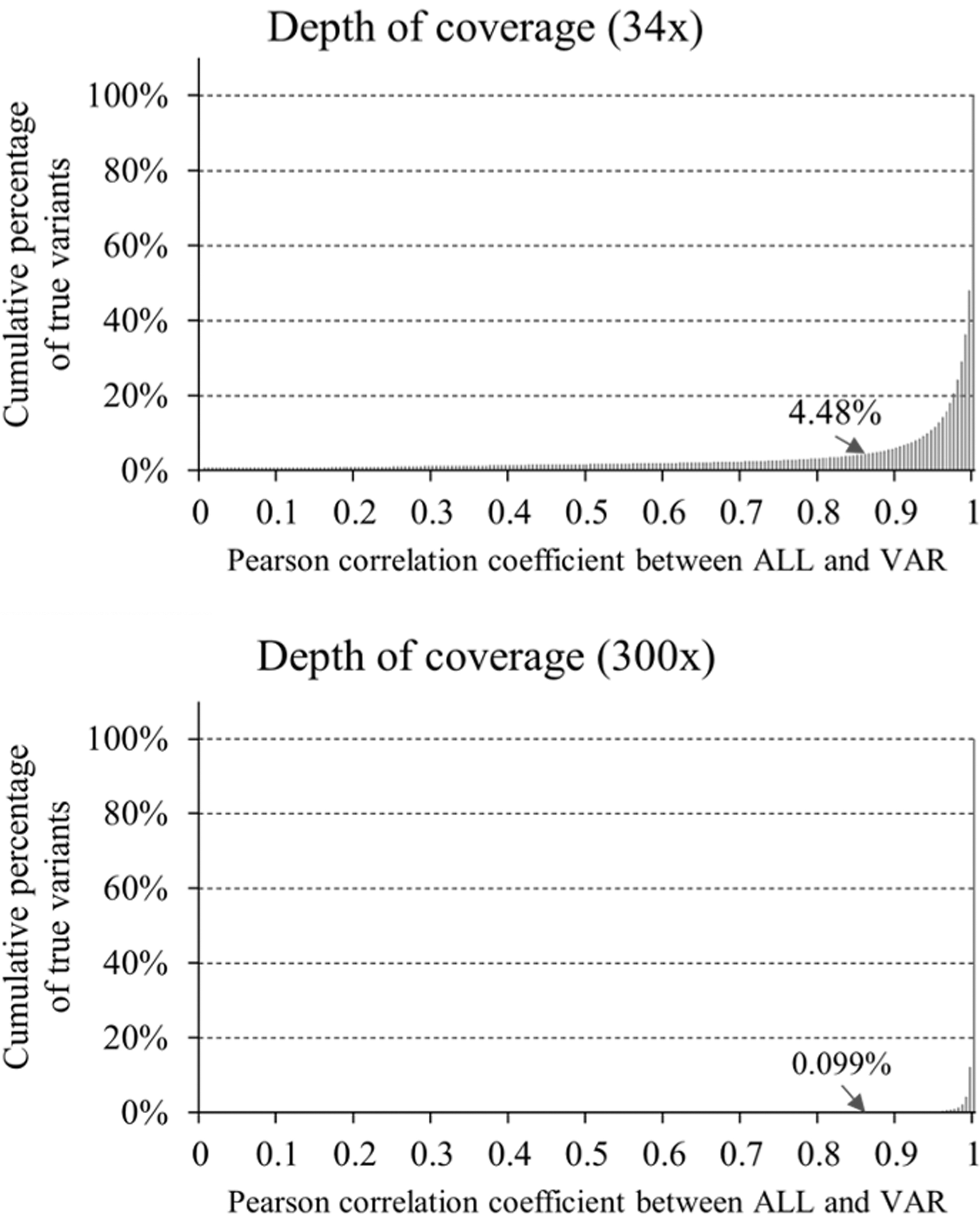
The cumulative distributions of the Pearson correlation coefficients between ALL and VAR of the true-positive variants (3,544,295) within the two NGS data with coverage of 34 × and 300 × for the NA12878 sample. NGS, next-generation sequencing.

The reference corr of false-positive variants was set from the average corr of the false-positive variants from each algorithm. For the NA12878 sample with coverage of 34 × , the average corrs of the false-positive variants were 0.231, 0.431, and 0.245 for Strelka2, GATK Haplotype Caller, and DeepVariant, respectively. The exponent values of the Rdscore, which maximize the distance between the reference corrs of true-positive and false-positive variants, are 1.7, 2.5, and 1.8, respectively. As a result, the average (2.0) of those values is used for the exponent value.

2.6. Variant calling method from paired tumor and normal samples

A variant that is present in a cancerous tissue, but not in matched normal tissue, is called a somatic variant. In practice, the normal sample may contain some tumor cells, or the tumor sample could be contaminated by normal cells; either case could cause real somatic variants to be discarded. To address this problem, RDscan considers the VAF of the tumor and normal samples. First, RDscan calculates the RDscores (RD_tumor and RD_normal) of a variant from the tumor and matched normal samples, respectively, using Eq. (1) in the previous section. Then, RDscan uses the following score function to determine whether the variant is somatic:

The possible range of the RDscore_somatic is 0–1 for a variant; a score ∼1 means that the variant is somatic variant. For a given variant, VAF_tumor and VAF_normal represent, respectively, the variant allele frequencies of tumor and normal tissues.

3. Results

3.1. Evaluations of germline variant calling accuracy

We ran RDscan with candidate variant sets from three germline variant callers (Strelka2, GATK HaplotypeCaller, DeepVariant) using two public datasets (HG001 and HG002). Germline variant callers were executed based on the best practices described by the authors (Supplementary Table S2). Germline variant calling accuracy was evaluated using “hap.py” (Krusche et al., 2019) relative to the GIAB truth set. In this study, we assumed that germline variants with RDscore > 0.5 were true-positive variants.

We first compared the original set of variants called by each algorithm with the variants subjected to further filtering with RDscan. The original set of variants consisted of variants that passed all filtering criteria provided by each variant caller. Overall, RDscan improved variant calling accuracy by decreasing the number of false-positive calls (FPs) while minimizing the reduction in true-positive calls (TPs). As shown in Table 1, for SNVs in HG001, the number of FPs was reduced by 69.5% for Strelka2 (from 438,358 to 133,573), 54.1% for GATK HaplotypeCaller (139,993 to 64,219), and 36.0% for DeepVariant (from 115,512 to 73,911), whereas the numbers of TPs were reduced by 0.65%, 0.74%, and 0.72%, respectively. After screening with RDscan, the accuracy (F-score) for SNVs was higher in all six cases, and the accuracy for indels was higher in five of six cases.

Table 1.

Germline Variant Calling Accuracy

Dataset	Variant caller	Filter	SNVs						Indels
Dataset	Variant caller	Filter	True positive	False positive	False negative	Rec. (%)	Pre. (%)	F-scr. (%)	True positive	False positive	False negative	Rec. (%)	Pre. (%)	F-scr. (%)
HG001 (34 × )	Strelka2 v2.9.10	PASS	2,900,173	438,358	309,142	90.4	86.9	88.6	359,961	145,261	121,879	74.7	71.2	72.9
	Strelka2 v2.9.10	PASS+RD	2,881,124	133,573	328,191	89.8	95.6	92.6	349,426	122,261	132,414	72.5	74.1	73.3
	GATK HaplotypeCaller v4.1.8.1	PASS	3,118,927	139,993	90,388	97.2	95.7	96.4	342,216	219,032	139,624	71.0	61.0	65.6
	GATK HaplotypeCaller v4.1.8.1	PASS+RD	3,095,699	64,219	113,616	96.5	98.0	97.2	331,283	155,762	150,557	68.8	68.0	68.4
	DeepVariant v1.0.0	PASS	3,112,316	115,512	96,999	97.0	96.4	96.7	369,765	196,180	112,075	76.7	65.3	70.6
	DeepVariant v1.0.0	PASS+RD	3,089,778	73,911	119,537	96.3	97.7	97.0	360,009	155,192	121,831	74.7	69.9	72.2
HG002 (25 × )	Strelka2 v2.9.10	PASS	2,788,428	727,723	564,390	83.2	79.3	81.2	319,335	52,059	203,699	61.1	86.0	71.4
	Strelka2 v2.9.10	PASS+RD	2,759,569	252,484	593,249	82.3	91.6	86.7	310,899	452,31	212,135	59.4	87.3	70.7
	GATK HaplotypeCaller v4.1.8.1	PASS	3,094,172	256,578	258,646	92.3	92.3	92.3	324,496	180,164	198,538	62.0	64.3	63.2
	GATK HaplotypeCaller v4.1.8.1	PASS+RD	3,057,662	123,573	295,156	91.2	96.1	93.6	310,722	117,435	212,312	59.4	72.6	65.3
	DeepVariant v1.0.0	PASS	3,117,943	227,805	234,875	93.0	93.2	93.1	358,205	152,505	164,829	68.5	70.1	69.3
	DeepVariant v1.0.0	PASS+RD	3,082,064	150,850	270,754	91.9	95.3	93.6	345,302	120,230	1,77,732	66.0	74.2	69.9

Recall, precision, and F-score are expressed as Rec., Pre., and F-scr., respectively. PASS is the set of variants that passed all filtering criteria provided by each variant caller, and PASS+RD is the set of variants in PASS that passed additional filtering with RDscan. F-scores are calculated by the following equation: $2 \times \frac{(p r e c i s i o n \times r e c a l l)}{(p r e c i s i o n + r e c a l l)}$ . Bold font indicates that the accuracy of the variants selected by RDscan is higher than the original accuracy of each algorithm.

indels, insertions and deletions; SNVs, single-nucleotide variants.

We also show the overall improvement in the performance of these algorithms achieved by RDscan. As shown in Figure 3, performance for indels was noticeably improved, whereas for SNVs RDscan slightly improved the variant calling performance relative to DeepVariant, even though it already had excellent variant calling accuracy. For both datasets, the overall performance of these three algorithms was improved when the variants were screened by RDscan (Supplementary Fig. S1).

FIG. 3.

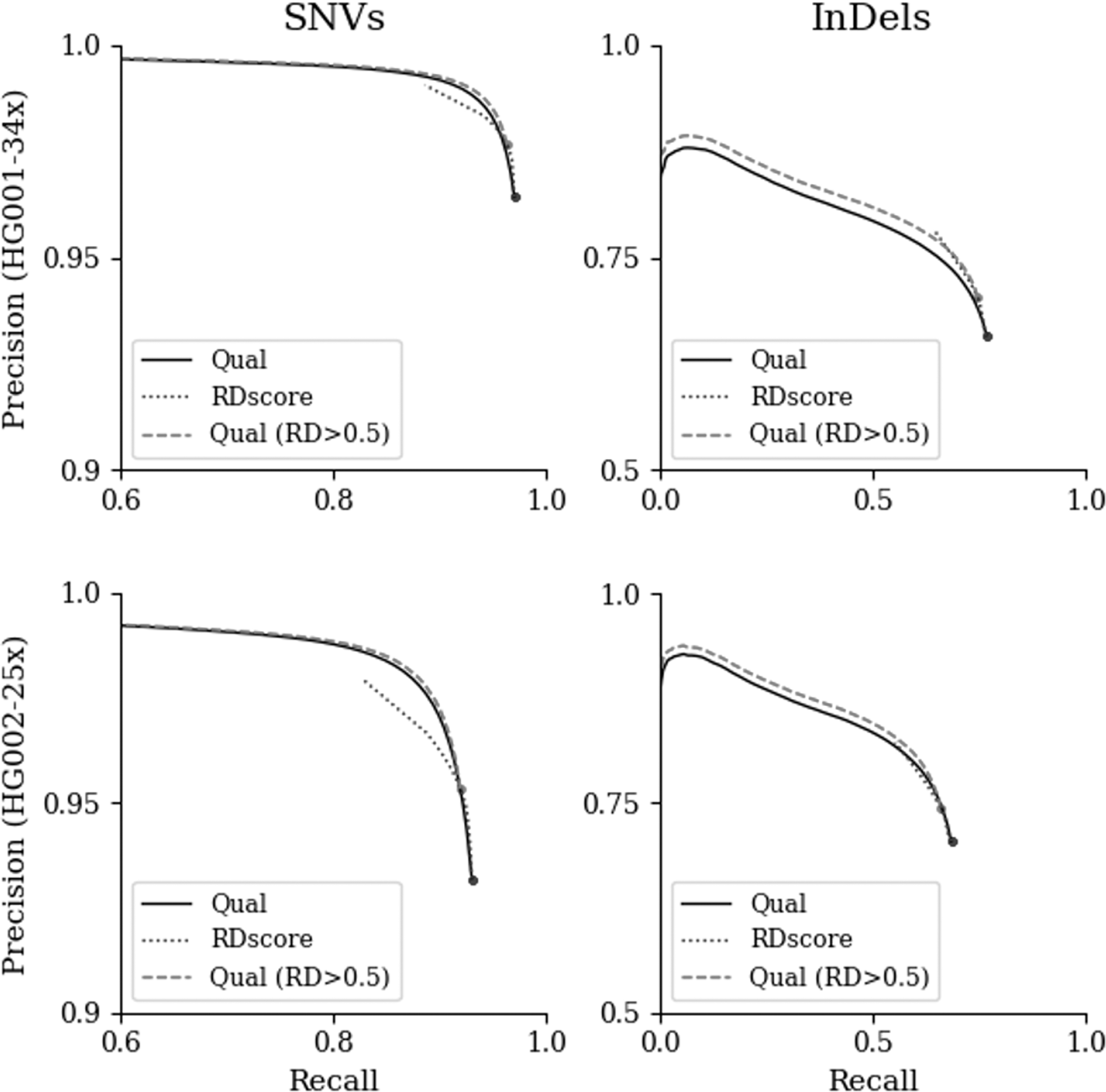
Variant calling accuracy changes according to DeepVariant and RDscan scores. For two datasets (HG001 and HG002), the Receiver Operating Characteristic (ROC) curve shows the variation in recall and precision of the variant call with a scoring parameter. The scoring parameters used to generate the solid and dotted curves were Qual (DeepVariant) and RDscore (RDscan), respectively. The dashed lines, Qual (RD >0.5), show the results of applying RDscore > 0.5 to the sets of variants according to the Qual parameter of DeepVariant (solid line).

The additional burden of the quality checks should be relatively moderate. RDscan is simple to use and can effectively remove false-positive variants while still having a low computation load (∼2 hours using Intel Xeon E5620 2.4 GHz, 12 cores, and 64 GB memory for one WGS dataset) relative to the runtime of the entire variant call pipeline. The memory usage requirement for RDscan is 5–10 GB.

3.2. Evaluations of somatic variant calling accuracy for paired tumor and normal samples

Next, we evaluated the performance of RDscan for somatic variant calling using in silico mixed datasets and the truth set provided by Illumina (Kim et al., 2018). We used these data to run some of the known somatic variant callers (Strelka2, VarDict, Mutect2, and NeuSomatic), and then ran RDscan to further screen the results obtained with each caller. The somatic variant callers were executed using the best practices provided by the authors (Supplementary Table S2). We first tried running the latest version (v4.1.8.1) of Mutect2 using the best practice pipeline provided by bcbio-nextgen (Chapman et al., 2021).

This pipeline includes the step of removing known germline variants by reference to an external database. Consequently, higher somatic variant calling accuracy is expected for a typical Tumor-Normal dataset. However, for the in silico datasets generated based on the germline variants used for verification in this article, most of the variants were filtered out by this method, making analysis impossible. Therefore, we used Mutect2 (v4.1.1.0) as an alternative method to proceed only with basic somatic variant calling from the in silico datasets. We used “som.py” (Krusche et al., 2019) to evaluate somatic variant calling accuracy against the in silico germline mixture truth sets. In this study, variants with RDscore_somatic > 0.3 were considered true-positive somatic variants.

We first compared the original variants of the algorithms with the variants selected by RDscan. The original set of variants consisted of variants that passed all filtering criteria provided by each variant caller. Overall, variant calling accuracies of four algorithms were improved after the variants were screened using RDscan. As shown in Table 2, after screening with RDscan, the call accuracies for SNVs increased in 10 of 12 cases, and the call accuracies for indels increased in 11 of 12 cases.

Table 2.

Somatic Variant Calling Accuracy

Dataset	Variant caller	Filter	SNVs						Indels
Dataset	Variant caller	Filter	True positive	False positive	False negative	Rec. (%)	Pre. (%)	F-scr. (%)	True positive	False positive	False negative	Rec. (%)	Pre. (%)	F-scr. (%)
Tumor 20% (∼110 × ) Normal 100% (∼37 × )	Strelka2 v2.9.10	PASS	1,092,894	26,851	173,792	86.3	97.6	91.6	102,895	9830	100,818	50.5	91.3	65.0
	Strelka2 v2.9.10	PASS+RD	1,078,316	21,521	188,370	85.1	98.0	91.1	101,324	8869	102,389	49.7	92.0	64.6
	VarDict v1.8.2	PASS	688,675	16,065	578,011	54.4	97.7	69.9	46,866	8372	156,847	23.0	84.8	36.2
	VarDict v1.8.2	PASS+RD	687,062	11,124	579,624	54.2	98.4	69.9	46,447	2872	157,266	22.8	94.2	36.7
	NeuSomatic v0.2.1	PASS	976,872	12,082	289,814	77.1	98.8	86.6	52,349	3079	151,364	25.7	94.4	40.4
	NeuSomatic v0.2.1	PASS+RD	971,781	11,180	294,905	76.7	98.9	86.4	52,020	1132	151,693	25.5	97.9	40.5
	Mutect2 v4.1.1.0	PASS	1,167,087	147,578	99,599	92.1	88.8	90.4	166,506	132,258	37,207	81.7	55.7	66.3
	Mutect2 v4.1.1.0	PASS+RD	1,150,492	64,552	116,194	90.8	94.7	92.7	154,366	51,034	49,347	75.8	75.2	75.5
Tumor 80% (∼110 × ) Normal 100% (∼37 × )	Strelka2 v2.9.10	PASS	1,221,652	60,742	45,034	96.4	95.3	95.9	167,249	34,894	36,464	82.1	82.7	82.4
	Strelka2 v2.9.10	PASS+RD	1,221,070	54,032	45,616	96.4	95.8	96.1	166,715	32,429	36,998	81.8	83.7	82.8
	VarDict v1.8.2	PASS	1,099,023	33,498	167,663	86.8	97.0	91.6	97,715	29,101	105,998	48.0	77.1	59.1
	VarDict v1.8.2	PASS+RD	1,098,606	26,965	168,080	86.7	97.6	91.8	97,419	22,277	106,294	47.8	81.4	60.2
	NeuSomatic v0.2.1	PASS	1,183,322	42,631	83,364	93.4	96.5	94.9	97,764	14,630	105,949	48.0	87.0	61.9
	NeuSomatic v0.2.1	PASS+RD	1,182,991	32,205	83,695	93.4	97.3	95.3	97,740	7210	105,973	48.0	93.1	63.3
	Mutect2 v4.1.1.0	PASS	1,194,772	59,587	71,914	94.3	95.2	94.8	171,710	83,012	32,003	84.3	67.4	74.9
	Mutect2 v4.1.1.0	PASS+RD	1,194,272	46,224	72,414	94.3	96.3	95.3	168,325	55,815	35,388	82.6	75.1	78.7
Tumor 80% (∼110 × ) Normal 90% (∼37 × )	Strelka2 v2.9.10	PASS	1,079,088	44,545	187,598	85.2	96.0	90.3	105,880	18,254	97,833	52.0	85.3	64.6
	Strelka2 v2.9.10	PASS+RD	1,078,587	38,544	188,099	85.2	96.5	90.5	105,528	16,695	98,185	51.8	86.3	64.8
	VarDict v1.8.2	PASS	485,305	22,976	781,381	38.3	95.5	54.7	47,676	18,266	156,037	23.4	72.3	35.4
	VarDict v1.8.2	PASS+RD	484,945	16,619	781,741	38.3	96.7	54.9	47,401	11,399	156,312	23.3	80.6	36.1
	NeuSomatic v0.2.1	PASS	1,016,718	59,879	249,968	80.3	94.4	86.8	61,454	6590	142,259	30.2	90.3	45.2
	NeuSomatic v0.2.1	PASS+RD	1,016,460	21,555	250,226	80.2	97.9	88.2	61,439	3102	142,274	30.2	95.2	45.8
	Mutect2 v4.1.1.0	PASS	584,814	30,393	681,872	46.2	95.1	62.2	98,159	43,597	105,554	48.2	69.2	56.8
	Mutect2 v4.1.1.0	PASS+RD	584,480	22,219	682,206	46.1	96.3	62.4	96,282	28,482	107,431	47.3	77.2	58.6

Table 2 also shows that most variant callers had difficulty in producing high-accuracy results from samples with low-tumor purity. In the case of SNVs, the F-score of the samples with low-tumor purity (T:20%, N:100%) decreased by 3.9% for Strelka2, 15.9% for VarDict, 7% for NeuSomatic, and 4.6% for Mutect2 relative to samples with high-tumor purity (T:80%, N:100%). Despite the difficulties of variant calling in samples with low-tumor purity, RDscan achieved consistent improvement in accuracy over the variant callers we tested. In addition, even with normal samples contaminated by tumor cells (T:80%, N:90%), RDscan improved the accuracy of the variant callers.

Second, to show the overall improvement in the performance of these algorithms achieved by RDscan, we compared the changes in precision and recall of the variants according to the score of each algorithm with the changes resulting from application of RDscan to those variants. As shown in Figure 4, for both SNVs and indels, RDscan improved the performance of the variant calls from Strelka2. For all three datasets, the overall performance of these four algorithms was improved when the variants were screened with RDscan (Supplementary Fig. S2).

FIG. 4.

Changes in somatic variant calling accuracy according to Strelka2 and RDscan scores. For three datasets, ROC curve shows the change of recall and precision for the variant calls according to a scoring parameter. The scoring parameters used to generate the solid and dotted curves were SomaticEVS (Strelka2) and RDscore (RDscan), respectively. The dashed lines, SomaticEVS (RD >0.3), show the results of applying RDscore_somatic > 0.3 for the sets of variants according to SomaticEVS of Strelka2 (solid line).

3.3. Somatic variant calling accuracy of ensemble models

To compare RDscan with the same level methods, the results of using the well-known variant callers as filters were compared with the results of RDscan. We analyzed the accuracies of ensemble models that combined two somatic variant calling algorithms (one as a variant caller and the other as a filter). Six ensemble models were created by combining the four algorithms. For each model with two algorithms, we generated a set of variants that passed the default criteria of both algorithms’ filters, and then evaluated them.

We compared 14 results from six ensemble models, four existing algorithms, and four models analyzed with RDscan. Figure 5 shows the top three results for each dataset, in order of accuracy. In the case of SNVs, the combination of Strelka2 and RDscan had the highest accuracy in the two datasets with 80% tumor purity, and the combination of Mutect2 and RDscan had the highest accuracy in the dataset with 20% tumor purity. Indels exhibited similar results to SNVs, but in the case of the dataset with 80% tumor and 100% normal purity, the combination of Mutect2 and Strelka2 had the best accuracy, and the combination of Strelka2 and RDscan had the second highest accuracy.

FIG. 5.

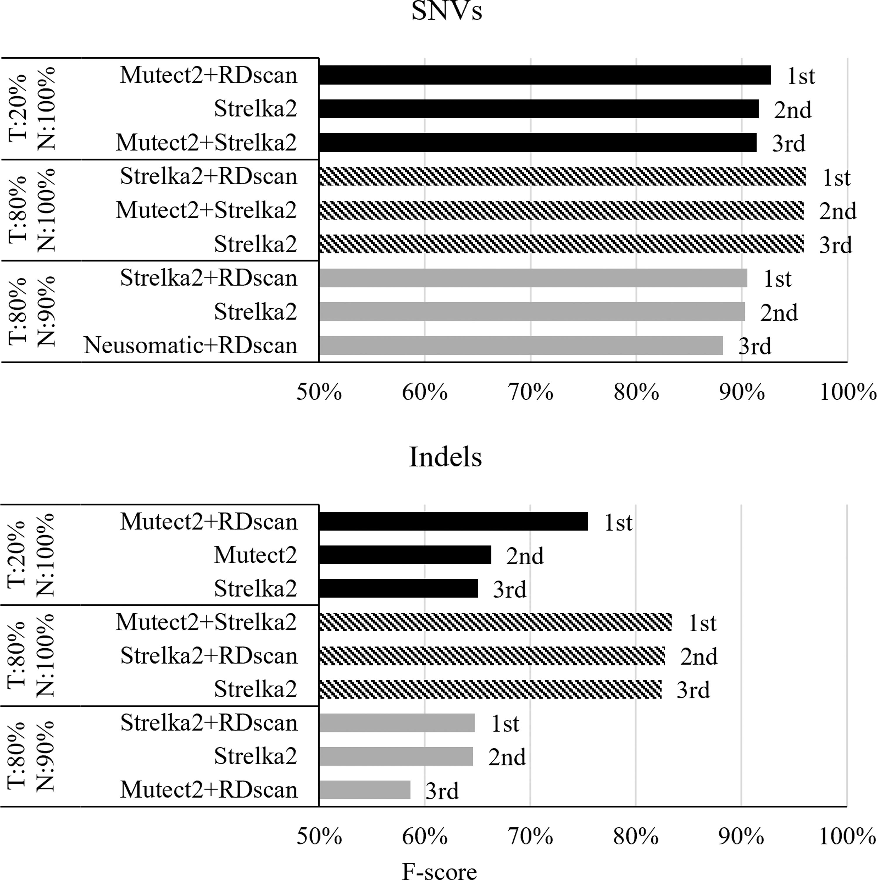
Somatic variant calling accuracies of ensemble models. To evaluate the performance of ensemble models, 14 models (6 ensemble models, 4 models analyzed with RDscan, and 4 existing algorithms) were used along with three datasets with proportions of tumor and normal DNA purity of 20% and 100%, 80% and 100%, and 80% and 90%. This figure shows the top three models in order of SNV/indels call accuracy for each dataset. Indels, insertions and deletions; SNV, single-nucleotide variant.

Note that RDscan effectively removes artificial variants, significantly improving variant call accuracy for indels in samples with low-tumor purity, where it is difficult to distinguish true variants from artificial variants. The results for all models are shown in Supplementary Table S3.

3.4. Relationship between read depth coverage, indel length, RDscore, and variant calling accuracy

There are several parameters that influence call accuracy. The major factor would be depth coverage. The depth ranges of the current main technology are 30–70 × for WGS and 100–150 × for whole-exome sequence. To assess the accuracy of RDscan as a function of depth coverage, we ran RDscan with candidate variant sets from the three germline variant callers using an additional dataset, HG002 (300 × ), with high depth coverage. Similar to the analysis in the previous section, we compared the original set of variants called and passed by each algorithm with the variants further filtered by RDscan. Supplementary Table S4 shows that additional screening with RDscan is ineffective for datasets with a high depth coverage. We will address this issue in the Discussion section.

RDscan assumes that the depth distribution of the aligned read set containing a variant should not differ from the depth distribution of the whole read set mapped to the same region. However, the two distributions could be different for a long indel, because the sequencing quality and mapping quality scores of sequence reads with long indels may be lower than those of sequence reads without variants.

To evaluate the RDscore changes according to an indel length, we calculated the RDscores of all heterozygous indels in the GIAB truth sets. Among the 263,034 indels, we analyzed 220,097 indels with at least one sequence read in the HG001 (34 × ) BAM file. Supplementary Figure S3 shows that the RDscore slightly decreases as the length of indel increases. However, the medians of the RDscores are between 0.8 and 1.0 for all indel lengths, which can be distinguished from artificial variants (in this study, we assumed that germline variants with RDscore < 0.5 were artificial variants).

4. Discussion

Numerous methods have been developed for detecting variants from NGS data. Although the existing variant calling algorithms are generally accurate and reliable, most of them still have room for improvement in terms of accuracy for the variants with low VAF. RDscan removes misaligned reads and repositions reads, and then calculates RDscore based on the read depth distribution. By adopting this score, the accuracy of SNV/indel calls can be improved relative to the results obtained using existing variant callers.

Although RDscan can improve variant calling accuracy in most cases, it is important to use it with an understanding of the characteristics of RDscore. First, the RDscores of the true-positive variants are very densely distributed over a particular value. For example, 98.65% (3,076,963 of 3,118,927) of the true-positive variants called by GATK HaplotypeCaller for SNVs have RDscore > 0.64. Because variants with RDscore > 0.64 already have very high reliability in terms of the correlation (>0.8) of read depth distribution, variant filtering using RDscore > 0.64 can decrease the sensitivity of variant calls. Second, variant filtering with low RDscore increases the variant call precision while minimizing the reduction in sensitivity.

In particular, in the case of somatic variants in Figure 4, precision increases rapidly as RDscore increases (blue dots mean RDscore = 0, red dots mean RDscore = 0.3). Even with a loose RDscore criterion, RDscan can find many false calls not identified by existing methods. In this study, we used RDscore criteria of 0.5 and 0.3 for germline and somatic variants, respectively. The RDscore ranges from 0 to 1, but we recommend using an RDscore <0.64.

Third, Supplementary Table S4 shows that although RDscan can still increase the precision of variant calls, there is little room for precision improvement, resulting in a slightly decrease in the variant call accuracy for deep sequencing data. For example, the precision values of DeepVariant's SNV and indels calls were already very high, at 99.88% and 99.82%, respectively. Therefore, we recommend using RDscan for typical sequencing data with relatively low read depth coverage, rather than for deep sequencing data.

In the last decade, many algorithms have been introduced to achieve high performance using features of NGS data such as read depth, base and mapping quality score, strand bias, and haplotype. In this article, we propose a new feature, read depth distribution. To validate the effectiveness of the read distribution, we first developed our own variant caller (standalone) based on read depth distribution. The accuracy of the variant caller was comparable with, but not better than, the state-of-art variant callers. However, we demonstrated that read depth distribution can increase the accuracy of variant calls when used with other features. Read depth distribution can be used as a key feature of genomic analysis, along with the existing NGS data features.

5. Conclusion

RDscan is an SNV/indels filtering tool based on the read depth distribution of an NGS dataset. In this study, we showed that our method could improve the accuracy of germline and somatic variant calls from NGS data. In addition, RDscan is simple to use and can effectively remove false-positive variants while maintaining a low computation load. Therefore, RDscan, along with existing variant callers, will contribute to improvement in genome analysis. Future work should seek to develop new methods based on read depth distribution for sequence analysis other than variant calling and haplotyping.

Footnotes

Authors’ Contributions

S.L. contributed to conceptualization; methodology; software; writing—original draft; and writing—review and editing. S.H. contributed to software; visualization; writing—original draft; and writing—review and editing. J.W. and J.-H.L. performed formal analysis; writing—original draft. K.K. performed data curation and formal analysis. L.K. contributed to conceptualization and resources. K.P. provided conceptualization and methodology. J.J. contributed to conceptualization, methodology, and supervision.

Availability of Data and Implementation

Source code and binaries, implemented in C++ and supported on Linux, are freely available for download at https://github.com/satchellhong/RDscan. The sequencing data for HG001-HG002 and in silico mixtures used in this study are obtained from the 1000 Genomes Project (www.internationalgenome.org/) and the National Center for Biotechnology Information (NCBI, https://www.ncbi.nlm.nih.gov/), respectively. Detailed descriptions about the data can be found in .

Acknowledgments

The authors thank all members of the Precision Medicine Support Center at Inha University Hospital for their generous support in testing the NGS data.

Author Disclosure Statement

The authors declare they have no competing financial interests.

Funding Information

This research was supported in part by Basic Science Research Program through the National Research Foundation of Korea (NRF) funded by the Ministry of Science and ICT (NRF-2019M3E5D4064683). K. Park was supported by NRF-2014M3C9A3063541.

Supplementary Materials

References

Chapman

, Kirchner

.; Pantano

, et al. 2021. bcbio/bcbio-nextgen. Available at: https://github.com/bcbio/bcbio-nextgen. Accessed October 21, 2020.

Cho

, Lee

, Hong

J.H.

, et al. 2018. Development of the variant calling algorithm, ADIscan, and its use to estimate discordant sequences between monozygotic twins. Nucleic Acids Res. 46, 92.

Cibulskis

, Lawrence

M.S.

, Carter

S.L.

, et al. 2013. Sensitive detection of somatic point mutations in impure and heterogeneous cancer samples. Nat. Biotechnol. 31, 213–219.

DePristo

M.A.

, Banks

, Poplin

, et al. 2011. A framework for variation discovery and genotyping using next-generation DNA sequencing data. Nat. Genet. 43, 491–498.

, and Dobrovic

2015. Sequence artifacts in DNA from formalin-fixed tissues: Causes and strategies for minimization. Clin. Chem. 61, 64–71.

Garrison

, and Marth

2012. Haplotype-based variant detection from short-read sequencing. Available at: https://arxiv.org/abs/1207.3907v2. Accessed October 20, 2020.

, Lee

, Hong

, et al. 2017. HLAscan: Genotyping of the HLA region using next-generation sequencing data. BMC Bioinform. 18, 258.

Kim

, Scheffler

, Halpern

A.L.

, et al. 2018. Strelka2: Fast and accurate calling of germline and somatic variants. Nat. Methods. 15, 591–594.

King

R.C.

, Stansfield

W.D.

, and Mulligan

P.K.

, eds. 2006. A Dictionary of Genetics, 7th ed. Oxford University Press: Oxford, UK and New York, NY, USA.

10.

Koboldt

D.C.

, Larson

D.E.

, and Wilson

R.K.

2013. Using VarScan 2 for germline variant calling and somatic mutation detection. Curr. Protoc. Bioinformatics. 44, 15.4.1–15.4.17.

11.

Krøigård

A.B.

, Thomassen

, Lænkholm

A.V.

, et al. 2016. Evaluation of nine somatic variant callers for detection of somatic mutations in exome and targeted deep sequencing data. PLoS One. 11, e0151664.

12.

Krusche

, Trigg

, Boutros

P.C.

, et al. 2019. Best practices for benchmarking germline small-variant calls in human genomes. Nat. Biotechnol. 37, 555–560.

13.

Lai

, Markovets

, Ahdesmaki

, et al. 2016. VarDict: A novel and versatile variant caller for next-generation sequencing in cancer research. Nucleic Acids Res. 44, e108.

14.

Lee

, Deignan

J.L.

, Dorrani

, et al. 2014. Clinical exome sequencing for genetic identification of rare mendelian disorders. JAMA. 312, 1880.

15.

Lek

, Kaczewski

K.J.

, Minikel

E.V.

, et al. 2016. Analysis of protein-coding genetic variation in 60,706 humans. Nature. 536, 285–291.

16.

2014. Toward better understanding of artifacts in variant calling from high-coverage samples. Bioinformatics. 30, 2843–2851.

17.

S.B.

, Buckingham

K.J.

, Lee

, et al. 2010. Exome sequencing identifies the cause of a mendelian disorder. Nat. Genet. 42, 30–35.

18.

Poplin

, Chang

P.C.

, Alexander

, et al. 2018. A universal SNP and small-indel variant caller using deep neural networks. Nat. Biotechnol. 36, 983–987.

19.

Rimmer

, Phan

, Mathieson

, et al. 2014. Integrating mapping-, assembly- and haplotype-based approaches for calling variants in clinical sequencing applications. Nat. Genet. 46, 912–918.

20.

Sahraeian

S.M.E.

, Liu

, Lau

, et al. 2019. Deep convolutional neural networks for accurate somatic mutation detection. Nat. Commun. 10, 1–10.

21.

The 1000 Genomes Project Consortium. 2015. A global reference for human genetic variation. Nature. 526, 68–74.

22.

, Liang

, Huerta-Sanchez

, et al. 2010. Sequencing of 50 human exomes reveals adaptation to high altitude. Science. 329, 75–78.

Supplementary Material

Please find the following supplemental material available below.

For Open Access articles published under a Creative Commons License, all supplemental material carries the same license as the article it is associated with.

For non-Open Access articles published, all supplemental material carries a non-exclusive license, and permission requests for re-use of supplemental material or any part of supplemental material shall be sent directly to the copyright owner as specified in the copyright notice associated with the article.

0.93 MB

0.00 MB

0.33 MB

0.52 MB

0.04 MB

0.02 MB

0.03 MB

0.02 MB