GRNUlar: A Deep Learning Framework for Recovering Single-Cell Gene Regulatory Networks

Abstract

We propose GRNUlar, a novel deep learning framework for supervised learning of gene regulatory networks (GRNs) from single-cell RNA-Sequencing (scRNA-Seq) data. Our framework incorporates two intertwined models. First, we leverage the expressive ability of neural networks to capture complex dependencies between transcription factors and the corresponding genes they regulate, by developing a multitask learning framework. Second, to capture sparsity of GRNs observed in the real world, we design an unrolled algorithm technique for our framework. Our deep architecture requires supervision for training, for which we repurpose existing synthetic data simulators that generate scRNA-Seq data guided by an underlying GRN. Experimental results demonstrate that GRNUlar outperforms state-of-the-art methods on both synthetic and real data sets. Our study also demonstrates the novel and successful use of expression data simulators for supervised learning of GRN inference.

1. INTRODUCTION

Inferring gene regulatory networks (GRNs) from microarray or single-cell RNA-Sequencing (RNA-Seq) gene expression data sets has been an active area of research for more than two decades. This topic is receiving renewed attention in the context of single-cell transcriptomic data (Chen and Mar, 2018; Kiselev et al., 2019; Pratapa et al., 2020). In contrast to bulk transcriptome data of prior years, scRNA-Seq data provide cellular level activity, although with higher levels of noise and more data sparsity (Vallejos et al., 2017).

Several GRN reconstruction methods that were originally developed for bulk transcriptional data have been applied (Irrthum et al., 2010; Huynh-Thu and Sanguinetti, 2015; Kim, 2015; Moerman et al., 2019) or adapted (Chen et al., 2015; Lim et al., 2016; Hamey et al., 2017; Woodhouse et al., 2018) to single-cell data, and new methods have been developed specifically for it (Aibar et al., 2017; Chan et al., 2017; Matsumoto et al., 2017; Specht and Li, 2017; Papili Gao et al., 2018; Sanchez-Castillo et al., 2018). For a recent review on the performance and comparative evaluation of various GRN methods for single-cell transcriptomic data, see Pratapa et al. (2020).

An important class of methods developed for GRN inference is based on unsupervised learning. GRNBoost2 (Moerman et al., 2019) and GENIE3 (Vân Anh Huynh-Thu et al., 2010), among the top performing methods (Chen and Mar, 2018; Pratapa et al., 2020), operate by fitting regression functions between the expression values of the transcription factors (TFs) and other genes. An alternative approach is to pose GRN inference as a graphical lasso problem with l₁ regularization (Friedman et al., 2008).

All these approaches are primarily unsupervised in nature. Recently, simulators that generate synthetic scRNA-Seq data guided by GRNs have progressed significantly (Dibaeinia and Sinha, 2019; Pratapa et al., 2020). They can generate realistic data by modeling sources of variation in scRNA-Seq data such as noise intrinsic to the process of transcription, extrinsic variation indicative of different cell states, technical variation, and measurement noise and bias. These simulators have been primarily developed and applied to systematically benchmark GRN inference methods.

In this study, we propose to leverage GRN-guided simulators in a novel way to enable supervised learning of GRNs from scRNA-Seq data. Motivated by the recent successes in supervised neural network (NN)-based algorithms in learning graphical models (Belilovsky et al., 2017; Shrivastava et al., 2020), we propose a deep learning (DL) framework that takes expression data as input and outputs the corresponding GRN. For the purpose of supervised training of our framework, we use the SERGIO by Dibaeinia and Sinha (2019) simulator to generate a corpus of training examples containing gene expression data sets and the corresponding GRNs.

Our DL framework consists of two novel modeling choices. First, we leverage the expressive ability of NNs to capture the dependencies between TFs and the corresponding genes they regulate, by aptly using an NN in a multitask learning framework. Second, to capture sparsity of the GRNs observed in the real world, we design an unrolled algorithm for our framework. Unrolled algorithm is an emerging paradigm in machine learning that is gaining prominence in discovering sparse graphical models. Key advantages include (1) fewer parameters to be learned, (2) less supervised data points required for training, (3) comparable or better performance than state-of-the-art methods, and (4) more interpretability.

Unrolled algorithms have been successfully designed in recent studies, for example, RNA secondary structure prediction method E2EFold by Chen et al. (2020) and sparse graph recovery technique GLAD by (Shrivastava et al., 2020). Both the multitask learning NN and sparsity-related parameters are optimized jointly in our DL framework using supervision.

Our unrolled DL model, termed GRNUlar (pronounced “granular”) for Gene Regulatory Network Unrolled algorithm, outperforms state-of-the-art methods on both simulated data and real data including from human and mouse. Our learned neural model is comparably more robust to high levels of noise often observed in single-cell expression data. We demonstrate that our methods benefit from the supervision obtained through synthetic data simulators. To the best of our knowledge, this study constitutes the first unrolled DL framework for GRN inference, and the first application of simulators for training neural algorithms for doing GRN inference for scRNA-Seq data.

2. PROBLEM SETTING AND CHALLENGES

We consider the input gene expression data to have D genes and M samples, $X \in ℛ^{M \times D}$ . Let $g = [1, D]$ be the set of genes and $T \subset g$ be those that are TFs. We aim to identify directed interactions of the form $(t, g)$ , where $t \in T$ and $g \in g$ . Note that there can be interactions between TFs themselves. For our method, we assign directed edges between the TFs and other genes and the interactions between TFs are represented by undirected edges. We thus output completed partially directed acyclic graphs, which represent equivalence classes of directed acrylic graphs (DAGs) (Chickering, 2002).

2.1. Existing approaches

The common approach followed by many state-of-the-art methods for GRN inference is based on fitting regression functions between the expression values of TFs and each of the genes. Usually, a sparsity constraint is also associated with the regression function to identify the top influencing TFs for every gene.

In general, the objective function used for GRN recovery in various methods is a variant of the equation given hereunder. For all $g \in g$ , $X_{g} = f_{g} (X_{T}) + \in .$ (1)

Equation (1) can be viewed as fitting a regression between the expression value of each gene as a function of the TFs and some random noise. The simplest model will be to assume that the function f_g is linear. One of the widely used methods, TIGRESS by Haury et al. (2012), assumes a linear function of the following form for every gene: $f_{g} (X_{T}) = \sum_{t \in T} β_{t, g} X_{t}$ . Another top performing method, GENIE3 (Vân Anh Huynh-Thu et al., 2010), assumes each f_g to be a random forest.

GRNBoost2 (Moerman et al., 2019) further uses gradient boosting techniques over the GENIE3 architecture to do efficient GRN reconstruction. Supervised learning methods for recovering the GRN by inferring the gene–gene interactions for all the possible gene pairs have also been recently explored (Yuan and Bar-Joseph, 2019; Razaghi-Moghadam and Nikoloski, 2020). Our approach differs from them as we formulate our framework to jointly optimize for all the interactions.

2.2. Drawbacks

There are two major drawbacks in current approaches that optimize for Equation (1). The first is in choosing the function f_g, which can be improved further to better capture nonlinear relations and make the method more robust to noise in data. The second is tuning the sparsity-related hyperparameter for the GRN that usually requires an additional post hoc scoring step. Such scoring process to obtain the desired sparsity of GRN is suboptimal. A better approach would be to jointly optimize the sparsity along with discovering the underlying GRN.

3. THE PROPOSED GRNUlar FRAMEWORK

To overcome the aforementioned drawbacks, we propose a DL framework with the following three key components: 1.

Choice of f_g: We model f_g using NNs that are able to learn expressive class of highly nonlinear functions (Goodfellow et al., 2016). Instead of the traditional viewpoint of considering a NN as a black box, we view the NN itself as a multitask learning framework. The path connections between the input neurons and the output neurons of the NN can be easily interpreted as the underlying GRN, where the multiple tasks correspond to the inference of TFs for multiple genes.

Use supervision: We develop a DL model that leverages simulators to generate training examples for supervised learning. The training data consist of multiple input gene expression data sets and the corresponding GRNs. We hypothesize that tuning GRN recovery models under this supervision will lead us to better capture intricacies of real data, and potentially improve upon the unsupervised methods.

Capture sparsity: We use the recently developed unrolled algorithm paradigm to design the deep architecture that can model the underlying sparsity as a parameter that can be learned under supervision.

3.1. NN modeling of regression functions

NNs are capable of representing rich classes of highly nonlinear functions. We combine the regression formulation in Equation (1) with NNs in a multitask learning framework (Ruder, 2017; Fig. 1) to learn multiple nonlinear regression functions estimating dependencies between each gene and the set of TFs. If there is a path in the NN from an input TF to the output gene, then the output gene is dependent on the corresponding TF. 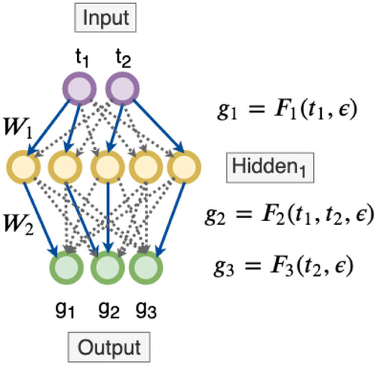We thus want sparse NN weights $W = {W_{1}, W_{2}, \dots, W_{C}}$ to obtain a sparse graph.

FIG. 1.

Using NNs as a multitask learning framework: We start with a fully connected NN indicating all genes are dependent on all the input TFs (dotted black lines). Assume that in the process of discovering the underlying sparse GRN, our algorithm zeroes out all the edge weights except the blue ones. Now, if there is a path from an input TF to an output gene, we then conclude that the output gene is dependent on the corresponding input TF. GRN, gene regulatory network; NN, neural network; TFs, transcription factors.

We can easily obtain the dependency matrix between input TFs and output genes as a matrix multiplication, where $Θ_{p} = Π_{i} | W_{i} | = | W_{1} | \times | W_{2} | \times \dots \times | W_{C} |$ represents the matrix product of the NN weights. This dependency matrix can be directly interpreted as the underlying GRN. Nonzero values in the matrix $Θ_{p}$ correspond to edges between the corresponding pairs of genes.

This multitask NN architecture is superior to boosted decision tree-based formulations as it is more expressive, and does not need the additional post hoc scoring step. It is also more expressive than a simple nonlinear model with additive noise because the NN is jointly optimizing the regression for all the output genes (multitask learning) and this helps it capture the common dependencies between the TFs and output genes. This also makes the NN model more robust toward external noises as jointly optimizing for all the gene expression values will mitigate the effect of any expression value anomalies that seeped in during the experiments.

3.1.1. Designing the unrolled algorithm

Many NN representations can satisfy Equation (1), which leads to multiple possible GRNs. These GRNs will vary mostly in terms of the sparsity obtained and it is hard to tune for the desired sparsity of the GRN manually. Unrolled algorithms help resolve this problem as the sparsity-related hyperparameters (e.g., the weight of the l₁ norm term) can be learned from supervision. Our aim is to get a deep model that optimizes the multitask learning NN along with learning the optimal sparsity pattern using the supervision provided from simulator data. We follow a similar procedure as the unrolled algorithm designed for sparse graph recovery by using the alternative minimization (AM) algorithm (Shrivastava et al., 2020).

3.1.1.1. Identifying the inductive bias

We wish to simultaneously fit the regression formulations in Equation (1) as well as learn the desired sparsity of the underlying GRN. One way to achieve this is to jointly optimize the regression error with an l₁ penalty term over the dependency matrix. Thus, we consider the following nonlinear optimization objective function for the regression with l₁ penalty

where $f_{W} (X_{T}^{k})$ is a NN. Note, $X_{T}^{k}$ represents the expression values for all the $T$ TFs and $X_{g}^{k}$ represents the expression values for all the $g$ genes for the $k^{t h}$ sample or experiment. For example, we can define a two-layer NN with “ReLU” nonlinearity as $f_{W_{1}, W_{2}} (X_{T}^{k}) = W_{2} \cdot R e L U (W_{1} \cdot X_{T}^{k} + b_{1}) + b_{2}$ . We learn the weights ${W_{i}}$ and the biases ${b_{i}}$ while optimizing for Equation (2). The dimensions of the weights and biases are chosen such that the NN input units are equal to “ $T$ ” TFs and the output units are equal to “ $g$ ” genes.

3.1.1.2. Using optimization algorithm as design template

We now identify the iterative updates of a suitable optimization algorithm. Since the mentioned objective is nonlinear, we will need an iterative approach to minimize it w.r.t. $W$ . We apply the AM approach to the optimization given in Equation (2). Our problem becomes easier by using AM as we can get closed form solution of the l₁ penalty term. We introduce an additional Lagrange variable Z, such that $Z = Π_{i} | W_{i} |$ (product of NN weight matrices) and then including the Lagrangian as a square penalty term, we have . Now, alternatively minimize Z and $Θ$ for $l \in [0, L]$ iterations as $W^{(l + 1)} \leftarrow \begin{matrix} a r g m i n \\ w \end{matrix} \sum_{k = 1}^{M} {∥X_{g}^{k} - f_{W} (X_{T}^{k})∥}^{2} + \frac{1}{2} λ {∥Π_{i} | W_{i} | - Z^{l}∥}_{F}^{2} .$ (3)

Z_{l + 1} \leftarrow η_{ρ ∕ λ} (Π_{i} | W_{i}^{(l + 1)} |) .

(4)

The update of Z is of the form $f (Z) + ρ {∥Z∥}_{1}$ , where $f (Z)$ is a convex function. Akin to Shrivastava et al. (2020), the minimizer of this function is the proximal operator given by $η_{ρ ∕ λ} (θ) = s i g n (θ) max (| θ | - ρ ∕ λ, 0)$ .

3.1.1.3. Unrolling the iterations to get deep model

We now unroll the iterative updates to certain iterations, identify key learnable components, and treat the entire unrolled iterations as a single highly recurrent deep model. We identify the proximal operator $η_{ρ ∕ λ}$ and $λ$ as the hyperparameters that control the sparsity of the final graph. We now parameterize them using problem-dependent NNs as $ρ_{n n}, λ_{n n}$ , respectively. These NNs are minimalist in design and take the solution of the previous update to predict the next value, and are learned using supervision. As for Equation (3), we optimize for $W_{i}^{l}$ ( $\forall i$ ) by using standard DL optimizers. The corresponding values of Z^l can be obtained by plugging in the $W_{i}^{l}$ ( $\forall i$ ) in its closed form update, Equation (4). We unroll these updates for L iterations and treat it as a highly structured deep model (Fig. 2).

FIG. 2.

Visualizing the GRNUlar algorithm's architecture. It is a single deep model that is highly structured and recurrent. It takes gene expression data as input and outputs the corresponding GRN. GRNUlar, gene regulatory network unrolled algorithm.

Algorithm 1, GRNUlar-basic, provides a supervised learning framework for the unrolled model directly based on the updates of the AM algorithm, Equations (3) and (4). We typically require $E 1 \sim [200, 400]$ epochs to minimize Equation (3). This slows down the algorithm significantly. To circumvent this issue, we propose a modification to GRNUlar-basic algorithm by using a “good” initialization technique.

We posit that, if we optimize for the first term of Equation (3) beforehand and obtain good initial values of $W^{0}$ , we then just need to do minor adjustments to the $W$ as we update Z and $λ$ . We then just need to unroll the optimization (the new fitDNN-fast function) for only few iterations $P \sim {2, 5, 10}$ . This is a significant reduction in the number of unrolled iterations required over the fitDNN function. The GRNUlar-cell in Algorithm 2 also does not require large number of unrolled iterations L. The NN $ρ_{n n}$ is learning the entry-wise thresholding operation and $λ_{n n}$ learns to update its value from norm difference and its previous value. We observe that in every iteration of Algorithm 2, we optimize the unrolled parameters $ρ_{n n}, λ_{n n}$ (tiny NNs) to learn the underlying graph sparsity from the supervision provided. Thus, we want to highlight that the overall training does not require much training data as well as the number of unrolled iterations.

A note on backpropagation of gradients: While taking the $a r g m i n$ in the fitDNN function given in Algorithm 1, we consider the $λ$ and Z^l as constants. In our PyTorch implementation, we “detach” these variables from the computational graphs while optimizing for $W$ . Ideally we can retain the computational graph while optimizing, but then the memory consumption increases considerably. Another important concern is related to the runtime of Algorithm 1. The fitDNN function is called L times and it initializes a new NN each time and minimizes it for the optimization function to a very low error based on the regularization provided by the $λ$ and Z values.

We typically require $E 1 \sim [200, 400]$ epochs to fit the NN. This slows down the algorithm significantly. To circumvent this issue, we propose a simple modification to GRNUlar-basic algorithm by using a “good” initialization technique as done for the GRNUlar Algorithm 2. We also empirically verify that GRNUlar algorithm performs equivalent to GRNUlar-basic algorithm with significant runtime improvement.

Algorithm 1: GRNUlar-basic
Function covTF $(X, T F s)$ :

Select ${\hat{Σ}}_{T} \subset {\hat{Σ}}_{T}$ an $T \times G$ submatrix using the TFs
return ${\hat{Σ}}_{T}$
Function fitDNN ( $X, Z, λ$ , TFs):
Fit $W$ based on updated regularization terms $λ, Z$
$X_{T}, X_{G} \leftarrow X$ (using the TFs)
$f w^{0} \leftarrow$ initialize neural networks
$W \leftarrow {a r g m i n}_{W} \sum_{k = 1}^{M} {∥X_{G}^{k} - f_{W} (X_{T}^{k})∥}^{2} +$ $\frac{1}{2} λ {∥Π_{i} \| W_{i} \| - Z^{l}∥}_{F}^{2}$
(Using standard DL optimizers for “E1” epochs)
$Θ \leftarrow Π_{i} \| W_{i} \|$
return $Θ$
Function GRNUlar-cell $(X, {\hat{Σ}}_{T}, Θ, Z, λ)$ :
$λ \leftarrow Λ_{n n} ({∥Z - Θ∥}_{F}^{2}, λ)$
$Θ \leftarrow$ fitDNN $(X, Z, λ)$
For all i j do
$ρ_{i j} = ρ_{n n} (Θ_{i j}, {\hat{Σ}}_{T_{i j}}, Z_{i j})$
$Z_{i j} \leftarrow η_{ρ_{i j}} (Θ_{i j})$
return $Θ, Z, λ$
Function GRNUlar $(X)$ :
$λ^{0} \leftarrow 1$
${\hat{Σ}}_{T} \leftarrow$ covTF $(X)$
$Z^{0} = z e r o s (T, G)$
$W_{i' s} \leftarrow$ fitDNN $(X, Z^{0}, λ^{0})$
$Θ^{0} = Π_{i} \| W_{i}^{0} \|$
For $l = 0$ to $L - 1$ do
$Θ^{l + 1}, Z^{l + 1}, λ^{l + 1}$
$\leftarrow$ GRNUlar-cell $(X, {\hat{Σ}}_{T}, Θ^{l}, Z^{l}, λ^{l})$
return $Θ_{L}, Z_{L}$

Algorithm 2: GRNUlar
Function covTF $(X, T F s)$ :

Select ${\hat{Σ}}_{T} \subset \hat{Σ}$ an $T \times G$ submatrix using the TFs
return ${\hat{Σ}}_{T}$
Function fitDNN-fast ( $X, Z, W, λ,$ TFs):
$X_{T}, X_{G} \leftarrow X$ (using the TFs)
For $P = 0$ to $P - 1$ do
$J^{p} = \sum_{k = 1}^{M} ∥ X_{G}^{k} - f w (X_{T}^{k}) ∥^{2} + \frac{λ}{2} ∥ Π_{i} \|W_{i}\| - Z ∥_{F}^{2}$
$w^{p + 1} \leftarrow$ opt-update $(W_{i' s'}^{p} \nabla J^{p})$
$Θ \leftarrow Π_{i} \| W_{i} \|$
return $Θ, w$
Function GRNUlar-cell $(X, {\hat{Σ}}_{T}, w, Θ, Z, λ)$ :
$λ \leftarrow Λ_{n n} ({∥Z - Θ∥}_{F}^{2}, λ)$
$Θ, w \leftarrow$ fitDNN-fast $(X, Z, w, λ)$
For all i, i do
$ρ_{i j} = ρ_{n n} (Θ_{i j}, {\hat{Σ}}_{T_{i j}}, Z_{i j})$
$Z_{i j} \leftarrow η_{ρ_{i j}} (Θ_{i j})$
return $w, Θ, Z, λ$
Function goodINIT $(X, T F s)$ :
$W \leftarrow {a r g m i n}_{W} \sum_{k = 1}^{M} {∥X_{G}^{k} - f_{W} (X_{T}^{k})∥}^{2}$
(Using standard DL optimizers for “E1” epochs)
$Θ \leftarrow Π_{i} \| W_{i} \|$
return $Θ, w$
Function GRNUlar $(X)$ :
$Θ^{0}, w^{0} \leftarrow$ goodINIT $(X)$
$λ^{0} \leftarrow 1$
${\hat{Σ}}_{T} \leftarrow$ covTF $(X)$
$Z^{0} = z e r o s (T, G)$
For $l = 0$ to $L - 1$ do
$w^{l + 1}, Θ^{l + 1}, Z^{l + 1}, λ^{l + 1}$
$\leftarrow$ GRNUlar-cell $(X, {\hat{Σ}}_{T}, w^{l}, Θ^{l}, Z^{l}, λ^{l})$
return $Θ_{L}, Z_{L}$

The GRNUlar model can be thought of as having two stages, namely (refer Fig. 2 and Algorithm 2).

Stage I. We first optimize for the first term in Equation (3) beforehand and obtain “good” initial values of $W^{0}$ . Thereafter, only minor adjustments are needed to $W$ as Z and $λ$ are updated. We then just need to unroll the optimization in the fitDNN-fast function for only few iterations $P \sim {2, 5, 10}$ during Stage II.

Stage II. After getting the “good” initialization from Stage I, the data and parameters are passed through the GRNUlar-cell. It also does not require large number of unrolled iterations L. The NN $ρ_{n n}$ is learning the entry-wise thresholding operation and $λ_{n n}$ learns to update its value from norm difference and its previous value (see Section 3.2). For every iteration of GRNUlar-cell, we optimize the unrolled parameters $ρ_{n n}, λ_{n n}$ (tiny NNs) to learn the underlying graph sparsity from the supervision provided. We highlight here that the overall training does not require much data as well as the number of unrolled iterations.

3.2. A note on parameterizing the NNs of unrolled algorithms

The general idea of NN-based parameterization: For the GRNUlar algorithm, we can further parameterize the optimizer update given in “fitDNN-fast” function of Algorithm 2 and learn it from the supervision provided, similar to $Λ_{n n}$ . In our current implementation, we use the “adam” optimizer. We want to highlight that our technique of parameterization in an unrolled manner is very generic and can be used for any off-the-shelf optimizer.

For instance, consider the example of parameterizing gradient descent optimizer that is realized using the $Λ_{n n}$ update. We just need to define the NN-based parameterization in a way that is more generic than the optimizer's update equation. The NN-based update $λ^{t + 1} \leftarrow Λ_{n n} ({∥Z - Θ∥}_{F}^{2}, λ^{t})$ subsumes the standard gradient descent update given by $λ^{t + 1} \leftarrow λ^{t} - α {∥Z - Θ∥}_{F}^{2}$ .

4. TRAINING THE GRNUlar FRAMEWORK

GRNs are typically sparse and so we want our loss function to be robust enough to recover sparse edges. There are many techniques developed to train in a cost-sensitive setting where in the data we have very few positive data points (edges present) versus large number of negative data points (edges absent) (Chawla et al., 2002; Thai-Nghe et al., 2010; Shrivastava et al., 2015; Bhattacharya et al., 2017). Since there are multiple metrics such as precision, recall, and F1 score that are commonly used for evaluation of the recovered GRNs, it will be useful to define a loss function that can find a desirable balance between them.

To address the mentioned concerns, we develop a differentiable version of the $F_{β}$ score. Let $Θ^{p}$ represent our predicted graph (adjacency matrix) and let $Θ^{*}$ be the true underlying graph. We assume that all the entries of $Θ \in [0, 1]$ . We can write the true positives (TPs), true negatives (TNs), false positives (FPs), and false negatives (FNs) as follows: $\begin{matrix} T P = < Θ^{p}, Θ^{*} >; F P = < Θ^{p}, 1 - Θ^{*} >; \\ F N = < 1 - Θ^{p}, Θ^{*} >; T N = < 1 - Θ^{p}, 1 - Θ^{*} >; \end{matrix}$ (5)

where $< \cdot, \cdot >$ represents matrix inner product, which is the summation of entry-wise products. Based on the mentioned differentiable representations, we define differentiable $F_{β}$ score and the corresponding loss function as $\begin{matrix} F_{β} = (1 + β^{2}) \cdot T P ∕ ((1 + β^{2}) \cdot T P + β^{2} \cdot F N + F P); L_{F_{β}} = 1 - F_{β} \end{matrix} .$ (6)

A value of $β > 1$ weighs recall higher than precision as it emphasizes the FNs. Similarly, having $β < 1$ attenuates the influence of FNs and thus weigh recall lower than precision.

We define a loss function between the predicted and true adjacency matrix as the combination of the mean square error (MSE) (or Frobenius norm) loss and the $L_{F_{β}}$ loss. It is often tricky to jointly optimize and balance between multiple loss functions. Following the loss balancing technique described in Rajbhandari et al. (2019), we introduce a balancing ratio $r = L_{F_{β}} ∕ L_{m s e}$ that adjusts the scales of both the losses. Note that “r” is detached from computational graph to facilitate backpropagation of gradients. $L o s s = r . {∥Π_{i} | W_{i}^{(L)} | - W^{*}∥}_{F}^{2} + L_{F_{β}} (tanh {Π_{i} | W_{i}^{(L)} |}, W^{*}) .$ (7)

The matrix $W^{*} \in {0, 1}^{(g \times T)}$ represents the ground truth network, where 1 indicates presence of an edge between $(t, g)$ . To ensure that the entries of $Θ^{p} \in [0, 1]$ , we pass it through the $tanh {| Θ^{p} |}$ operation. We optimize the loss function over the average of data pairs from simulator so that the learned architecture is able to perform well over a family of problem instances.

5. EXPERIMENTAL RESULTS

5.1. Methods compared and evaluation measures

We use the area under the receiver operating characteristics (AUROC) and the area under the precision recall curve (AUPRC) values for evaluation (Chen and Mar, 2018; Dibaeinia and Sinha, 2019) and comparison of various methods. We compared GRNUlar with GRNBoost2 (Moerman et al., 2019, GENIE3 (Vân Anh Huynh-Thu et al., 2010), and GLAD (Shrivastava et al., 2020).

GRNBoost2 and GENIE3 are representative of regression-based methods, and are among the top performers for single-cell expression data (Pratapa et al., 2020). We used the Arboreto package to run these algorithms (Moerman et al., 2019). We did extensive fine tuning of the hyperparameters for both the methods using the training/valid data and reported results on the test data. “Method+TF” indicates that TF information was utilized for GRN recovery.

GLAD by Shrivastava et al. (2020) is an unrolled algorithm designed for sparse graph recovery. It is based on unrolling the iterations of an alternate minimization algorithm for the graphical lasso problem. It fits a multivariate Gaussian distribution on the input gene expression data with an l₁ normalization term. We modified the GLAD algorithm to take into account TF information, called GLAD+TF, by using a post hoc masking operation that only retains the edges having at least one node as a TF. We used the standard initialization as recommended by the authors.

We chose the number of unrolled iterations L = {15, 30}. For the GRNUlar model, we used the same initialization of the thresholding parameters $ρ_{n n}, λ_{n n}$ as proposed for the GLAD model. Now, we need to decide the dimensions of NN that fits the regression in the fitDNN-fast function. Our general strategy is to have number of hidden layers, $d e p t h \geq 2$ , of the NN. We roughly choose the number of hidden units in layer “j” as $H_{j} \geq 4 \cdot H_{j - 1}$ and we also satisfy $T F s \leq H_{1}$ . We empirically observed that we need around [200, 500] iterations to fit the NN in the goodINIT function. We chose the unroll parameters L = 15 and the values of P = {5, 10, 20} with NN having two or three layers.

For both the unrolled methods, we chose two models based on AUPRC and AUROC results on the validation data. We use the scaled loss function [Eq. (7)] to jointly optimize for MSE and $F_{β}$ loss. The values of $β$ used in our experiments were chosen from the set {0.5, 1, 2, 5}. We implemented the unrolled algorithms using PyTorch and ran on Nvidia P100 GPUs. We observed that for these unrolled algorithm-based approaches, GRNUlar in general outperforms GLAD+TF. This is probably due to the difference in the choice of inductive bias for designing their architectures as former is based on the regression-based formulation, whereas the architecture of the latter is based on the graphical lasso-based formulation.

5.2. Details of SERGIO simulator for clean and noisy settings

SERGIO provides a list of parameters to simulate cells from different types of biological processes and gene-expression levels with various amounts of intrinsic and technical noise. We simulated cells from multiple steady states. When simulating data with no technical noise (what we refer to as clean data), we set the following parameters: sampling-state = 15 (determines the number of steps of simulations for each steady state); noise-param $\sim U [0.1, 0.3]$ (controls the amount of intrinsic noise); noise-type = “dpd” (the type of intrinsic noise is dual production decay noise, which is the most complex out of all types provided); we set genes' decay parameter to 1.

The parameters required to decide the master regulators' basal production cell rate for all cell types—low expression range of production cell rate $\sim U [0.2, 0.5]$ and high expression range of cell rate $\sim U [0.7, 1]$ . We chose $K \sim U [1, 5]$ , where “K” denotes the maximum interaction strength between master regulators and target genes. Positive strength values indicate activating interactions and negative strength values indicate repressive interactions and ±1 signs are randomly assigned. We added the dropout events that are considered to be a major source of technical noise in real data. Parameters that control the amount of dropouts include shape (which was set to 20) and percentile, which we varied among the values $q = {25, 50, 75}$ . Larger q corresponds to higher technical noise. All other parameters were set to default values.

5.3. Evaluating GRN inference methods on synthetic data

We conducted an exploratory study to gauge the generalization ability of GRNUlar for the GRN inference task. To provide supervision, we used the SERGIO simulator. To create random directed graphs (GRNs), we first decided on the number of TFs or master regulators. Then, we randomly added edges between the TFs and the other genes based on sparsity requirements. Also, we randomly added some edges between the TFs themselves but excluded any self-regulation edges and maintained connectivity of the graph.

The graph is then provided as input to the SERGIO simulator to generate corresponding gene expression data. For the experiments in this subsection, we took train/valid/test = $20 ∕ 20 ∕ 50$ graphs, respectively, with the number of genes D = 100. All these graphs were sampled from similar settings. We usually choose the ratio of TFs to the total number of genes as 0.1 (∼10 TFs for D = 100) and sparsity of training graphs to be 0.1. We wish to highlight that many graphs are not needed to train the unrolled models as we are primarily learning the sparsity pattern from supervision and need small NNs for the same (refer fig. 3 in Shrivastava et al., 2020).

FIG. 3.

Clean data setting of the SERGIO simulator with D = 100 genes. As the number of cell types increases from C = 2 to C = 10, we see that the AUPRC values increase in general. The unrolled algorithms in general outperform the traditional methods. AUPRC, area under the precision recall curve.

From the literature on sample complexity theory of sparse graph recovery (e.g., see, Ravikumar et al., 2011), we know that recovery of the underlying graph improves with increasing number of samples. Hence, we ran our experiments with varying number of the total single cells, M = {100, 500, 1K, 5K, 10K}.

We also observed that varying the number of cell types (corresponding to the number of clusters of the cells) of the SERGIO simulator considerably affects GRN inference results, so we also evaluated the methods by varying the number of cell types of the simulator C = {2, 5, 10}. We adjusted the number of cells per cell type to maintain the same total number of cells. Section 5.2 contains detailed description of SERGIO settings. For experiments in this subsection, each data point in the plots represents its value along with standard deviation over the test graphs.

5.3.1. Clean: simulated data with no technical noise

The “clean” gene expression data from SERGIO follow all the underlying kinetic equations but exclude all the external technical noises. These data can be considered as being recorded with no technical errors. Figure 3 compares different methods on their AUPRC performance on varying number of cells and number of cell types. For GRNUlar model we chose two-layer NN with p = 5, H_d = {40, 60, 100}, L = 15, and vary $β = {2, 5}$ in the loss function. The best model was chosen based on the validation results. We observe that GRNUlar consistently outperforms other methods.

5.3.2. Noisy: simulated data with technical noise

We evaluate on the more challenging and realistic noisy settings. We limit varying the technical noise to dropouts while keeping the default settings for other SERGIO parameters. For higher levels of dropouts, researchers sometimes resort to data imputation techniques (which attempt to recover the number of molecules being dropped) as a preprocessing step that marginally improves results. For these experiments, we report results without the imputation preprocessing step and compare all methods directly on the noisy data obtained from the simulator.

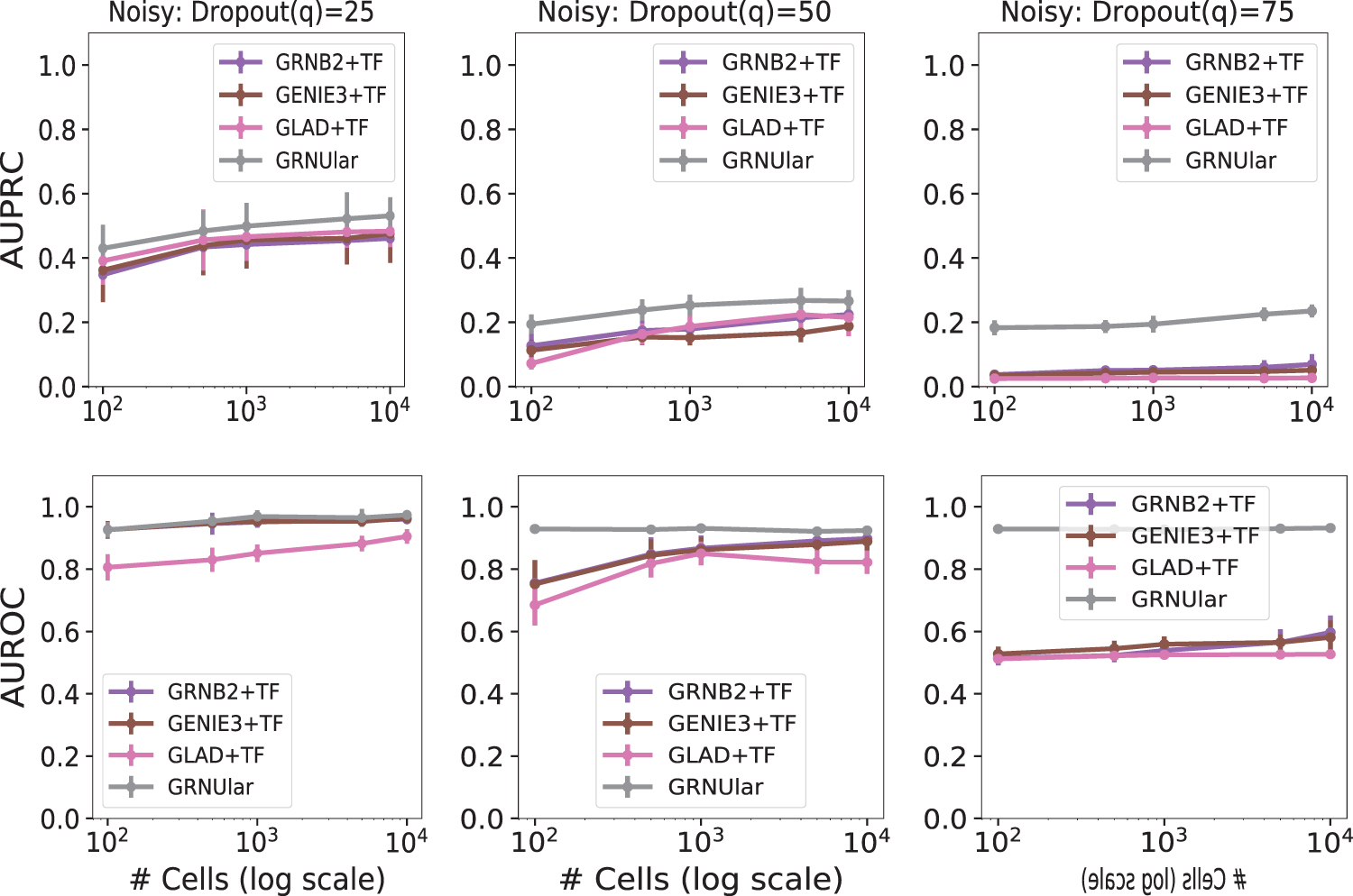
While training the models, we train on data with low dropout rates $q = {0, 25}$ and use the same models to predict networks on data with higher dropout rates. In Figure 4, as we move toward the right, dropout percentile increases and we can observe deterioration in AUPRC values, although the GRNUlar model's AUROC performance is quite robust with increasing dropouts. Even in the case of 75% dropout value, where the other algorithms almost give output equivalent to random prediction, GRNUlar is able to handle this high percentage of missing information.

FIG. 4.

Noisy data setting of the SERGIO simulator with dropout shape = 20, D = 100, and C = 5. We vary the dropout percentile values as [25, 50, 75] in both the upper panels (AUPRC values) and the lower panel (AUROC values). Larger q corresponds to higher technical noise. GRNUlar has a clear advantage in noisy settings. AUROC, area under the receiver operating characteristics.

5.4. Realistic data from SERGIO: Escherichia coli and yeast

The challenge for data-driven models is to be able to generalize to real data sets. Thus, it is important to test the ability of the unrolled algorithms to generalize over different settings from that of the training. To perform this study, we make use of the realistic data sets provided by the SERGIO simulator. They provide three scRNA-Seq data sets DS1, DS2, and DS3 that are generated from input GRNs with 100, 400, and 1200 genes, respectively. These networks were sampled from real regulatory networks of Escherichia coli and Saccharomyces cerevisiae.

For each data set, the settings are number of cell types C = 9, total number of single cells M = 2700, and there are 300 cells per cell type. Each data set was synthesized in 15 replicates by re-executing SERGIO with identical parameters multiple times. The parameters were configured such that the statistical properties of these synthetic data set are comparable with the mouse brain, given in Zeisel et al. (2015).

We defined our training and testing settings such that there were considerable differences between them. We used all of the DS1, DS2, and DS3 data sets for testing. We train on data with settings similar to DS1, specifically the parameters such as production cell rates, decays, noise parameter, and interaction strength. We trained with no dropouts as opposed to 82% dropout percentile in the case of the DS data sets. The data sets DS2 and DS3 are completely different from training data (and DS1) in terms of the underlying GRN, as well as the corresponding SERGIO parameters are sampled from different range of values. For details, refer to table 1 and appendix tables S1, S3 in Dibaeinia and Sinha (2019) for more insight into the differences in SERGIO parameter settings.

Table 1.

Details of Expression Data from the BEELINE Framework

Data	No. of TFs	No. of Expts
mDC	42	383
mESCs	100	421
mHSCs-E	69	1071
mHSCs-GM	74	889
mHSCs-L	83	847
hESCs	86	758
hHep	56	425

Total number of genes for each data is 500 (highest varying genes).

Experiments: hESCs, human embryonic stem cells; hHep, human mature hepatocytes; mDCs, mouse dendritic cells; mESCs, mouse embryonic stem cells; mHSCs-E, mouse hematopoietic stem cells-erythroid; mHSCs-GM, mouse hematopoietic stem cells-granulocyte-macrophage; mHSCs-L, mouse hematopoietic stem cells-lymphoid; TFs, transcription factors.

5.4.1. GRNUlar settings

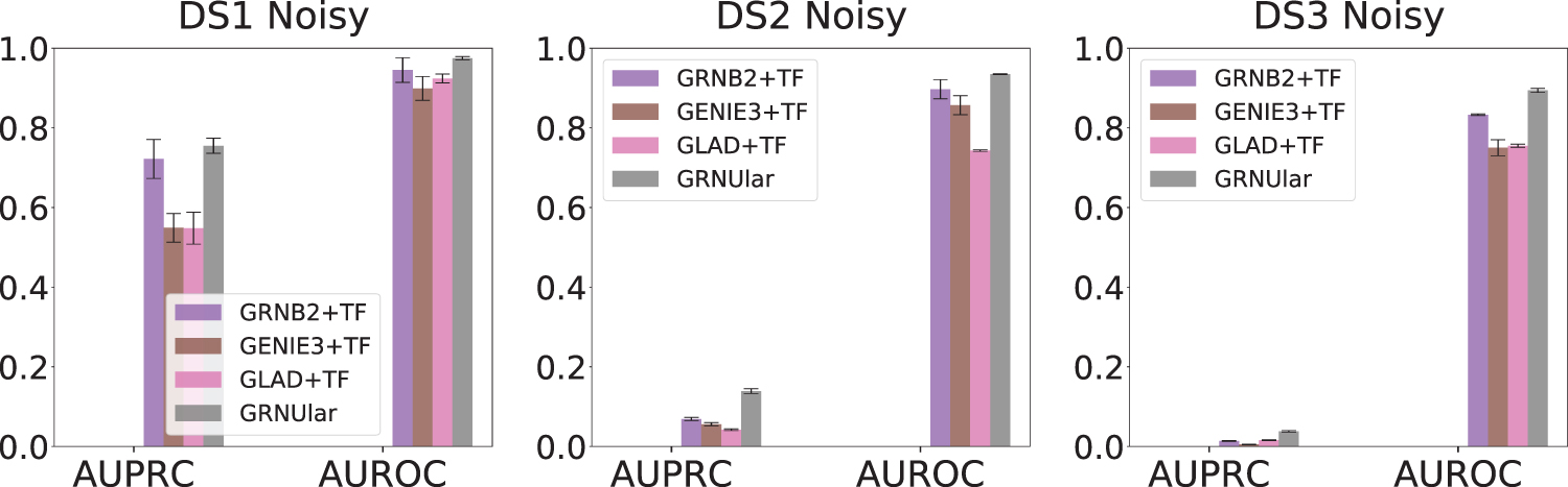
We used a two-layer NN in the fitDNN-fast function for these experiments with a single hidden layer H₁. Following our strategy to choose the dimensions, $H_{1} \sim 4 \times T F s$ . The number of TFs in DS1/DS2/DS3 is 10/37/127, respectively. So, we chose $H_{1} = 40 ∕ 200 ∕ 500$ , respectively, as the hidden layer dimensions. The other parameter settings remain similar to those mentioned in the previous subsections. Figure 5 shows that GRNUlar performs better on these realistic data sets.

FIG. 5.

Realistic data from SERGIO of Escherichia coli and yeast—(noisy settings, dropout percentile = 82%). We report the average results over 15 test graphs in the noisy settings. GRNUlar gives notable AUPRC values and it outperforms other methods.

5.5. Real scRNA-Seq data sets

We evaluated 21 gene expression data sets from the human and mouse species and their corresponding ground truth networks (Pratapa et al., 2020).

We evaluated different methods on seven data sets from five experiments that include human mature hepatocytes (Camp et al., 2017), human embryonic stem cells (hESCs) (Chu et al., 2016), mouse embryonic stem cells (mESCs) (Hayashi et al., 2018), mouse dendritic cells (Shalek et al., 2014), and three lineages of mouse hematopoietic stem cells (Nestorowa et al., 2016): erythroid lineage, granulocyte–macrophage lineage, and lymphoid lineage.

These are the same data sets used in Pratapa et al. (2020) and we use their corresponding ground truth networks for our experiments as well. For each data set, there are three versions of ground truth networks: cell-type-specific ChIP-Seq, nonspecific ChIP-Seq, and functional interaction networks collected from STRING. We then have in all 21 different data pairs, 7 different types of expression data evaluated against 3 different types of ground truth.

5.5.1. Preprocessing the real data

For each gene expression data and its corresponding network, we first sorted all the genes according to their variance and select the top 500 varying genes. From the list of known TFs, we only considered all the TFs whose variance had p-value at most 0.01. We then found the intersection between the top 500 varying genes and all the TFs to get a subset of genes that act as the TFs (Table 1). Then, we selected the subgraph of top 500 varying genes from the underlying GRN as our ground truth for evaluation.

5.5.2. Training details

We train on the expression data that is similar to the SERGIO settings for the DS2 data set as it has similar number of genes as the real data. We chose the underlying GRNs for supervision as the random graphs described in Section 5.3. We fixed the number of genes D = 400, the number of cell types C = 9, and total number of single cells M = 2700. The GRNUlar settings were $P = {2, 5, 10}, L = 15, H_{d} = {200}$ with two-layer NN.

In general for real data, we observed very low AUPRC values (refer Fig. 6); this is primarily due to the highly skewed ratio between true edges and total possible edges (Davis and Goadrich, 2006; Chen and Mar, 2018). The GRNUlar algorithm clearly outperformed other methods in all test settings. We can further improve the results by tuning the SERGIO simulator settings closer to the real data under consideration. Section 6.1 compares the inference runtimes for various methods.

FIG. 6.

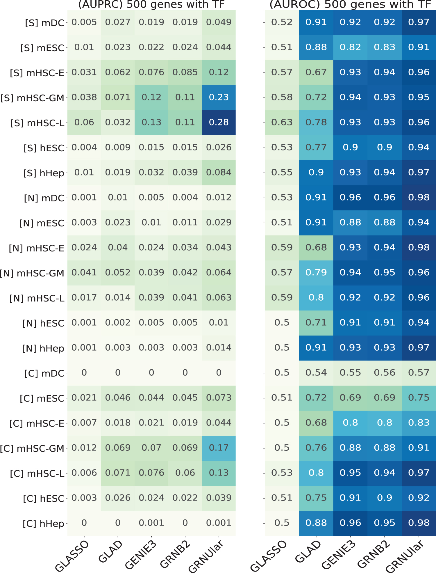
Heatmap of AUPRC and AUROC values of the real data from the BEELINE framework by Pratapa et al. (2020). We ran all the methods including the TF information. [S]/[N]/[C] represent the ground truth networks [String-network]/[nonspecific-ChIP-seq-network]/[cell-type-specific-ChIP-seq] respectively. Data of the species [m] mouse and [h] human were used. GRNUlar performs better than the other algorithms in both the metrics. hESCs, human embryonic stem cells; hHep, human mature hepatocytes; mDCs, mouse dendritic cells; mESCs, mouse embryonic stem cells; mHSCs-E, mouse hematopoietic stem cells-erythroid; mHSCs-GM, mouse hematopoietic stem cells-granulocyte-macrophage; mHSCs-L, mouse hematopoietic stem cells-lymphoid.

6. ANALYZING THE mESC NETWORK PREDICTED BY GRNUlar

We analyzed the network predicted by GRNUlar from the mESC data set (Hayashi et al., 2018). We chose TFs and genes corresponding to gene ontology terms related to ESC differentiation and cell fate toward endodermal cells as in this data set the ESCs are induced to differentiate into primitive endoderm cells (Hayashi et al., 2018). From BioMart (Kinsella et al., 2011) we obtained 286 genes. We took the intersection between these genes with our predicted GRN (with 500 genes) and found 32 genes.

We first compared the interaction scores predicted by GRNUlar among all 500 genes and the scores among the 32 genes, without applying any threshold. We found that the latter set of scores is significantly higher than the former set of scores (Fig. 7). This means there are more regulatory activities among the genes related to the expected biological processes compared with all the genes selected by variation. We then set the threshold for interaction score as 0.22, and obtained the network shown in Figure 9. In this network, the TFs SOX7, SOX17, MTF2, GATA6, and CITED2 are known TFs in either stem cell differentiation or embryo development; NOTCH1 and RBPJ are TFs in the NOTCH pathway that controls cell fate specification (www.genecards.org). The TFs with highest interaction scores are highly relevant TFs for the cells under study.

FIG. 7.

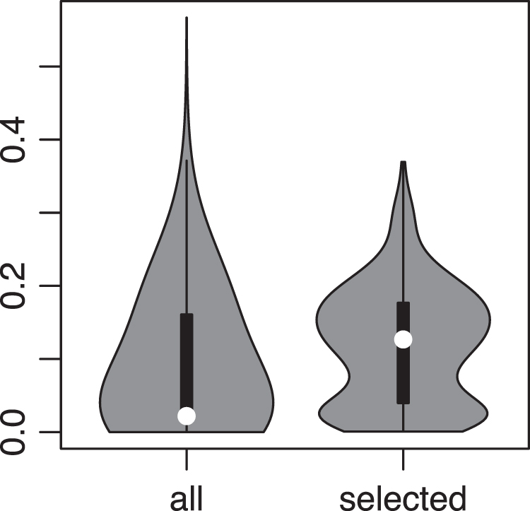
Violin plot comparing the scores of all interactions in the 500 genes (left) and interaction scores between the 32 genes (right). Wilcoxon p-value is 1.3e⁻¹⁴.

We now show how our predicted interactions may bring new biological insights. For instance, we noticed that one of the target genes of SOX7 with strong interaction is CFC1. From ChIP-Seq experiments (the [cell-type-specific-ChIP-Seq] ground truth network mentioned previously), SOX2 is a TF for CFC1.

However, we predicted SOX7 and SOX17 as the TFs for CFC1 in our results. We note that the data set consists of ESCs differentiating into primitive endoderm cells, and SOX2 is a key TF in mESCs governing the pluripotency of the cells (Masui et al., 2007). As the cells differentiate, the pluripotency goes down, so the SOX2 function may also decrease. To verify this, we use the pseudotime of the cells obtained from Pratapa et al. (2020), which was inferred with Slingshot (Street et al., 2018), and visualize the gene expression levels of CFC1, SOX2, SOX7, and SOX17 (Fig. 8). For readability, we plot the actual gene expression levels cell by cell only for CFC1, and for the SOX TFs we plot the fitted lines of their expression levels obtained using LOESS regression. The dashed lines represent the standard deviation.

FIG. 8.

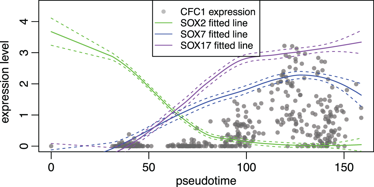
Comparison of gene expression patterns over the pseudotime for CFC1 and the SOX family TFs.

FIG. 9.

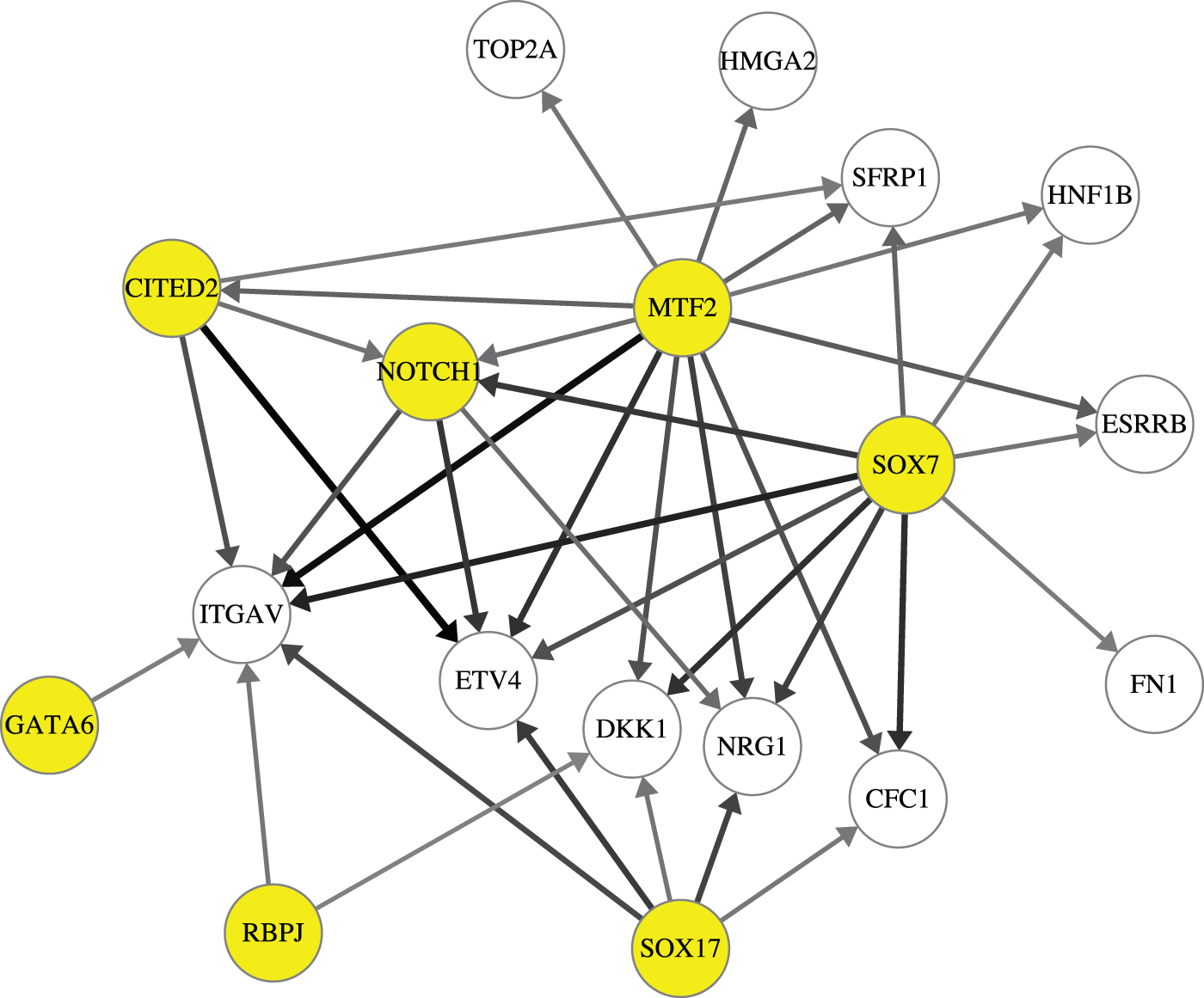
A subnetwork [completed partially directed acrylic graph (CPDAG)] with genes related to stem cell differentiation from GRNUlar predicted network. TFs are the nodes with yellow background. Darker edges mean higher predicted score for the interaction.

We see that indeed the SOX2 expression decreases along the pseudotime, and the expression levels of CFC1, SOX7, and SOX17 increase. The fitted lines of SOX7 and SOX17 show that they are much better predictors for the expression of CFC1 than SOX2. Indeed, it is discussed that SOX7 and SOX17 are highly related members of the SOX family and their high expression in ESCs are correlated with a downregulation of the pluripotency and an upregulation of the primitive endoderm-associated program (Sarkar and Hochedlinger, 2013).

This example showcases how we can use predicted regulatory networks to find regulatory pathways for a specific biological program. Some of these may already have evidence in the literature but some may be new and our prediction can be used to provide hypothesis for further experimental validation.

6.1. Runtimes of different methods

Tables 2 and 3 show the inference time required for different methods with the TF information included. We run different methods on different platforms and hence comparing them directly is not fair. Although we include them to give an idea of the runtimes to the reader.

Table 2.

Inference Runtimes for the GRNUlar Model with Two-Layer Neural Network, As We Vary the Hidden Layer Dimensions H_d

Time (seconds)	H_d = 200	H_d = 500	H_d = 1000
GRNUlar [gpu]	0.89	1.33	2.10

The time is reported for one complete forward call (goodINIT and fitDNN-fast) for D = 1200 genes graph. Other relevant parameters settings were p = 5, L = 15, DNN epochs E1 = 400.

GRNUlar, Gene Regulatory Network Unrolled algorithm.

Table 3.

Inference Times for Different Methods on D = 1200 Genes Graph

Methods	GLASSO [cpu]	GRNB2 [cpu]	GENIE3 [cpu]	GLAD [gpu]	GRNUlar [gpu]
Time (secs)	180	612	1020	0.79	1.33

The unrolled algorithms were run on GPUs (NVIDIA P100s), whereas the traditional methods were run on CPU having a single node with 28 cores.

GENIE3; GLAD; GLASSO; GRNB2.

7. CONCLUSIONS AND DISCUSSIONS

We present a deep unrolled supervised learning framework GRNUlar for GRN inference from scRNA-Seq data. The GRNUlar model combines the expressive ability of NNs to capture complex regulation dependencies that manifest in expression data with unrolled learning of sparse graphical models to effectively emulate sparsity of the regulatory networks observed in the real world. We demonstrate that GRNUlar consistently outperforms the representative best-in-class methods on both simulated and real data sets, especially in the more realistic case of added technical noise. Our DL framework accommodates nonlinearity of the regulatory relationships between TFs and genes, and demonstrates high tolerance to technical noise in data.

The unrolled algorithm we proposed is the first supervised DL method for GRN inference from scRNA-Seq data. Our model learns the characteristics of the underlying network through simulated data from GRN-guided simulators such as SERGIO, and demonstrates the novel and effective use of these simulators in training DL models, apart from their traditional use in benchmarking computational methods. Similar techniques can be investigated for other analysis tasks on single-cell data such as clustering and trajectory inference (Luecken and Theis, 2019), by using available realistic simulators for scRNA-Seq data (Dibaeinia and Sinha, 2019; Zhang et al., 2019).

Footnotes

ACKNOWLEDGMENTS

We thank Aditya Pratapa and T.M. Murali for sharing the gold standard networks for real data used in their article (Pratapa et al., ).

AUTHOR DISCLOSURE STATEMENT

The authors declare they have no conflicting financial interests.

FUNDING INFORMATION

This study is supported, in part, by the National Science Foundation under IIS-1841351 and OAC-1828187.

References

Aibar

, González-Blas

C.B.

, Moerman

, et al. 2017. Scenic: Single-cell regulatory network inference and clustering. Nat. Methods. 14, 1083–1086.

Belilovsky

, Kastner

, Varoquaux

, et al. 2017. Learning to discover sparse graphical models, 440–448. Proceedings of the 34th International Conference on Machine Learning, Volume 70.

Bhattacharya

, Rajan

, and Shrivastava

2017. ICU mortality prediction: A classification algorithm for imbalanced datasets. Proceedings of the AAAI Conference on Artificial Intelligence, Volume 31.

Camp

J.G.

, Sekine

, Gerber

, et al. 2017. Multilineage communication regulates human liver bud development from pluripotency. Nature. 546, 533–538.

Chan

T.E.

, Stumpf

M.P.

, and Babtie

A.C.

2017. Gene regulatory network inference from single-cell data using multivariate information measures. Cell Systems. 5, 251–267.

Chawla

N.V.

, Bowyer

K.W.

, Hall

L.O.

, et al. 2002. Smote: Synthetic minority over-sampling technique. J. Artif. Intell. Res. 16, 321–357.

Chen

, Guo

, Mishra

S.K.

, et al. 2015. Single-cell transcriptional analysis to uncover regulatory circuits driving cell fate decisions in early mouse development. Bioinformatics. 31, 1060–1066.

Chen

, and Mar

J.C.

2018. Evaluating methods of inferring gene regulatory networks highlights their lack of performance for single cell gene expression data. BMC Bioinformatics. 19, 232.

Chen

, Li

, Umarov

, et al. 2020. RNA secondary structure prediction by learning unrolled algorithms. arXiv preprint arXiv:2002.05810.

10.

Chickering

D.M.

2002. Learning equivalence classes of Bayesian-network structures. J. Mach. Learn. Res. 2, 445–498.

11.

Chu

L.-F.

, Leng

, Zhang

, et al. 2016. Single-cell RNA-Seq reveals novel regulators of human embryonic stem cell differentiation to definitive endoderm. Genome Biol. 17, 173.

12.

Davis

, and Goadrich

2006. The relationship between precision-recall and ROC curves, 233–240. Proceedings of the 23rd International Conference on Machine Learning.

13.

Dibaeinia

, and Sinha

2019. A single-cell expression simulator guided by gene regulatory networks. bioRxiv. 716811.

14.

Friedman

, Hastie

, and Tibshirani

2008. Sparse inverse covariance estimation with the graphical lasso. Biostatistics. 9, 432–441.

15.

Goodfellow

, Bengio

, Courville

, et al. 2016. Deep Learning, Volume 1. MIT Press, Cambridge, MA.

16.

Hamey

F.K.

, Nestorowa

, Kinston

S.J.

, et al. 2017. Reconstructing blood stem cell regulatory network models from single-cell molecular profiles. Proc. Natl. Acad. Sci. USA. 114, 5822–5829.

17.

Haury

A.-C.

, Mordelet

, Vera-Licona

, et al. 2012. Tigress: Trustful inference of gene regulation using stability selection. BMC Syst. Biol. 6, 145.

18.

Hayashi

, Ozaki

, Sasagawa

, et al. 2018. Single-cell full-length total RNA sequencing uncovers dynamics of recursive splicing and enhancer RNAs. Nat. Commun. 9, 619.

19.

Huynh-Thu

V.A.

and Sanguinetti

2015. Combining tree-based and dynamical systems for the inference of gene regulatory networks. Bioinformatics. 31, 1614–1622.

20.

Irrthum

, Wehenkel

, Geurts

, et al. 2010. Inferring regulatory networks from expression data using tree-based methods. PLoS One. 5, e12776.

21.

Kim

2015. PPCOR: An R package for a fast calculation to semi-partial correlation coefficients. Commun. Stat. Appl. Methods. 22, 665.

22.

Kinsella

R.J.

, Kähäri

, Haider

, et al. 2011. Ensembl biomarts: A hub for data retrieval across taxonomic space. Database. 2011.

23.

Kiselev

V.Y.

, Andrews

T.S.

, and Hemberg

2019. Challenges in unsupervised clustering of single-cell RNA-Seq data. Nat. Rev. Genet. 20, 273–282.

24.

Lim

C.Y.

, Wang

, Woodhouse

, et al. 2016. Btr: Training asynchronous boolean models using single-cell expression data. BMC Bioinformatics. 17, 355.

25.

Luecken

M.D.

and Theis

F.J.

2019. Current best practices in single-cell RNA-Seq analysis: A tutorial. Mol. Syst. Biol. 15, e8746.

26.

Masui

, Nakatake

, Toyooka

, et al. 2007. Pluripotency governed by SOX2 via regulation of OCT3/4 expression in mouse embryonic stem cells. Nat. Cell Biol. 9, 625–635.

27.

Matsumoto

, Kiryu

, Furusawa

, et al. 2017. SCODE: An efficient regulatory network inference algorithm from single-cell RNA-Seq during differentiation. Bioinformatics. 33, 2314–2321.

28.

Moerman

, Aibar Santos

, Bravo González-Blas

, et al. 2019. GRNBOOST2 and ARBORETO: Efficient and scalable inference of gene regulatory networks. Bioinformatics. 35, 2159–2161.

29.

Nestorowa

, Hamey

F.K.

, Pijuan Sala

, et al. 2016. A single-cell resolution map of mouse hematopoietic stem and progenitor cell differentiation. Blood J. Am. Soc. Hematol. 128, e20–e31.

30.

Papili Gao

, Ud-Dean

S.M.

, Gandrillon

, et al. 2018. Sincerities: Inferring gene regulatory networks from time-stamped single cell transcriptional expression profiles. Bioinformatics, 34, 258–266.

31.

Pratapa

, Jalihal

A.P.

, Law

J.N.

, et al. 2020. Benchmarking algorithms for gene regulatory network inference from single-cell transcriptomic data. Nat. Methods. 17, 147–154.

32.

Rajbhandari

, Shrivastava

, and He

2019. ANTMAN: Sparse low-rank compression to accelerate RNN inference. arXiv preprint arXiv:1910.01740.

33.

Ravikumar

, Wainwright

M.J.

, Raskutti

, et al. 2011. High-dimensional covariance estimation by minimizing l1-penalized log-determinant divergence. Electr. J. Stat. 5, 935–980.

34.

Razaghi-Moghadam

and Nikoloski

2020. Supervised learning of gene-regulatory networks based on graph distance profiles of transcriptomics data. NPJ Syst. Biol. Appl. 6, 1–8.

35.

Ruder

2017. An overview of multi-task learning in deep neural networks. arXiv preprint arXiv:1706.05098.

36.

Sanchez-Castillo

, Blanco

, Tienda-Luna

I.M.

, et al. 2018. A Bayesian framework for the inference of gene regulatory networks from time and pseudo-time series data. Bioinformatics. 34, 964–970.

37.

Sarkar

, and Hochedlinger

2013. The SOX family of transcription factors: Versatile regulators of stem and progenitor cell fate. Cell Stem Cell. 12, 15–30.

38.

Shalek

A.K.

, Satija

, Shuga

, et al. 2014. Single-cell RNA-Seq reveals dynamic paracrine control of cellular variation. Nature. 510, 363–369.

39.

Shrivastava

, Huddar

, Bhattacharya

, et al. 2015. Classification with imbalance: A similarity-based method for predicting respiratory failure, 707–714. 2015 IEEE International Conference on Bioinformatics and Biomedicine (BIBM), IEEE.

40.

Shrivastava

, Chen

, et al. 2020. {GLAD}: Learning sparse graph recovery. International Conference on Learning Representations. Available at: https://openreview.net/forum?id=BkxpMTEtPB. Last viewed on December, 30, 2021.

41.

Specht

A.T.

, and Li

2017. Leap: Constructing gene co-expression networks for single-cell RNA-Sequencing data using pseudotime ordering. Bioinformatics. 33, 764–766.

42.

Street

, Risso

, Fletcher

R.B.

, et al. 2018. Slingshot: Cell lineage and pseudotime inference for single-cell transcriptomics. BMC Genomics,, 19, 477.

43.

Thai-Nghe

, Gantner

, and Schmidt-Thieme

2010. Cost-sensitive learning methods for imbalanced data, 1–8. The 2010 International Joint Conference on Neural Networks (IJCNN), IEEE.

44.

Vallejos

C.A.

, Risso

, Scialdone

, et al. 2017. Normalizing single-cell RNA sequencing data: Challenges and opportunities. Nat. Methods. 14, 565–571.

45.

Vân Anh Huynh-Thu

A.I.

, Wehenkel

, and Geurts

2010. Inferring regulatory networks from expression data using tree-based methods. PLoS One. 5.

46.

Woodhouse

, Piterman

, Wintersteiger

C.M.

, et al. 2018. SCNS: A graphical tool for reconstructing executable regulatory networks from single-cell genomic data. BMC Syst. Biol. 12, 1–7.

47.

Yuan

, and Bar-Joseph

2019. Deep learning for inferring gene relationships from single-cell expression data. Proc. Natl. Acad. Sci. USA. 116, 27151–27158.

48.

Zeisel

, Muñoz-Manchado

A.B.

, Codeluppi

, et al. 2015. Brain structure. cell types in the mouse cortex and hippocampus revealed by single-cell RNA-Seq. Science. 347, 1138–1142.

49.

Zhang

, Xu

, and Yosef

2019. Simulating multiple faceted variability in single cell RNA sequencing. Nat. Commun. 10, 2611.