Genome-Wide Association with Uncertainty in the Genetic Similarity Matrix

Abstract

Genome-wide association studies (GWASs) are often confounded by population stratification and structure. Linear mixed models (LMMs) are a powerful class of methods for uncovering genetic effects, while controlling for such confounding. LMMs include random effects for a genetic similarity matrix, and they assume that a true genetic similarity matrix is known. However, uncertainty about the phylogenetic structure of a study population may degrade the quality of LMM results. This may happen in bacterial studies in which the number of samples or loci is small, or in studies with low-quality genotyping. In this study, we develop methods for linear mixed models in which the genetic similarity matrix is unknown and is derived from Markov chain Monte Carlo estimates of the phylogeny. We apply our model to a GWAS of multidrug resistance in tuberculosis, and illustrate our methods on simulated data.

1. INTRODUCTION

Genome-wide association studies (GWASs) are designed to identify the genetic variants affecting phenotypes of interest such as multidrug resistance in tuberculosis (MDR-TB) (Price et al, 2006; Zhang et al, 2010). Classic approaches to GWASs rely on linear association tests to quantify the relationship between phenotypes and genotypes.

Population structure (Patterson et al, 2006) in the phylogeny of bacterial genomes can lead to false positives, spurious associations, or inflated p values (Novembre et al, 2008). The genealogy of tuberculosis (TB) typically exhibits strong clade structure (Cordero and Polz, 2014; Earle et al, 2016), with geographically widespread lineages, and so GWASs on TB are vulnerable to population stratification.

Linear mixed models (LMMs) use the genetic similarity among samples as a random effect. This controls for confounding from population structure, leading to improved false discovery rates (FDRs). In Kang et al (2010), the efficient mixed-model association (EMMA) expedited was proposed, which computes the variance component in linear mixed models in an efficient way. In addition, factored spectrally transformed linear mixed models (FaST-LMMs) were introduced (Lippert et al, 2011; Listgarten et al, 2013), with running time and memory costs that scale linearly in the cohort size. In Zhou and Stephens (2014), Yang et al (2011), and Dahl et al (2016), models were developed for computationally efficient linear mixed effects with multivariate phenotypes.

The efficiency of FaST-LMM methods has been further improved by subsetting the genetic variants examined, so that a set of maximally independent genetic variants is considered (Listgarten et al, 2012). Several other methods have been proposed to scale to large cohorts (such as U.K. Biobank; Bycroft et al 2018; Sudlow et al 2015). Loh et al (2015) developed an efficient Bayesian mixed model, implemented in the software BOLT-LMM, that requires lower computational costs than standard LMMs, while increasing power by modeling genetic architectures through a Bayesian mixture prior on the effect sizes of the genetic variants.

Loh et al (2018) also proposed a much faster version of BOLT-LMM and demonstrate the method by analyzing the U.K. Biobank data. Jiang et al (2021) developed generalized linear mixed model (GLMM)-based methods for GWASs (fastGWA-GLMM) for binary phenotypes. The method is scalable to cohorts with millions of individuals.

All the mentioned LMM methods assume that the matrix specifying the genetic similarity among the samples is known (i.e., through an empirical genetic similarity matrix, Patterson et al 2006; or a kinship matrix derived from a pedigree, Kirkpatrick et al 2019). For large cohorts of human genotypes, there is often low uncertainty about estimated genetic similarity matrices.

However, for some studies, such as bacterial studies, in which small number of samples or loci is present, or for studies in which genotyping is sparse and noisy, uncertainty about the genetic similarity matrix may degrade the quality of LMM results (e.g., in Wang et al, 2021, heritability estimates based on genetic similarity matrices were found to have large variance, which may translate into reduced power for LMMs conducted with point estimates of the genetic similarity matrix).

In the pyseer (Lees et al, 2018) package, a few methods for GWASs are implemented. For example, a fixed effects model using the genetic similarity matrix represented by a multiple-dimensional scaling (MDS) approximation, a linear mixed model using a kinship matrix, and a whole genome model using elastic net. However, the genetic similarity matrix represented by MDS is not equal to its expectation (Patterson et al, 2006) and is biased (Wang et al, 2021).

MDR-TB is a major concern for TB control (Grandjean et al, 2017). MDR in TB is caused by genetic variations in genes that encode drug targets and drug-converting enzymes (Coll et al, 2014). Understanding these effects is critical for improving treatment for MDR-TB patients. But population stratification (in which genetic variates correlate with structure in geographical or socioeconomic indicators) and noisy genotyping of bacterial genomes confound such studies (Price et al, 2006; Zhang et al, 2010). In this study, we improve the control provided by linear mixed models by encoding uncertainty about genetic similarity, and report applications on TB data and simulated data.

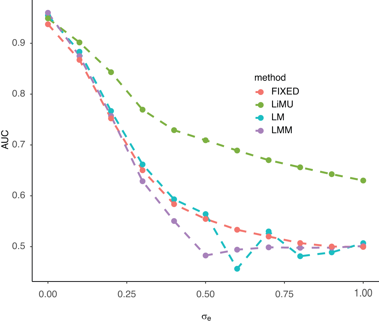
We propose a new LMM method for GWASs, using phylogenetic trees to control for population structure. We use Markov chain Monte Carlo (MCMC) to draw samples for the phylogeny based on observed genetic sequences, and then we compute the expected genetic similarity matrix induced by each phylogeny (Wang et al, 2021). We then apply the linear mixed model to each sampled expected genetic similarity matrix and average the results.

Simulations show that the true positive rates (TPRs) and FDRs of our method outperform both existing linear regression methods, LMM methods in which the genetic similarity matrix is estimated empirically, and pyseer with the genetic similarity matrix represented using consensus tree of MCMC posterior samples. We apply this method to MDR-TB in a GWAS of 467 TB subjects in a population from Lima, Peru (Grandjean et al, 2017).

2. METHODS

2.1. Linear mixed effects models for GWASs

We consider a population of samples typed at given single nucleotide polymorphisms (SNPs) and with measured phenotypes. We begin this section with an exposition of the linear mixed model (Kang et al, 2010; Lippert et al, 2011). Let the study subject indices be $i = 1, 2, \dots, N$ , and let the SNP locations be indexed by $m = 1, 2, \dots, M$ . Let $y = (y_{1}, y_{2}, \dots, y_{N})'$ denote a column vector of phenotypes ( $y_{i} \in ℛ$ ), and let $G = [G_{1}, G_{2}, \dots, G_{M}]$ denote genotype data observed at the M SNPs, with G_m denoting a column vector of alleles for the m-th SNP for all N subjects. For details on bacterial genetics, we refer readers to Earle et al (2016) and Coll et al (2014). Let $G_{i m} = 0$ and $G_{i m} = 1$ encode the events that subject i has the major allele or the minor allele at SNP m, respectively.

The LMM is a mixed effects model for association between SNP G_m and the phenotype. Independent LMMs may be applied at each SNP as follows: $y = G_{m} β_{m} + b_{m} + δ_{m} .$ (1)

Here $β_{m}$ is the effect size of the fixed effect of the m-th SNP, $δ_{m}$ is the random error vector, with $δ_{m} \sim M V N (0, σ_{g}^{2} I)$ , and $b_{m}$ is the random effect of the m-th SNP, with $b_{m} \sim M V N (0, σ_{e}^{2} ψ)$ , and $M V N (0, Σ)$ is the multivariate normal distribution with mean 0 and covariance $Σ$ . The genetic similarity matrix $ψ$ measures the genetic relatedness among different subjects. This is an $N \times N$ positive semidefinite matrix, and an empirical estimate of $ψ$ is given by Patterson et al (2006):

Here $μ_{m} = \frac{1}{N} \sum_{i = 1}^{N} G_{i m}, σ_{m}^{2} = μ_{m} (1 - μ_{m})$ are the empirical mean and variance (respectively) of the genotypes of the N subjects at the m-th SNP.

Although previous LMM study approximates $ψ$ by Equation (2), there is often uncertainty about the true value of $ψ$ . A realization of $ψ$ is implied deterministically by a phylogenetic tree for the N subjects (Wang et al, 2021). We denote this tree by t. In the next subsection we introduce a linear mixed model with uncertain genetic similarity matrix (LiMU), in which the genetic similarity matrix is unknown and is estimated based on the genotypes.

2.2. The LiMU method

The covariance matrix of the random effects for the m-th SNP is the positive-definite matrix $ψ$ , which measures the genetic relatedness among individuals. The empirical estimate of genetic similarity (shown in Equation 2) is inaccurate if genotypes are not densely sampled, or are of poor quality (Wang et al, 2021). The inaccuracy in empirical genetic similarity estimates may lead to inconsistent estimates for parameters in linear mixed models.

In this study, we propose a new linear mixed model for multivariate GWASs, by assuming an unknown genetic similarity matrix $ψ (t)$ that depends on the underlying phylogenetic tree t. Phylogenetics explicitly model a rate matrix, so branch lengths are likely to give a better estimate of genetic relatedness than the inner product of sequences used in existing software packages such as Genome-wide Efficient Mixed Model Association (GEMMA) (Zhou and Stephens, 2014).

Here we consider estimating the phylogeny t in a Bayesian framework. We place a proper prior distribution on the phylogenetic tree t (i.e., a uniform clock prior for a binary clock tree). After specifying the prior distributions, trees can be sampled conditioned on genotype data using standard software packages for phylogenetic inference (e.g., MrBayes; Ronquist et al 2012).

When multiple posterior samples of the phylogeny ${t_{j}}_{j = 1, \dots, J}$ are available (e.g., after running MrBayes for the phylogeny), we use the algorithm proposed in Wang et al (2021) to compute the expected genetic similarity matrix ${ψ (t_{j})}_{j = 1, \dots, J}$ for each posterior sample. The resulting matrices represent the uncertainty of genetic similarities among species, and we combine them with linear mixed models to account for population stratification and correct for spurious associations.

We associate each posterior sample ${ψ (t_{j})}_{j = 1, \dots, J}$ with a linear mixed model. For each j and m, we use restricted maximum likelihood (REML; Corbeil and Searle, 1976) to estimate parameters in each LMM $y = G_{m} β_{m j} + b_{m j} + δ_{m j} .$ (3)

Here $δ_{m j} \sim M V N (0, σ_{g}^{2} I)$ , $σ_{g}^{2}$ represents nongenetic variance due to nongenetic effects, and $b_{m j}$ is the random effect of the m-th SNP, and $ψ (t_{j})$ is the expected genetic similarity matrix, $b_{m j} \sim M V N (0, σ_{e}^{2} ψ (t_{j}))$ , $σ_{e}^{2}$ represents additive genetic variance. We compute the p value for ${\hat{β}}_{m j}$ , denoted by $p_{m j} = P (T_{m}^{r e p} > T_{m} | ψ (t_{j}))$ . Here T_m is the test statistic for site m, and it is a function of $ψ (t)$ . $T_{m}^{r e p}$ denotes the test statistic for a replication of site m. Finally, we compute the mean of p values $p_{m j}$ for each site m, $p_{m}^{*} = \frac{1}{J} \sum_{j = 1}^{J} p_{m j}$ .

We note that $p_{m}^{*}$ is a natural way to combine a set of p values since it is an unbiased estimator of $\int P (T_{m}^{r e p} > T_{m} | ψ (t)) π (ψ (t)) d ψ (t)$ . This is related to posterior predictive p values (Hjort et al, 2006; Meng, 1994). A permutation test is another option for finding p values for this test, and may be more precise than the mean, but we found that permutation tests are not computationally tractable with this model. Algorithm 1 provides an overview of the estimation procedure of LiMU. We provide an open-source software implementation for this method.^†

The computational cost for reconstructing a tree through MCMC is a linear function of $M \cdot N \cdot K$ . Here K is the number of MCMC samples. For each thinned posterior sample, the cost for computing the genetic similarity matrix is $O (N^{2})$ , and the cost for REML of LMM is $O (N^{3} \cdot M)$ . The wall time of these operations can be improved by parallelizing the REML step for each genetic similarity matrix computation.

For the experiments on TB data from peru, the sample collection and processing received ethical approval from the IRB of the Universidad Peruana Cayetano Heredia. In addition, the TB sequences are available through the European Nucleotide Archive (accession no: PRJEB5280) and are in the public domain.

3. EXPERIMENTS

3.1. Simulated data sets

3.1.1. Simulation 1

In the first simulation study, we simulated data sets for four scenarios: A, B, C, and D. The binary trees were simulated through the ms software (Hudson, 2002). We used the R package phangorn (Schliep, 2011) to create genetic variants under the assumption of the Jukes Cantor model (Jukes and Cantor, 1969). We assumed that the branch lengths are in units of $2 N$ generations. We standardized the genotypes (normalized to have mean 0 and variance 1), and uniformly chose one SNP to be significant for each data set. We computed a ground-truth genetic similarity matrix given the reference trees, according to Wang et al (2021).

We hypothesize that with a larger number of markers, the genetic similarity matrix will have less uncertainty, and LiMU results may approach those of the LMM. In scenario A: small data set, we simulated 50 trees with $N = 30$ taxa, each with $M = 500$ loci; In scenarios B: Genome-wide Complex Trait Analysis (GCTA) model, C: Illumina, and D: Nanopore, we simulated 50 trees with $N = 100$ taxa, each with $M = 2000$ loci. In scenarios A: small data set and B: GCTA model, we simulated the phenotype through the LMM described in Section 2.1, with $σ_{e} = 0.60$ , $σ_{g} = 0.50$ , effect size $β = 0.20$ , and with $σ_{e} = 0.40$ , $σ_{g} = 0.20$ , effect size $β = 0.20$ .

In scenarios C: Illumina, and D: Nanopore, we simulated the phenotype through the linear model (LM) with $σ_{e} = 0.20$ , $β = 0.20$ , genotyping error $0.5 %$ and $10 %$ , respectively. These two thresholds correspond to specific sequencing technologies used for tuberculosis (TB) genotyping, which determines which of relative few major types an isolate is. Based on estimates of error rates from different sequencing technologies, 0.5% is toward the higher estimate for most Illumina short read sequencing technologies (Stoler and Nekrutenko, 2021), and 10% is a good estimate for technologies with higher error rates, such as Oxford Nanopore sequencing (Nicholls et al, 2019), especially given the relatively high GC content (guanine-cytosine content) in Mtb (>60%), which can influence error rates (Delahaye and Nicolas, 2021).

We compared the TPR and FDR of LiMU, LMM (using the empirical genetic similarity matrix for the kinship), the fixed effects model with the genetic similarity matrix represented by MDS implemented in the pyseer software, a linear mixed effects model with the expected genetic similarity matrix computed from consensus tree of MrBayes (CLMM), and a linear model in a task in which associated genetic variants are recovered. To compute the similarity matrix of the model implemented in pyseer for controlling population structure, we used the consensus tree provided by MrBayes.

The estimation of linear mixed model was carried out using the efficient mixed model association (EMMA; Lippert et al 2011). For a fixed p value threshold $τ$ , we can compute the empirical number of false positive FP $_{τ}$ (an SNP is identified to be significant with a threshold $τ$ given the truth that it is not), and the empirical number of true positive TP $_{τ}$ (given the truth that an SNP is significant and it is identified with a threshold $τ$ ), for the 50 simulated data sets of each scenario. We examined the receiver operating characteristic (ROC) curves (plot the TPR vs. the false positive rate [FPR] as we vary $τ$ ) induced by the p values for these models for simulated data in which the ground truth is known.

Figure 1 displays the ROC found for these methods for data sets A: small data set (upper left panel), B: GCTA model (upper right panel), C: Illumina (middle left panel), and D: Nanopore (middle right panel). The lower panels show the partial ROC curves of the top left corner for scenarios B, C, and D. In scenarios A and B, the ROC curve of LiMU dominates those of pyseer, LMM, and LM at all FDR levels in both scenarios. In scenario C, the data were generated through a linear regression model, the ROC curves found for all methods were close. In scenario D, with higher genotyping error in data simulation, the area under all ROC curves was lower (compared with scenario C).

FIG. 1.

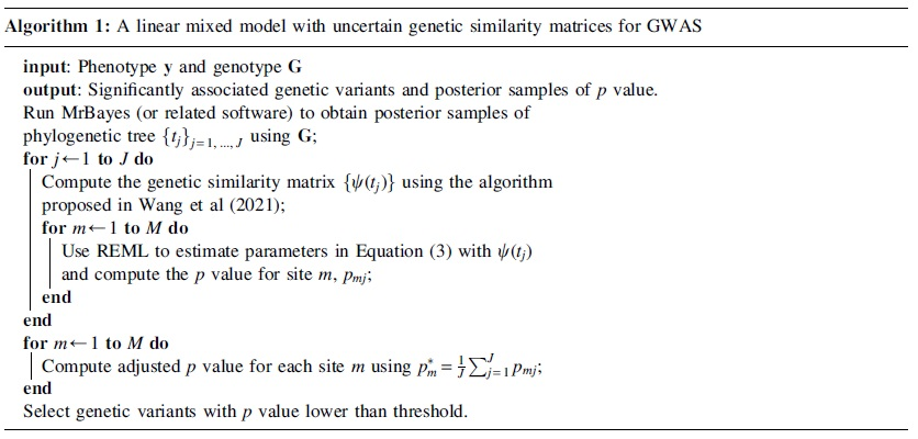
ROC provided by LM, LMM, the FIXED, a linear mixed effects model with the expected genetic similarity matrix computed using the consensus tree of MrBayes according to Wang et al (2021), and a LiMU for data sets (A): small data set (upper left panel), (B): GCTA model (upper right panel), (C): Illumina (middle left panel), (D): Nanopore (middle right panel), the vertical dotted line is at FPR level $0.05$ . The lower panels are partial ROC curves of the top left corner for scenarios B, C, and D. For scenario B, the LiMU model outperforms other methods at FPR level 0.05. CLMM, consensus linear mixed model; FIXED, fixed effects model implemented in the pyseer software; FPR, false positive rate; GCTA, Genome-wide Complex Trait Analysis; LiMU, linear mixed model with unknown genetic similarity matrices; LM, linear model; LMM, linear mixed model; ROC, receiver operating characteristic; TPR, true positive rate.

The area under the receiver operating characteristic (ROC) curve (AUC) and the improvement at FDR = 0.05 are listed in Table 1. Figure 2 shows the TPR at a fixed FDR level 0.05 for the four scenarios shown in Figure 1. The ROC curves provided by LiMU and LMM with the expected genetic similarity matrix computed from the consensus tree according to Wang et al (2021) exhibit similar performance.

FIG. 2.

TPR at a fixed FDR level $0.05$ for the four scenarios shown in Figure 1, detailing performance for a relevant FDR. FDR, false discovery rate.

Table 1.

AUC and True Positive Rate at False Discovery Rate 0.05 for Simulation Scenarios A, B, C, and D

Scenario	AUC					TPR (FDR = 0.05)
Scenario	LM	FIXED	LMM	LiMU	CLMM	LM	FIXED	LMM	LiMU	CLMM
A: Small data set	$0.706$	$0.703$	$0.713$	$0 . 760$	$0 . 760$	$0.24$	$0.20$	$0.26$	$0 . 32$	$0 . 32$
B: GCTA model	$0.958$	$0.958$	$0.980$	$0 . 992$	$0 . 992$	$0.78$	$0.82$	$0.92$	$0 . 98$	$0 . 98$
C: Illumina	$0.993$	$0.990$	$0 . 997$	$0.993$	$0.993$	$0 . 98$	$0.96$	$0 . 98$	$0 . 98$	$0 . 98$
D: Nanopore	$0 . 969$	$0.965$	$0.961$	$0.966$	$0.966$	$0 . 90$	$0.86$	$0 . 90$	$0 . 90$	$0 . 90$

LiMU shows improved AUC and TPR in scenarios A and B. The AUC and TPR are close for all methods in scenario C.

AUC, area under the ROC curve; CLMM, consensus linear mixed model; FDR, false discovery rate; FIXED, fixed effects model implemented in the pyseer software; GCTA, Genome-wide Complex Trait Analysis; LiMU, linear mixed model with uncertain genetic similarity matrix; LM, linear model; LMM, linear mixed model; TPR, true positive rate.

Bold indicates the best method (highest TPR or highest AUC).

3.1.2. Simulation 2

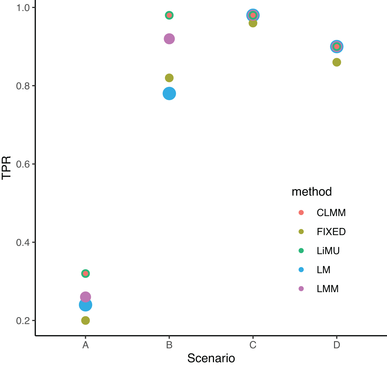
In the second simulation study, we first examined the area under the ROC curve (AUC) provided by the four methods already discussed as a function of $σ_{e}$ . We simulated 50 trees with $N = 15$ taxa, each with $M = 100$ loci. We considered 11 levels of $σ_{e}$ equally distanced between 0 and 1. For each level of $σ_{e}$ , we simulated the phenotype through the LMM described in Section 2.1, with $β = 0.1$ , $σ_{g} = 0.1$ . Hence, we have 50 data sets for each level of $σ_{e}$ . The rest of the setup for this simulation was the same as the previous simulation study.

We also report the compute time required for each step of LiMU in the first row of Table 3. The experiments were conducted on a 2.3 GHz Intel Core i9 processor. Half a million iterations of MrBayes run costs $6.524$ seconds, computation of the genetic similarity matrix for one thinned posterior sample takes $6.84 \cdot 1 0^{- 3}$ seconds, and one run of REML with a sample for the genetic similarity matrix takes $0.613$ seconds.

We examined the area under the ROC curves (AUC) induced by the p values of linear regression (LM), linear mixed model with empirical genetic similarity matrix (LMM), the pyseer software (pyseer) and a linear mixed model with unknown genetic similarity matrices (LiMU), for simulated data in which the ground truth was known. Figure 3 displays the area under curve (AUC) as a function of $σ_{e}$ . When $σ_{e}$ is small, the AUC provided by the four methods is similar. The AUCs of LiMU and rest of the methods start to diverge once we increase $σ_{e}$ , showing that LiMU outperforms the other methods significantly when the heritability is high.

FIG. 3.

AUC as a function of $σ_{e}$ provided by LM, LMM, the pyseer software (pyseer), and a LiMU. With a small value of $σ_{e}$ , the AUC provided by the four methods is close. LiMU and the other methods start to diverge once we increase $σ_{e}$ . LiMU works better with higher heritability $h^{2} = σ_{e}^{2} ∕ (σ_{e}^{2} + σ_{g}^{2})$ . AUC, area under curve.

In addition, we examined the area under curve (AUC) as a function of $σ_{e}$ provided by LiMU with p value summarized by four different statistics (max, mean, min, median). Figure 4 indicates that the AUC provided by mean and median statistics is similar, and is higher than max statistics with a high level of $σ_{e}$ , the AUC provided by the min statistic is lower than the other three.

FIG. 4.

AUC as a function of $σ_{e}$ provided by LiMU with p value summarized by four different statistics (i.e., max, mean, min, median). The AUC provided by mean and median statistics is close, and is higher than max statistics with a high level of $σ_{e}$ . The AUC provided by min statistic is lower than the other three.

3.1.3. Simulation 3

In the third simulation study, we design experiments with more sophisticated setups. We create 50 data sets, in each of them we randomly sample $N = 50$ genetic sequences among the 467 TB isolates that we analyzed in Section 3.2. We first run MrBayes to obtain a consensus phylogeny for each data set, and the expected genetic similarity matrix for the consensus tree is used to simulate phenotype. The amount of uncertainty in the phylogeny can be quantified using the R package treespace (Jombart et al, 2017; R Core Team, 2013).

Figure 5 shows the density plot for the first two components provided by metric MDS (Williams, 2000). The MDS is conducted on the pairwise distance between the 100 thinned posterior samples for one of the 50 data sets using treespace.

FIG. 5.

The density plot for the first two components provided by metric MDS. The MDS is conducted on the pairwise distance between the 100 thinned posterior samples for 1 of the 50 data sets using treespace. MDS, multidimensional scaling.

We investigate the effects of polygenic traits using LiMU, linear model (LM), linear mixed model with empirical genetic similarity matrix (LMM), and the fixed effects model implemented in the pyseer software (FIXED). The genetic sequences are obtained by randomly sampling M sites from the original TB sequences. We examine three levels of M, $M = 100, 300, 1000$ . For each level of M, we simulate phenotypes in four scenarios using multiple d significant loci, according to

where $δ_{j} \sim M V N (0, σ_{g}^{2} I)$ and $b_{j} \sim M V N (0, σ_{e}^{2} ψ (t_{j}))$ , with $σ_{g} = 0.2$ and $σ_{e} = 0.4$ . In each scenario we simulate 50 data sets with different random seeds. The number of significant loci is set to $d =$ 1, 2, 5, and 10 in the four scenarios, respectively. The effective sizes are sampled from uniform distribution $U (0, 0.3)$ for scenarios $d = 1, 2, 10$ , and are sampled from uniform distribution $U (0, 0.5)$ .

Figure 6 shows the AUC as a function of M provided by LiMU, linear model (LM), linear mixed model with empirical genetic similarity matrix (LMM), and the FIXED in four scenarios with size of effects 1 (upper left), 2 (upper right), 5 (lower left), and 10 (lower right). The AUCs provided by LMM and LiMU are higher than those provided by LM and FIXED. For all cases, LiMU approaches LMM with a higher value of M. For a small value of M, LiMU performs slightly better than LMM when there is only a single significant locus, and LMM performs better than LiMU when there are multiple significant loci.

FIG. 6.

AUC as a function of M provided by LiMU, LM, LMM, and the FIXED in four scenarios with number of significant loci d = 1 (upper left), 2 (upper right), 5 (lower left), and 10 (lower right).

3.2. Association study for MDR-TB in Lima, Peru

We carried out a GWAS using the LiMU method to control for population structure for 467 TB subjects (of which 158 had MDR strains) collected in Lima, Peru. These data were previously studied in Grandjean et al (2017), and in that study, many homoplastic variant sites were identified to be significantly correlated, indicating epistasis. Our analysis further refines these results with the LiMU control for population structure. We removed genotypes with minor allele frequency < $0.005$ , yielding 9848 SNPs.

We compared LM, the fixed effects model with the genetic similarity matrix represented by MDS implemented in software pyseer, LMM, and the LiMU. For the LMM, we use the empirical genetic similarity matrix, and the inference was carried out by the EMMA method. For LiMU, we first ran MrBayes to get posterior samples of trees. We ran MrBayes with 1 million iterations, with burn-in given by the first half of the chain, and we collected 50 thinned posterior tree samples. Given the expected genetic similarity matrix based on each sampled tree, we use the EMMA method to infer the LMM parameters.

The genetic similarity matrix of the fixed effects model in pyseer was computed using the consensus tree provided by the MrBayes analysis. We consider MDR as the phenotype of interest, and form a binary variable indicating MDR or non-MDR. All samples identified as resistant to either rifampicin or isoniazid (but not resistant to other drugs) are included in the non-MDR set.

We compared our methods with a classical linear regression GWAS with t-tests. This linear analysis identified 100 genetic variants that significantly associated with MDR after Bonferroni (BF) correction, with p value $< 0.05 ∕ 9848$ . The LiMU identifies 23 significantly associated genetic variants (red pluses in Fig. 8) after BF correction (p values $< 0.05 ∕ 9848$ ). LMM identifies eight associated genetic variants (blue triangles) after BF correction. Figure 7 shows a Venn diagram of base pair (BP) positions for hits provided by LMM and LiMU.

FIG. 7.

The base pair positions of LiMU and LMM hits. BP, base pair.

FIG. 8.

Manhattan plot of genome-wide association studies carried out by LM, the FIXED, linear mixed model (LMM), and LiMU for the TB data. The dashed horizontal line indicates the threshold after BF correction. The base pair positions of LiMU hits are also provided. BF, Bonferroni; TB, tuberculosis.

The fixed effects model implemented in pyseer software identifies 96 associated genetic variants (gray crosses) after BF correction. Both LMM and LiMU significantly correct hits found through linear regression, suggesting that many of these hits are due to population structure. Figure 8 displays the Manhattan plot for these GWASs. Table 2 gives the p values of the three most significant hits identified by LiMU. We also summarize the posterior p values through posterior median and geometric mean, yielding values that are close to the p values summarized by mean (the $- {log}_{10}$ p values found by posterior median and geometric mean match those found by the posterior mean to two decimal places).

Table 2.

Negative Log p Values of LM, LMM, LiMU, and pyseer for Base Pair Positions $761, 115$ , $761, 160$ , and $2, 155, 176$

BP position	$761, 115$	$761, 160$	$2, 155, 176$
LM	8.12	17.95	8.53
LMM	14.45	15.01	4.23
LiMU	7.92	17.51	8.06
pyseer	7.88	16.64	8.26

LM, linear model; LMM, linear mixed model; LiMU, linear mixed model with uncertain genetic similarity matrix; BP, base pair.

The second row of Table 3 reports the timing (in seconds) for the three main steps of LiMU (i.e., 1 million iterations of MrBayes, computation of the genetic similarity matrix, and REML for one LMM fit). One million iterations of MrBayes run costs $8414.99$ seconds, computation of the genetic similarity matrix for one thinned posterior sample takes $0.437$ seconds, and one run of REML takes $4799.37$ seconds.

Table 3.

Timing (in Seconds) of Each Step in LiMU for Simulation 2 (Row 1) and Real Analysis (Row 2)

	MrBayes	GSM	REML
$N = 15 ∕ M = 100$	$6.524$	$6.84 \cdot 1 0^{- 3}$	$0.613$
$N = 467 ∕ M = 9848$	$8414.99$	$0.437$	$4799.37$

The experiments were conducted on a 2.3 GHz Intel Core i9 processor.

LiMU, linear mixed model with uncertain genetic similarity matrix; GSM, genetic similarity matrix; REML, restricted maximum likelihood.

The hits with BP positions 761,160 and 761,115 are nonsynonymous mutations (these alter the amino acid produced) in the rpoB gene, which is associated with rifampin resistance (Goldstein, 2014; Lipin et al, 2007). The majority of mutations that confer resistance to rifampin occur within an 81 bp region of rpoB, referred to as the rifampin-resistance determining region (RRDR). And although neither of the sites identified here occur within the RRDR, there is still a chance that strains carrying these mutations may be rifampin resistant, or they may be compensatory mutations (Lempens et al, 2018; Ma et al, 2021).

In addition, the hit with BP position 2,155,176 is a nonsynonymous mutation in the katG gene, which is associated with isoniazid resistance. Rifampin and isoniazid are first-line antimicrobials used to treat TB and strains resistant to both are termed MDR-TB (Lipin et al, 2007).

There was also a hit identified by LiMU for a nonsynonymous mutation within rpoC, which has been previously shown be involved in compensation of fitness costs associated with rifampin resistance (De Vos et al, 2013). In addition, there were hits within various Pro-Pro-Glu (PPE) and Pro-Glu and polymorphic guanine-cytosine-rich repetitive sequence (PE-PGRS) family genes, and although the exact function of many of these genes is not well understood, there is evidence that many are involved in the host–pathogen interaction and infection (Qian et al, 2020). However, there can be technical challenges with assembly and variant calling at these loci because of a high GC content and excess of repetitive sequences (Ates, 2020), and further study would be required to validate the variation found in these genes.

4. DISCUSSION

Standard linear mixed models (LMMs) for GWASs often assume a single known genetic similarity matrix as a random effect (typically computed as the symmetric matrix resulting from inner products of genetic variants). However, such an approach is inaccurate if genotypes are not densely sampled, or are of poor quality (Wang et al, 2021): in Wang et al (2021), it was found that uncertainty in genetic similarity matrices (measured in standard deviation) varied from $0.223$ to $0.031$ as number of markers varied from 20 to 1000. Uncertainty about the genetic similarity matrix may degrade the quality of LMM estimates.

We have developed a linear mixed effects model for GWASs incorporating uncertainty about the genetic similarity matrices, in which the genetic similarity matrix is induced by a phylogeny based on the genotype. To account for the uncertainty of phylogeny, we considered a Bayesian framework for the underlying tree and derive the posterior samples through MCMC methods (i.e., MrBayes). Our proposed method, LiMU, is computationally more expensive than standard LMMs as we require multiple runs of standard LMM, and use Bayesian sampling methods to obtain posterior tree samples. However, LiMU allows us to consider the uncertainty in the genetic similarity matrix (or phylogeny).

In LiMU, we first estimate posterior samples for the phylogeny, and then estimate parameters of the LMM conditioned on the trees. Our method can utilize any Bayesian phylogenetic inference methods that exist in current literature (Bouckaert et al, 2014; Ronquist et al, 2012; Wang and Wang, 2021; Wang et al, 2020). In addition, our method is flexible in the sense that the estimates of phylogenies could be obtained from DNA, RNA, or any data source arising from trees (including phylolinguistic data, for example).

Our simulations demonstrate the consistency of our methods, and improved FPRs over the LMM and the fixed effects model implemented in pyseer software. The ROC curve and AUC provided by LiMU dominate those provided by the LMM, the fixed effects model implemented in pyseer software, and a linear model. Our simulations further show that the advantage of LiMU is seen most clearly when the heritability of the phenotype is high. There is more uncertainty in the phylogeny for smaller data sets, and in this case LiMU is preferable.

We also demonstrate that LiMU is robust to model misspecification and high genotyping error (LiMU outperforms other methods in simulations with high genotyping error, and with simulations in which the phenotypes are not sampled from an LMM). We recommend that LiMU be used for data sets with high genotyping error or small number of markers. Our experiments involved <10,000 markers. If the number of markers is much larger, then the genetic similarity matrix will have less uncertainty and LiMU results may approach those of the LMM.

We apply our method to a GWAS of 467 MDR-TB (with ∼10,000 markers) in a population from Lima, Peru. In our real data analysis, LiMU found fewer hits than a linear model without random effects. The hits we found involve nonsynonymous mutations in the rpoB and katG genes, and a nonsynonymous mutation within rpoC, that is associated with rifampin resistance. These genes are known to be involved with MDR or host–pathogen interaction and infection. Our simulations suggest that the FPR of LiMU is lower than that of the LMM, and so these hits are likely to be true positives. Also, the hit we identified at BP position 2,155,176 was not found by the LMM.

Our current approach is limited to sequences without recombination. We could extend to data with recombination events in genealogies. The ancestral recombination graph (ARG) describes the coalescence and recombination events among individuals (Rasmussen et al, 2014). The ARG is composed of a set of coalescent trees separated by break points. To compute expected genetic similarity matrix for samples given an ARG, we could first compute the expected genetic similarity matrices for each of the coalescent trees in the ARG, then compute weighted average for those expected genetic similarity matrices.

The weights would be proportional to the number of loci between each consecutive pair of break points. Finally, we could apply LiMU to this weighted set of trees, computing their expected genetic similarity matrices. In cases wherein reconstructing ARG is computationally too intensive (e.g., whole genome sequences), we could use methods such as Fastgear (Mostowy et al, 2017), Clonalframeml (Didelot and Wilson, 2015), and Gubbins (Croucher et al, 2015) to remove recombination from alignments before phylogenetic reconstruction.

Footnotes

AUTHORs' CONTRIBUTIONS

S.W. and S.G. contributed to methodology, formal analysis, software, writing—original draft, and writing—review and editing. B.S. contributed to writing—original draft and writing—review and editing. L.G. contributed to data curation. L.W. contributed to writing—review and editing. C.C. contributed to conceptualization and writing—review and editing. L.T.E. contributed to conceptualization, methodology, writing—original draft and writing—review and editing.

ACKNOWLEDGMENTS

We thank the associate editor and anonymous referees who provided helpful comments to this article.

AUTHOR DISCLOSURE STATEMENT

The authors declare they have no conflicting financial interests.

FUNDING INFORMATION

This research is supported by the National Natural Science Funds of China (Grant No. 12101333), the Natural Science Funds of Tianjin (Grant No. 21JCQNJC00050), the Shanghai Science and Technology Program (Grant No. 21010502500), the startup fund of ShanghaiTech University, and NSERC (Grant Nos. RGPIN/05484-2019, RGPIN/2019-06131, and DGECR/00118-2019). L.T.E. is supported by a Michael Smith Health Research BC Scholor Award.

References

Ates

LS.

New insights into the mycobacterial PE and PPE proteins provide a framework for future research. Mol Microbiol, 2020; 113(1):4–21; doi: 10.1111/mmi.14409

Bouckaert

, Heled

, Kühnert

, et al. BEAST 2: A software platform for Bayesian evolutionary analysis. PLoS Comput Biol, 2014; 10(4):e1003537; doi: 10.1371/journal.pcbi.1003537

Bycroft

, Freeman

, Petkova

, et al. The UK Biobank resource with deep phenotyping and genomic data. Nature, 2018; 562(7726):203–209; doi: 10.1038/s41586-018-0579-z

Coll

, McNerney

, Guerra-Assuncao

, et al. A robust SNP barcode for typing Mycobacterium tuberculosis complex strains. Nat Commun, 2014; 5:4812; doi: 10.1038/ncomms5812

Corbeil

, Searle

SR.

Restricted maximum likelihood (REML) estimation of variance components in the mixed model. Technometrics, 1976; 18(1):31–38.

Cordero

, Polz

MF.

Explaining microbial genomic diversity in light of evolutionary ecology. Nat Rev Microbiol, 2014; 12(4):263–273; doi: 10.1038/nrmicro3218

Croucher

, Page

, Connor

, et al. Rapid phylogenetic analysis of large samples of recombinant bacterial whole genome sequences using Gubbins. Nucleic Acids Res, 2015; 43(3):e15; doi: 10.1093/nar/gku1196

Dahl

, Iotchkova

, Baud

, et al. A multiple-phenotype imputation method for genetic studies. Nat Genet, 2016; 48(4):466–472; doi: 10.1038/ng.3513

Delahaye

, Nicolas

Sequencing DNA with nanopores: Troubles and biases. PLoS One, 2021; 16(10):e0257521; doi: 10.1371/journal.pone.0257521

10.

De Vos

, Müller

, Borrell

, et al. Putative compensatory mutations in the rpoC gene of rifampin-resistant Mycobacterium tuberculosis are associated with ongoing transmission. Antimicrob Agents Chemother, 2013; 57(2):827–832; doi: 10.1128/AAC.01541-12

11.

Didelot

, Wilson

DJ.

Clonalframeml: Efficient inference of recombination in whole bacterial genomes. PLoS Comput Biol, 2015; 11(2):e1004041; doi: 10.1371/journal.pcbi.1004041

12.

Earle

, Wu

C-H

, Charlesworth

, et al. Identifying lineage effects when controlling for population structure improves power in bacterial association studies. Nat Microbiol, 2016; 1(5):16041; doi: 10.1038/nmicrobiol.2016.41

13.

Goldstein

BP.

Resistance to rifampicin: A review. J Antibiot, 2014; 67(9):625–630; doi: 10.1038/ja.2014.107

14.

Grandjean

, Gilman

, Iwamoto

, et al. Convergent evolution and topologically disruptive polymorphisms among multidrug-resistant tuberculosis in Peru. PLoS One, 2017; 12(12):e0189838; doi: 10.1371/journal.pone.0189838

15.

Hjort

, Dahl

, Steinbakk

GH.

Post-processing posterior predictive p-values. J Am Stat Assoc, 2006; 101(475):1157–1174.

16.

Hudson

RR.

Generating samples under a Wright-Fisher neutral model. Bioinformatics, 2002; 18(2):337–338; doi: 10.1093/bioinformatics/18.2.337

17.

Jiang

, Zheng

, Fang

, et al. A generalized linear mixed model association tool for biobank-scale data. Nat Genet, 2021; 53(11):1616–1621; doi: 10.1038/s41588-021-00954-4

18.

Jombart

, Kendall

, Almagro-Garcia

, et al. treespace: Statistical exploration of landscapes of phylogenetic trees. Mol Ecol Resour, 2017; 17(6):1385–1392; doi: 10.1111/1755-0998.12676

19.

Jukes

, Cantor

CR.

Evolution of protein molecules. In: Mammalian Protein Metabolism, Volume 3. (Munro HN. ed.) Academic Press: New York; 1969; pp. 21–132.

20.

Kang

, Sul

, Service

, et al. Variance component model to account for sample structure in genome-wide association studies. Nat Genet, 2010; 42(4):348–354; doi: 10.1038/ng.548

21.

Kirkpatrick

, Ge

, Wang

Efficient computation of the kinship coefficients. Bioinformatics, 2019; 35(6):1002–1008; doi: 10.1093/bioinformatics/bty725

22.

Lees

, Galardini

, Bentley

, et al. pyseer: A comprehensive tool for microbial pangenome-wide association studies. Bioinformatics, 2018; 34(24):4310–4312; doi: 10.1093/bioinformatics/bty539

23.

Lempens

, Meehan

, Vandelannoote

, et al. Isoniazid resistance levels of Mycobacterium tuberculosis can largely be predicted by high-confidence resistance-conferring mutations. Sci Rep, 2018; 8(1):1–9; doi: 10.1038/s41598-018-21378-x

24.

Lipin

, Stepanshina

, Shemyakin

, et al. Association of specific mutations in katG, rpoB, rpsL and rrs genes with spoligotypes of multidrug-resistant Mycobacterium tuberculosis isolates in Russia. Clin Microbiol Infect, 2007; 13(6):620–626; doi: 10.1111/j.1469-0691.2007.01711.x

25.

Lippert

, Listgarten

, Liu

, et al. FaST linear mixed models for genome-wide association studies. Nat Methods, 2011; 8(10):833–835; doi: 10.1038/nmeth.1681

26.

Listgarten

, Lippert

, Heckerman

FaST-LMM-Select for addressing confounding from spatial structure and rare variants. Nat Genet, 2013; 45(5):470–471; doi: 10.1038/ng.2620

27.

Listgarten

, Lippert

, Kadie

, et al. Improved linear mixed models for genome-wide association studies. Nat Methods, 2012; 9(6):525–526; doi: 10.1038/nmeth.2037

28.

Loh

P-R

, Kichaev

, Gazal

, et al. Mixed-model association for biobank-scale datasets. Nat Genet, 2018; 50(7):906–908; doi: 10.1038/s41588-018-0144-6

29.

Loh

P-R

, Tucker

, Bulik-Sullivan

, et al. Efficient Bayesian mixed-model analysis increases association power in large cohorts. Nat Genet, 2015;(3):284–290; doi: 10.1038/ng.3190

30.

, Luo

, Ge

, et al. Compensatory effects of M. tuberculosis rpoB mutations outside the rifampicin resistance-determining region. Emerg Microb Infect, 2021; 10(1):743–752; doi: 10.1080/22221751.2021.1908096

31.

Meng

X-L.

Posterior predictive p-values. Ann Statist, 1994; 22(3):1142–1160; doi: 10.1214/aos/1176325622

32.

Mostowy

, Croucher

, Andam

, et al. Efficient inference of recent and ancestral recombination within bacterial populations. Mol Biol Evol, 2017; 34(5):1167–1182; doi: 10.1093/molbev/msx066

33.

Nicholls

, Quick

, Tang

, et al. Ultra-deep, long-read nanopore sequencing of mock microbial community standards. Gigascience, 2019; 8(5):giz043; doi: 10.1093/gigascience/giz043

34.

Novembre

, Johnson

, Bryc

, et al. Genes mirror geography within Europe. Nature, 2008; 456(7218):98–101; doi: 10.1038/nature07331

35.

Patterson

, Price

, Reich

Population structure and eigenanalysis. PLoS Genet, 2006; 2(12):e190; doi: 10.1371/journal.pgen.0020190

36.

Price

, Patterson

, Plenge

, et al. Principal components analysis corrects for stratification in genome-wide association studies. Nat Genet, 2006; 38(8):904–909; doi: 10.1038/ng1847

37.

Qian

, Chen

, Wang

, et al. Role of the PE/PPE family in host–pathogen interactions and prospects for anti-tuberculosis vaccine and diagnostic tool design. Front Cell Infect Microbiol, 2020; 10:743.

38.

Rasmussen

, Hubisz

, Gronau

, et al. Genome-wide inference of ancestral recombination graphs. PLoS Genet, 2014; 10(5):e1004342; doi: 10.1371/journal.pgen.1004342

39.

R Core Team. R: A Language and Environment for Statistical Computing. R Foundation for Statistical Computing; Vienna, Austria; 2013.

40.

Ronquist

, Teslenko

, van der Mark

, et al. MrBayes 3.2: Efficient Bayesian phylogenetic inference and model choice across a large model space. Syst Biol, 2012; 61:539–542; doi: 10.1093/sysbio/sys029

41.

Schliep

KP.

phangorn: Phylogenetic analysis in R. Bioinformatics, 2011; 27(4):592–593; doi: 10.1093/bioinformatics/btq706

42.

Stoler

, Nekrutenko

Sequencing error profiles of illumina sequencing instruments. NAR Genom Bioinform, 2021; 3(1):lqab019; doi: 10.1093/nargab/lqab019

43.

Sudlow

, Gallacher

, Allen

, et al. UK biobank: An open access resource for identifying the causes of a wide range of complex diseases of middle and old age. PLoS Med, 2015; 12(3):e1001779; doi: 10.1371/journal.pmed.1001779

44.

Wang

, Wang

, Bouchard-Côté

An annealed sequential Monte Carlo method for Bayesian phylogenetics. Syst Biol, 2020; 69(1):155–183; doi: 10.1093/sysbio/syz028

45.

Wang

, Ge

, Colijn

, et al. Estimating genetic similarity matrices using phylogenies. J Comput Biol, 2021; 28(6):587–600; doi: 10.1089/cmb.2020.0375

46.

Wang

, Wang

Particle Gibbs sampling for Bayesian phylogenetic inference. Bioinformatics, 2021; 37(5):642–649; doi: 10.1093/bioinformatics/btaa867

47.

Williams

On a connection between kernel PCA and metric multidimensional scaling. In: Proceeds of the 13th International Conference on Advances in Neural Information Processing Systems. Adv Neural Inform Process Syst, 2000; 13.

48.

Yang

, Lee

, Goddard

, et al. GCTA: A tool for genome-wide complex trait analysis. Am J Hum Genet, 2011; 88(1):76–82; doi: 10.1016/j.ajhg.2010.11.011

49.

Zhang

, Ersoz

, Lai

C-Q

, et al. Mixed linear model approach adapted for genome-wide association studies. Nat Genet, 2010; 42(4):355–360; doi: 10.1038/ng.546

50.

Zhou

, Stephens

Efficient multivariate linear mixed model algorithms for genome-wide association studies. Nat Methods, 2014; 11(4):407–409; doi: 10.1038/nmeth.2848