A Transfer Learning-Based Classification Model for Particle Pruning in Cryo-Electron Microscopy

Abstract

The cryo-electron microscopy (cryo-EM) single-particle analysis requires tens of thousands of particle projections to reveal structural information of macromolecular complexes. However, due to the low signal-to-noise ratio and the presence of high contrast artifacts and contaminants in the micrographs, the semiautomatic and fully automatic particle picking algorithms tend to suffer from high false-positive rates, which degrades the confidence of structure determination. In this study, we introduce PickerOptimizer (PO), a transfer learning-based classification neural network for particle pruning in cryo-EM, as an additional strategy to complement the current automated particle picking algorithms. To achieve high classification performance with minimal human intervention, we adopted two key strategies: (1) utilizing the transfer learning techniques to train the convolutional neural network, where the knowledge gained from public classification datasets is applied to the field of cryo-EM. (2) Designing a multiloss strategy, a combination of multiple loss functions, to guide the optimization of the network parameters. To reduce the domain shift between cryo-EM images and natural images for pretraining, we build the first image classification dataset for cryo-EM, which contains positive and negative samples collected from EMPIAR entries. The PO is tested on 14 public experimental datasets, achieving accuracy and F1 scores above 95% in most cases. Furthermore, three case studies are provided to verify the model performance by applying PO on problematic particle selections, showing that our algorithm achieved better or comparable performance compared with other particle pruning strategies.

1. INTRODUCTION

The cryo-electron microscopy (cryo-EM) single-particle analysis (SPA) is able to obtain three-dimensional structures of protein and macromolecular complexes at near-atomic resolution (Banerjee et al., 2016; Zhang et al., 2015a; Zhang et al., 2017b). However, the reconstruction of these high-resolution structures generally requires tens of thousands of single-particle projections, and the success of the high-precision calculation closely depends on the number and the quality of the picked particles. However, manual picking is cumbersome and time-consuming, and may introduce manual bias into the procedure. To quickly collect a massive number of particles, many automatic particle picking algorithms (Wang et al., 2016; Bepler et al., 2019; Wagner et al., 2019) have been proposed to be an indispensable step in SPA workflows.

However, due to the problems intrinsic to the cryo-EM, such as the extremely low signal-to-noise ratio, the presence of contamination, and other artifacts, these particle picking methods suffer from high false-positive rates, typically ranging from 10% to more than 25% (Zhu et al., 2004; Li et al., 2021; Li et al., 2022). As a consequence, it is common practice in the field of cryo-EM to perform several preprocessing or postprocessing steps to clean and remove incorrectly picked particles.

Actually, there is already some work to distinguish the correctness of selected particles and complement particle pickers. One such method is Deep Consensus (Sanchez-Garcia et al., 2018), which calculates a smart consensus over the output of different particle picking algorithms, resulting in a set of particles with a lower false-positive ratio than the initial set obtained by the pickers. In this algorithm, as least two particle pickers are required to provide particle selection results, which is time-consuming and laborious.

Moreover, to gain a sufficiently accurate consensus, the accuracy of at least one particle picker needs to be guaranteed. Sanchez-Garcia et al. (2020) provide a more easy-to-use and fully automated solution, MicrographCleaner (MC), which is a deep learning package designed to perform a pixel-wise classification of micrographs to discriminate which region is suitable for particle picking, and those which are not. By providing a general model trained on a dataset of 539 manually segmented micrographs, the MC is able to work in a fully automated manner.

However, the capabilities of the algorithm are limited to the size and diversity of the training set, and the robustness of MC depends on the consistency of the training dataset and the new dataset. Since the cryo-EM imaging principle is rather complicated, the collection of micrographs may be affected by various factors such as biological samples, ice thickness, under-focus value, and other factors, making the data under different imaging conditions vary widely. In case large discrepancies exist between the new data and the training data, the MC may perform poorly.

In response to these challenges, we hope to provide a model that is familiar with the basic features of micrographs and can be quickly adapted to the characteristics of new dataset with minimal human intervention. In this study, we introduce PickerOptimizer (PO), a deep learning-based particle pruning algorithm that classifies the preliminarily selected particles into true-positive particles and false-positive particles. To achieve high classification performance with minimal training data, we adopt two techniques: (1) transfer learning technique. The convolutional neural network (CNN) of PO is trained utilizing the transfer learning techniques where knowledge from a large-scale natural image-classification task is leveraged to obtain image feature extraction ability.

Considering the huge discrepancy between cryo-EM images and natural images, we constructed an image classification dataset for cryo-EM, which contains positive samples (particles) and negative samples (carbon region and high-contrast contaminations) collected from EMPIAR (Iudin et al., 2016) entries. Therefore, the CNN is first pretrained with a combination of a natural image dataset and a cryo-EM image dataset, and then fine-tuned with only a few manually labeled samples from the new dataset to adapt to new features. (2) Multiloss strategy. To alleviate the overfitting problem caused by the small amount of training data and further improve the classification performance, we design a multiloss strategy for PO, where a combination of loss functions simultaneously guide the updating of model parameters.

To prove the performance of our method, we tested PO on several well-known public datasets, achieving accuracy and F1 score above 95% in most cases. We further verify the PO on three use cases, which demonstrated that (1) when compared with the commonly used particle postprocessing algorithm, MC, PO achieved better or equivalent performance on tackling different types of pollution. (2) PO is able to improve conventional particle pickers and complement deep learning-based ones where the particle optimization effect brought by applying stricter thresholds to these particle picking algorithms incurs non-negligible harm to the true particles.

Conversely, PO can mask out most wrongly picked false-positive particles with true-positive ones not being ruled out. (3) Compared with the commonly used particle analysis and selection step in the SPA analysis process, two-dimensional (2D) classification, PO is able to distinguish and remove more false-positive particles. The source code, pretrained models, and datasets are available at https://github.com/LiHongjia-ict/PickerOptimizer/.

2. METHODS

2.1. Algorithm

Figure 1A shows the overall architecture of PO, where the neural network mainly consists of two parts: a feature extractor and a classifier. The feature extractor comprises several layers, including convolution, max-pooling (MaxPooling), and N consecutive residual blocks (ResBlock). The classifier contains two branches that work for multiloss strategy (illustrated in subsubsecion 2.1.3), the first branch is composed of a global average (GAP) layer and a fully connected layer, and the other branch has an extra $1 * 1$ convolutional layer before the GAP layer to compress the number of channels of feature maps and enhance nonlinearity.

FIG. 1.

The overall architecture of PO. (A) The model framework of PO, including feature extractor and classifier. (B) The detailed components of the ResBlock. (C) The detailed information of the classifier. (D) The GAP pooling. GAP, global average; PO, pickerOptimizer; ResBlock, residual blocks.

For a given input sample, represented as a 2D array of $R^{n \times n}$ , after passing through the first shallow convolutional layer, MaxPooling layer, and a series of ResBlock, the input patch will be converted into a patch of highly abstract feature maps for final classification. The classifier is able to map the feature maps to a categorical vector that shows the probabilities assigned to each class.

In this work, the neural network is trained utilizing transfer learning techniques. First, the entire model is trained on a large dataset that is composed of natural and cryo-EM datasets to obtain a pretrained model, which maintains powerful feature extraction capabilities. When given a new dataset, the feature extractor part of the model is initialized with the weights of the pretrained model. The weight of the pretrained classifier will be directly discarded, and the weights of the fully connected layer will be randomly initialized to a uniform distribution. The whole model will then be fine-tuned with the new dataset to learn characteristics specific to this dataset. It is worth noting that the multiloss strategy is designed to alleviate the overfitting problem caused by the limited training dataset. Therefore, the classifier of the model for pretraining only contains the first branch, and the complete classifier is used for fine-tuning.

2.1.1. Residual blocks

In PO, the ResBlock are adopted to construct the basic feature extractor. The ResBlock are skip-connection blocks that learn residual functions with reference to the layer inputs, instead of learning unreferenced functions (He et al., 2016). Figure 2 illustrates the architecture of the original “plain” layer and the ResBlock. It can be found that, in “plain” layers, the feature map $H_{l - 1}$ is directly fed to two convolutional layers to fit the mapping function $g_{l} (\cdot)$ and calculate the H_l.

FIG. 2.

The illustration of (a) the “Plain” layer and (b) the ResBlock.

However, in the ResBlock, instead of hoping every few stacked layers directly fit a desired underlying mapping, we explicitly let these layers fit a residual mapping. As the Eq. (2) shows, denoting the desired underlying mapping as $H_{l} (\cdot)$ , the stacked nonlinear layers are designed to fit another mapping of $f_{l} (H_{l - 1}) : = H_{l} - i d (H_{l - 1})$ . The original mapping is recast into $f_{l} (H_{l - 1}) + i d (H_{l - 1})$ . The introduction of ResBlock removes the influence of the main part, thus accentuating minor changes. The detailed information of the ResBlock is shown in Figure 1B. $H_{l} = g_{l} (H_{l - 1})$ (1)

H_{l} = i d (H_{l - 1}) + f_{l} (H_{l - 1})

(2)

In Eq. (1), $H_{l - 1}$ indicates the feature map of ${(l - 1)}^{t h}$ layer, H_l indicates the feature map of $l^{t h}$ layer, and $g_{l} (\cdot)$ indicates the mapping function. In Eq. (2), $H_{l - 1}$ indicates the feature map of ${(l - 1)}^{t h}$ layer, H_l indicates the feature map of $l^{t h}$ layer, $f_{l} (\cdot)$ indicates the mapping function, and the $i d (\cdot)$ indicates identify mapping. He et al. (2016) proposed the hypothesis that it is easier to optimize the residual mapping than to optimize the original, unreferenced mapping. The ResBlock has been used in various tasks and has achieved significant performance (Kim et al., 2016; Song et al., 2017; Zhang et al., 2017a; Wu et al., 2018).

2.1.2. GAP pooling

To increase the nonlinearly of the feature maps, traditional CNN always contains multiple fully connected layers to construct the classifier. However, the FC layer covers most of the parameters of the network, which can easily cause model overfitting (Gao et al., 2021). In particular, our method strives to train the model with minimal data, causing a higher risk of overfitting. Therefore, to reduce model parameters and suppress overfitting, GAP pooling is introduced to replace the first FC layer. Moreover, there is no need for parameter optimization in the GAP pooling, which greatly reduces the computation complexity.

As shown in Figure 1C, the input of the classifier is a K high-dimensional feature map. After passing through a GAP pooling layer, each $k^{t h}$ input feature map $f_{k} (x, y)$ is compressed into a point (as shown in Fig. 1D). These points are then mapped to a category vector by the fully connected layer with a learned parameter matrix. Each element in the output vector is a real-valued confidence-rated prediction related to a class, and the input is assigned to the class with the highest probability. To compare the parameter scales of GAP and FC, suppose the input of the classifier are N feature maps with size $7 * 7$ , and the output is a $1 * 3$ category vector. Compared with a traditional classifier with only one FC layer, the parameters are reduced from $N * 7 * 7 * 1 * 3 = 147 * N$ to $N * 1 * 3 = 3 * N$ .

2.1.3. Multiloss strategy

The most serious problem caused by training the model with limited data is overfitting. To alleviate the overfitting problem, we propose a multiloss strategy for PO. The multiloss strategy was originally designed for multitask experiments, which works by adding auxiliary tasks to assist the main task to learn more information, thereby improving the performance of the main task. The different loss functions are designed for multiple tasks and the model parameters are optimized by sharing the loss gradients generated from different loss functions.

Therefore, the auxiliary task is able to bring a certain regularization effect to the main task and prevent the algorithm from overfitting to a single loss function. Since the design concept of this strategy coincides with the puzzle of our task, we adopted the idea of multiloss functions. To design the multiloss strategy specific to our work, two problems need to be solved, one is how to design multiple tasks, and the other is how to balance the weights among different tasks.

In our algorithm, designing other tasks seems redundant. To concisely split a single classification task into multiple tasks, we designed a new classifier as shown in Figure 1C. Compared with the ordinary classifier that contains only one branch to directly transform the feature map obtained from feature extractor to a category vector, we add a new branch to compress the dimension of the feature maps to half of the previous size using a 1*1 convolutional layer. The feature maps are optimized on two branches, respectively, and the generated gradients jointly update the network. In this way, a classification task is split into two tasks with the same goal. The two tasks are completely complementary and recursive, and there will be no conflict between the two tasks, thus conducive to our training optimization.

To find the optimal weights for different tasks, two rules need to be followed: different loss should be kept in the same order of magnitude, and the importance of the task should be reflected in the weight assigned to the task. First of all, to prevent the value of a loss function from ruling the entire loss result, and other loss functions being submerged, the magnitude of the loss value generated by different tasks needs to be at one level. Otherwise, the multitask design will be infinitely close to the experiment of a single task, and the effect of other tasks will not be reflected. Second, in the same order of magnitude, different weights should be assigned according to the importance of different loss functions. The final ratio needs to be decided according to the actual experimental condition. In our work, the multiloss function is designed as follows:

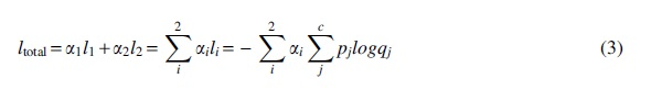
In the Eq. (3), $α$ is the hyperparameter, p is the real sample distribution, q is the predicted sample distribution, and c is the number of categories.

This strategy can not only optimize the classification performance but also bring a regularization effect to the model. According to the above description, the two tasks are two recursions of the same task and are complementary to each other. The hypothesis spaces generated by the two tasks are respectively denoted as $ℋ_{1}$ and $ℋ_{2}$ . Due to the recursive logic, $ℋ_{1} \subset ℋ_{2}$ and $ℋ_{1} \cap ℋ_{2} = ℋ_{1}$ are satisfied. Therefore, when $ℋ_{2}$ is updated, $ℋ_{1}$ is also updated. Since the hypothesis space $ℋ_{1}$ is updated by two tasks at the same time, $ℋ_{1}$ is more robust than $ℋ_{2}$ . Therefore, the classification results produced by the first branch are regarded as the results of the entire model, and the second branch only works for model parameter update.

2.2. Classification datasets

In this work, to familiarize the algorithm with the basic characteristics of images and enable the model to be quickly adapted to the characteristics of new cryo-EM images, the training data for the pretrained model come from two sources, natural images and cryo-EM images. For the natural one, we chose one of the most widely used large-scale datasets for benchmarking image classification algorithms, ImageNet (Deng et al., 2009) here. The dataset contains about 1.2 million images and is divided into 1000 categories, enabling the pretrained model to maintain powerful feature extraction ability.

However, considering the huge domain shift between the natural image and the cryo-EM micrographs, we constructed a cryo-EM dataset for image classification to enable the model to learn the image features specific to cryo-EM. The dataset contains positive samples (particles) and negative samples (carbon or ice-contaminated regions) manually selected from 14 different EMPIAR entries, as shown in Table 1. The whole dataset contains 3600 images and is divided into 36 categories (14 kinds of particles, 14 kinds of high-contrast contaminants, and 8 kinds of carbon regions) with 100 images in each category. The Figure 3 shows several samples selected from cryo-EM datasets.

FIG. 3.

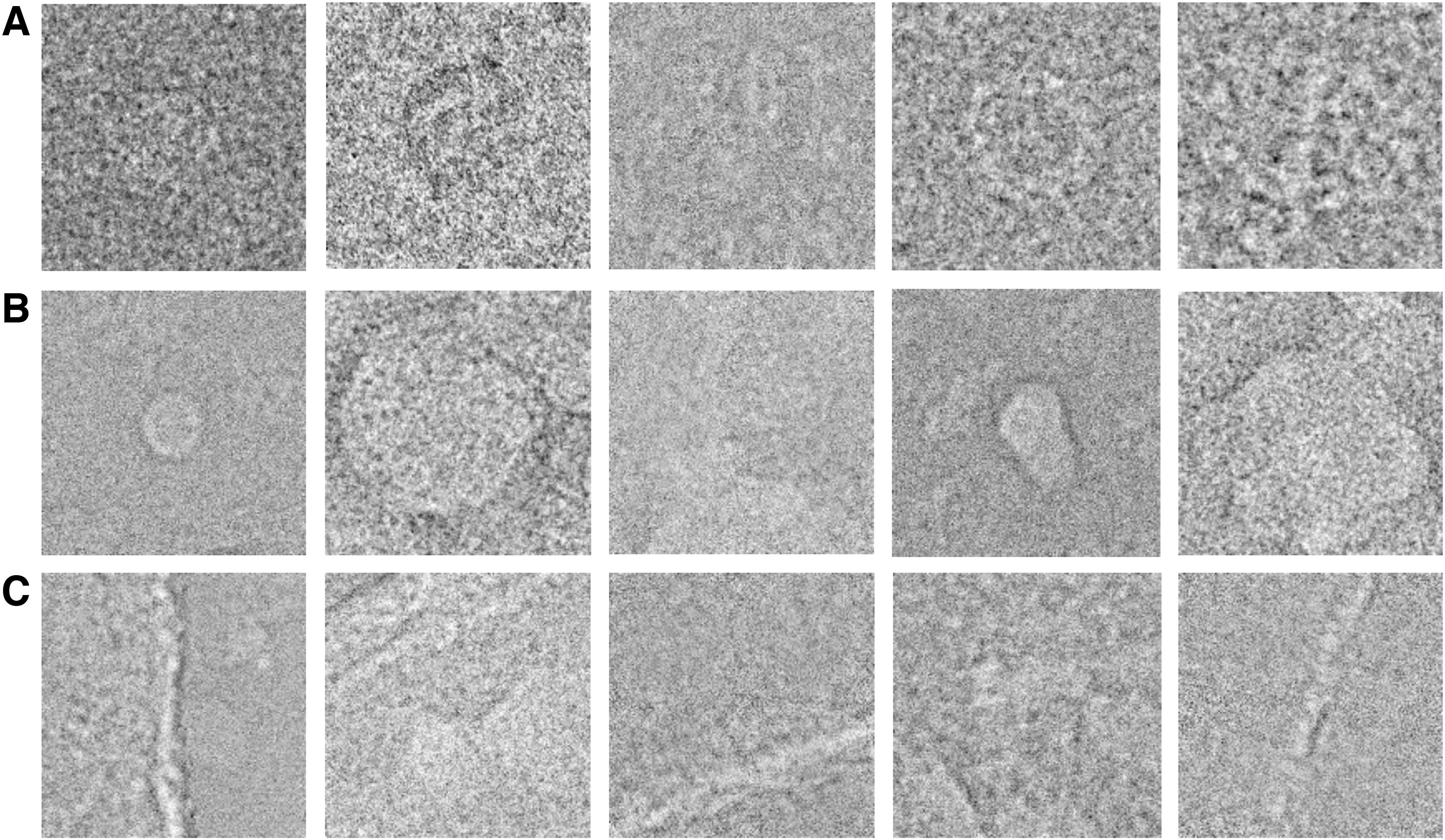
Examples of three different kinds of samples selected from the constructed cryo-EM datasets. (A) Examples of particles. (B) Examples of ice contaminants. (C) Examples of carbon regions. cryo-EM, cryo-electron microscopy.

Table 1.

The Detailed Information of the 14 Public Datasets in Cryo-Electron Microscopy Datasets

Dataset	Biological structure	Reference
EMPIAR-10406	70S ribosome	Nicholson et al. (2020)
EMPIAR-10059	NCP-CHD4 complexes	Gao et al. (2016)
EMPIAR-10285	P-Rex1G-beta-gamma signaling scaffold	Cash et al. (2019)
EMPIAR-10333	Human FACT	Liu et al. (2020)
EMPIAR-10590	human BAF complex	Mashtalir et al. (2020)
EMPIAR-10283	mammalian ATP synthase tetramer	Gu et al. (2019)
EMPIAR-10454	Saccharomyces cerevisiae fatty acid synthase complex	Singh et al. (2020)
EMPIAR-10470	Saccharomyces cerevisiae fatty acid synthase complex	Singh et al. (2020)
EMPIAR-10099	Hrd1 and Hrd3 complex	Schoebel et al. (2017)
EMPIAR-10350	LetB from Escherichia coli	Isom et al. (2020)
EMPIAR-10399	Arabinofuranosyltransferase AftD	Tan et al. (2020)
EMPIAR-10063	Activated NAIP2/NLRC4 Inflammasome	Zhang et al. (2015b)
EMPIAR-10097	Influenza Hemagglutinin Trimer	Tan et al. (2017)
EMPIAR-10077	Elongation factor SelB	Fischer et al. (2016)

With the rich information provided by the combination of ImageNet and cryo-EM dataset for pretraining, the algorithm can quickly learn the new features and obtain the capability to rule out false-positive particles from all picked particles in the new dataset.

2.3. Evaluation metrics

To quantify assess the performance of PO, we chose two metrics: accuracy and F1 score. As shown in Eq. (4), the accuracy refers to the percentage of all correctly classified observations to the total observations, which is the most intuitive indicator of the classification ability. The F1 score is the harmonic mean of precision and recall. Considering that the F1 score is only suitable for binary classification, but our task may be a triple classification task, we chose the macro-F1 score as the metric that weighs the F1 achieved on each label equally, as shown in Eqs. (5) and (6). $A c c u r a c y = \frac{T N + T P}{T N + F N + T P + F P}$ (4) $F 1 = \frac{2 \times p r e c i s i o n \times r e c a l l}{p r e c i s i o n + r e c a l l} = \frac{2 T P}{2 T P + F N + F P}$ (5)

In Eqs. (4) and (5), $T P$ means true positive, $T N$ means true negative, $F N$ means false negative, and $F P$ means false positive. In Eq. (6), N indicates the number of categories and $F 1_{i}$ indicates F1 score achieved on the $i^{t h}$ category.

3. EXPERIMENTS AND RESULTS

3.1. Data preparation

As described in subsection 2.2, 14 public cryo-EM datasets collected from EMPIAR together with the natural datasets ImageNet are used for model pretraining. These cryo-EM datasets are also used to evaluate the performance of PO. To avoid crossover between the dataset for pretraining and training, in the Results section, the datasets for pretraining only contain 13 datasets from Table 1, and the remaining one dataset is used for model training (fine-tuning) and evaluation. For example, to obtain the classification model for EMPIAR-10406, the ImageNet and the whole cryo-EM datasets, except EMPIAR-10406, are used for pretraining. Then the data randomly sampled from EMPIAR-10406 are used for model fine-tuning.

3.2. Training details

The training of PO consists of two steps: model pretraining and model fine-tuning. All the neural networks in this work are implemented with Pytorch (Paszke et al., 2019).

First, the model is pretrained with a combination of ImageNet and cryo-EM datasets. In our work, for simplicity, the feature extractor of the classification neural network is initialized with the pretrained weights of the resnet provided by PyTorch. In this way, the network is able to be familiar with the characteristics of natural images and some basic features of images, such as edges and corners. On this basis, the fully connected layer is freshly initialized and the entire model is fine-tuned with the constructed cryo-EM datasets to master the characteristics of the cryo-EM data.

The network is trained for 200 epochs on one 2080TI GPU with a batch size of 256. According to the training experience, we used stochastic gradient descent (SGD) (Bottou, 2012) with momentum as the optimizer, and the learning rate is initialized as 0.1. The momentum is set as 0.9. The MultiStageLR descent strategy is adopted to gradually converge the model where the learning rate is scaled down by a factor of 0.1 after every 7 epochs.

The fine-tuning of the network with the new dataset is carried out for 30 epochs on one 2080TI GPU with a batch size of 24. The learning rate is initialized as 0.01 and the MultiStageLR descent strategy is adopted here where the learning rate is scaled down by a factor of 0.1 after every 7 epochs. The same SGD with momentum as pretraining is adopted. The network is expected to be fine-tuned with minimal training samples. Therefore, to avoid the bias caused by the randomness of sampling, we sample the dataset multiple times (about 10,000 times) and train multiple models. The averaged macro-F1 score and accuracy of these models are considered the overall metrics of the model.

To suppress overfitting, we adopted several data augmentation strategies, including random horizontal flip, random vertical flip, and random rotation.

3.3. Performance of PO

3.3.1. Classification performance

We evaluate the classification performance of PO on 14 public datasets. Since our method strives to use minimal data to train the model, the network is tested with different amounts of training data. We constructed three kinds of dataset, denoted 10 shots, 20 shots, and 30 shots, which corresponds to 10, 20, and 30 samples in each category, respectively. For training a deep convolutional network, the amount of data in these three datasets is far from meeting data demands.

Table 2 shows the related metrics on different datasets, including macro-F1 score and accuracy. It can be found that the PO is able to achieve the macro-F1 score and accuracy of more than 95% in most cases. It demonstrates that the particle pruning algorithm is able to accurately judge whether the particle is true positive. Even in extremely difficult cases, such as EMPAIR-10454 and EMPAIR-10470, when the amount of training data reaches 30 shots, the classification metrics can approach about 90%. Moreover, it can be seen that the addition of training data not only improves the classification performance of the network but also increases the stability of the model, since a larger amount of training data brings a smaller variance of the classification metrics.

Table 2.

The Classification Performance (Macro-F1 Score and Accuracy) of PickerOptimizer on Different Datasets

	F1 score (%)			Accuracy (%)
	10 shots	20 shots	30 shots	10 shots	20 shots	30 shots
10406	92.08 ± 3.37	95.09 ± 1.83	96.13 ± 1.44	94.48 ± 2.27	96.39 ± 1.27	97.07 ± 1.11
10059	97.02 ± 1.65	98.00 ± 0.98	98.59 ± 0.94	97.70 ± 1.43	98.36 ± 0.89	98.94 ± 0.75
10285	98.03 ± 1.85	98.87 ± 1.14	99.31 ± 0.77	98.62 ± 1.50	99.13 ± 0.94	99.51 ± 0.69
10333	98.10 ± 1.80	99.17 ± 1.10	99.46 ± 0.69	98.54 ± 1.50	99.35 ± 0.99	99.67 ± 0.55
10590	99.05 ± 0.79	99.33 ± 0.42	99.41 ± 0.48	99.50 ± 0.54	99.67 ± 0.32	99.67 ± 0.36
10283	96.43 ± 1.67	97.36 ± 1.02	97.46 ± 1.08	97.04 ± 1.39	97.57 ± 0.96	97.89 ± 0.94
10454	76.58 ± 4.98	84.24 ± 3.40	87.70 ± 2.69	79.42 ± 4.36	86.35 ± 3.09	88.96 ± 2.45
10470	79.18 ± 4.33	86.25 ± 2.86	89.28 ± 2.46	82.26 ± 3.76	87.72 ± 2.55	89.96 ± 2.26
10099	97.02 ± 2.01	98.26 ± 1.62	98.57 ± 1.14	98.31 ± 1.10	98.98 ± 0.78	99.18 ± 0.73
10350	96.36 ± 2.73	98.26 ± 1.71	98.80 ± 1.35	98.20 ± 1.47	99.04 ± 1.06	99.38 ± 0.84
10399	97.47 ± 1.72	98.36 ± 1.39	98.77 ± 1.19	98.66 ± 1.11	99.20 ± 0.80	99.40 ± 0.75
10063	98.43 ± 1.25	98.67 ± 1.17	98.96 ± 0.93	99.19 ± 0.81	99.43 ± 0.67	99.59 ± 0.59
10097	95.01 ± 2.73	96.84 ± 1.88	97.72 ± 1.65	96.20 ± 1.96	97.82 ± 1.35	98.63 ± 1.17
10077	95.98 ± 1.96	96.76 ± 1.96	96.93 ± 1.83	97.12 ± 1.44	97.59 ± 1.39	97.94 ± 1.24

Notes: 10 shots, 20 shots, and 30 shots corresponds to 10, 20, and 30 samples in each category of training dataset.

3.3.2. Use cases

To intuitively reveal the optimization effect of PO on particle selections, in this section, we provide three case studies, where the particle pickers struggle to identify particles from problematic regions (carbon areas and high-contrast contaminations), and thus they all could benefit from PO. The classification neural network trained with “30 shots” is adopted as models for PO.

3.3.2.1. Comparison with other pruning approaches

The PO is compared with MC, which performs particle postprocessing by discriminating the desirable and undesirable regions for particle picking. It is one of the most frequently adopted particle postprocessing algorithm for cryo-EM. The Relion Autopicker (RA) (Scheres, 2012; Scheres, 2015) is chosen as the representative particle picker to generate the preliminary selection of particles. There are three possible scenarios for pollutants in a micrograph as shown in Figure 4, where the first case contains a large carbon region in the micrograph, the second case contains various ice contaminants to interfere with the particle picking, and the third case contains the presence of both. We tested PO on all three cases. Figure 4 shows the particles picked by RA (the first row), the remaining particles after applying MicrographCleaner (the second row), and PO (the last row).

FIG. 4.

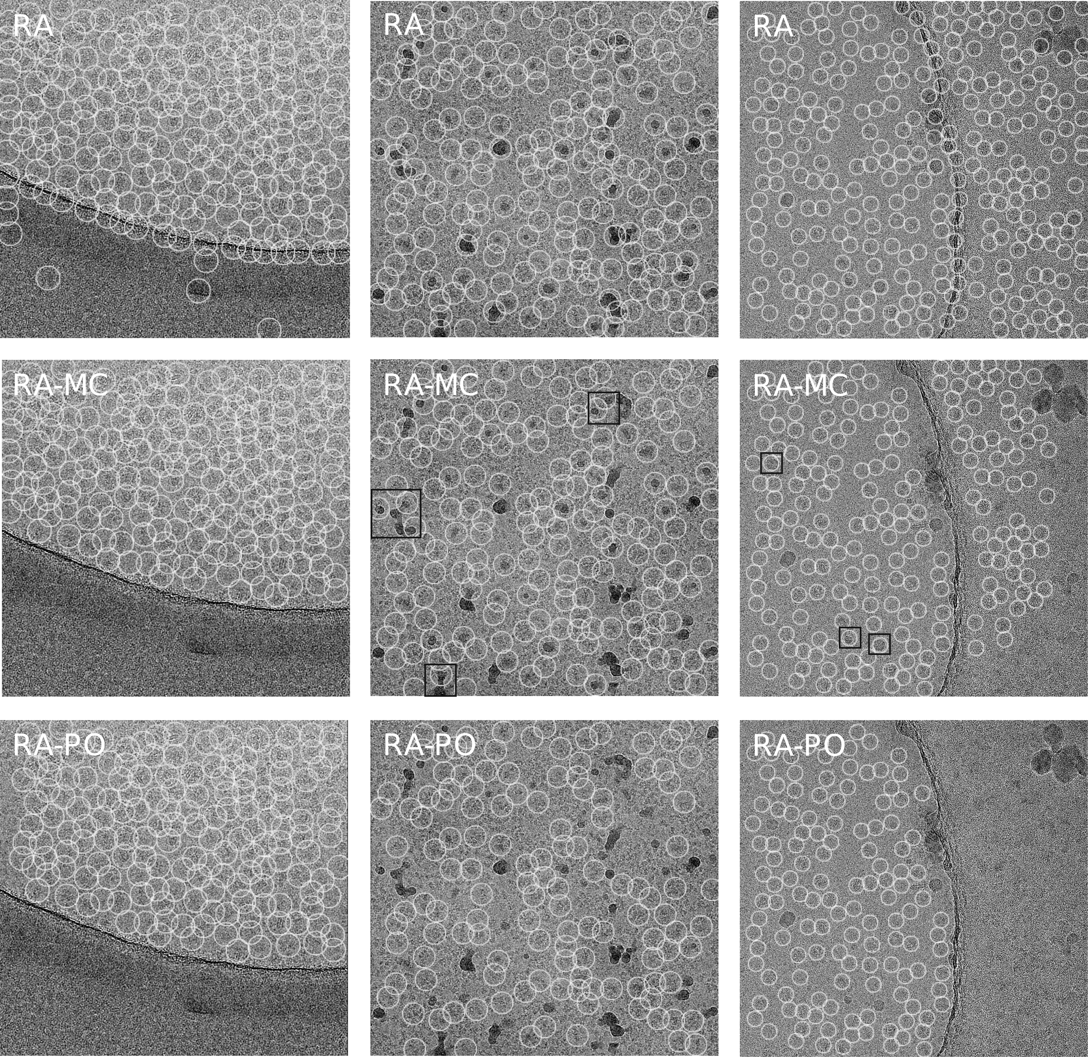
The comparison of MC and PO on dealing with different types of pollutants, including carbon (the first column), ice-contaminated areas (the second column), and both (the third column). The first row corresponds to particles picked by RA, the second row corresponds to the RA-MC, and the last row corresponds to the RA-PO. MC, MicrographCleaner; RA, Relion autopicker; RA-MC, remaining particles after applying MicrographCleaner; RA-PO, remaining particles after applying pickerOptimizer.

In all these three challenging cases, the RA tends to erroneously pick up a lot of false-positive particles in ice-contaminated and carbon regions; thus, further optimization is required. In the case where only carbon region exists (the first column in Fig. 4), both MC and PO performed excellently and can perfectly avoid the particle picked in the carbon region, with true-positive particles not being ruled out. However, when tackling the presence of a large amount of ice pollution in a micrograph (the second column in Fig. 4), the performance of MC decreased significantly.

Although most negative samples are filtered out, there is still some obvious ice pollution left. Conversely, PO is able to identify and rule out almost all contaminations and nearby affected particles. Likewise, in the third case where the carbon area is relatively indistinguishable from the normal area, the performance of MC is even worse, where the wrongly selected ice contaminants and particles in carbon areas are left, although applying MC. Obviously, our method can avoid particle picking in ice-contaminated and carbon areas more accurately. In this study, the recommended default threshold of 0.2 is used in all experiments of MC.

3.3.2.2. Comparison with the thresholding of particle pickers

Many particle picking algorithms have provided an adjustable threshold when calculating the selected particles, which reflects the confidence of the particles. This is a particle optimization trick provided by the particle picker itself and is very convenient to use. In this study, we compared PO with Topaz and the crYOLO (Wagner et al., 2019) particle pickers, which are representative pickers providing a threshold. The Topaz algorithm acts as the semiautomatic particle picker, which is trained with about 800 particles picked from 40 micrographs. The crYOLO general model, which does not require any training, is employed as a fully automatic one. Although it does not provide a threshold, the RA is chosen as the representative of conventional particle pickers here.

Figure 5 shows the particles picked by RA, crYOLO, and Topaz with default threshold (the second row), with stricter threshold (the first row) and optimized by PO (the third row). It can be found that both the RA and the crYOLO tend to pick a non-negligible amount of particles located at the carbon and ice-contaminated areas. Topaz is able to avoid most of the carbon region; however, it still selects many false positives at ice-contaminated areas. Furthermore, compared to the RA and crYOLO, Topaz picks significantly fewer particles. As shown in the first row of Figure 5, the number of particles picked at the carbon area/edge and ice-contaminated areas can be decreased by using stricter thresholds.

FIG. 5.

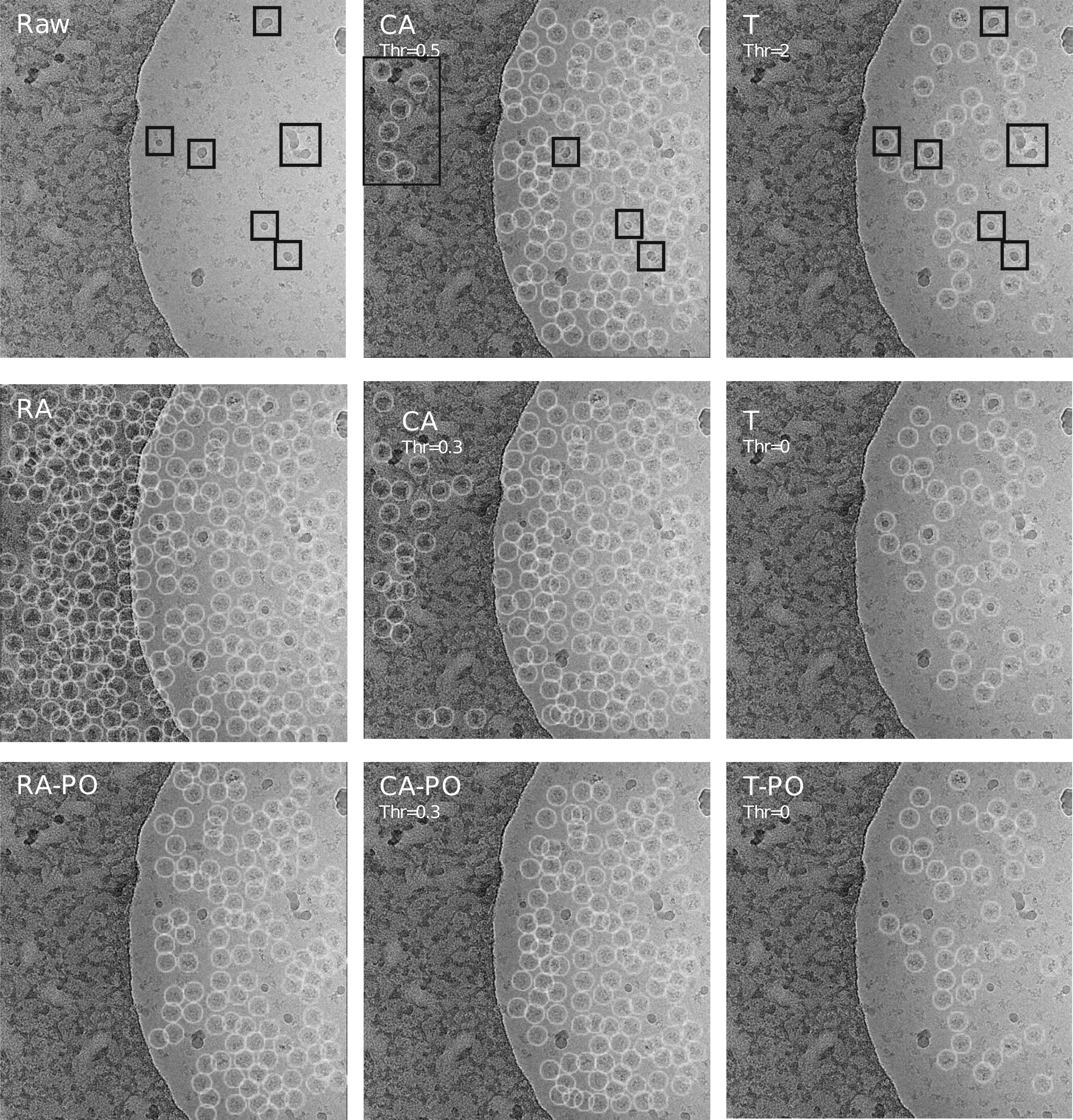
The comparison of PO and applying stricter threshold of particle pickers. The particles selected with RA (R), crYOLO pretrained general model (CA), and Topaz (T) are, respectively, displayed in columns one to three. Top row images correspond to the raw micrograph and the remaining particles after applying a higher threshold to the low threshold crYOLO general and Topaz solutions. The second row images correspond to the low threshold crYOLO general and Topaz solutions and the last row images correspond to the remaining particles after applying PO to the low threshold crYOLO general and Topaz solutions.

However, it comes at the cost of ruling out true-positive particles and many small contaminants are still incorrectly recognized as particles, such as the selections boxed in red. On the contrary, PO removes these false-positive particles more completely, while not affecting the true-positive ones, as shown in the third row of Figure 5; hence, it can be used as a complement for any particle picker independent of threshold decisions.

3.3.2.3. Comparison with the 2D classification

The above experiments have demonstrated that PO is able to reduce the false-positive rates for both conventional and deep learning-based particle pickers. However, it may be argued that such optimization could also be achieved by the subsequent steps in the cryo-EM SPA workflow, particularly at the 2D classification step, which acts as a required step to prune particles. To verify the hypothesis, we compare the particles optimized by PO with the outcome of 2D classification. The RA is chosen to collect the preliminarily picked particles.

Figure 6A shows the class averages calculated from the particles collected by RA. The particles that belonged to “bad classes,” which are marked with a red cross, are ruled out. The remaining particles are shown in Figure 6, where “RA,” “RA & 2D-classes,” and “RA-PO” indicate the particles picked by RA, the particles after conducting a round of 2D classification and discarding the particles belong to “bad classes,” and the particles after the application of PO, respectively. It can be clearly seen that PO is able to remove the particles that lay on the carbon regions and nearby the ice contaminants, while the cleaning of 2D classification still leaves a lot of particles in carbon areas.

FIG. 6.

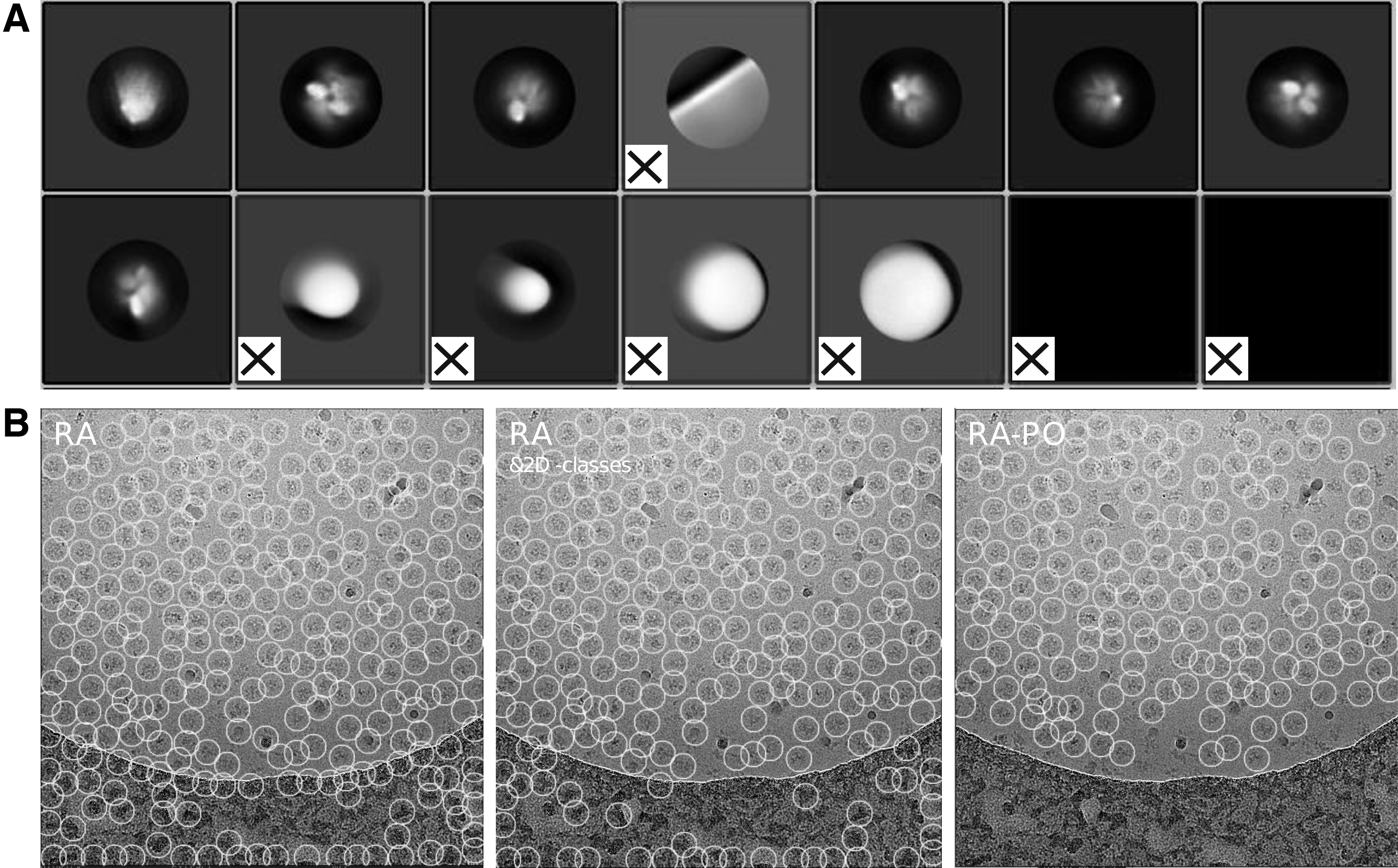
The comparison of 2D classification and PO. (A) The class averages calculated from the particles collected by RA. The class averages marked with a cross are “bad classes” to be dropout. (B) Left to right: (left) particles preminaliarly picked by RA and used as input for 2D-classification; (middle) the remaining particles after cleaning by a round of 2D classification (the particles belongs to “bad” classes are discarded); and (right) the RA-PO. 2D, two dimensional.

3.4. Ablation study

3.4.1. Transfer learning

In this work, we utilize the transfer learning techniques to train the CNN of our approach, where the knowledge gained from public classification datasets is applied to our classification task. As described above, the natural image classification dataset, ImageNet, and the new cryo-EM dataset presented in our work contribute to the pretraining. To verify the performance improvement brought by the transfer learning techniques, we trained three types of models where PO-NoPre means training the neural network from scratch, PO-Pre means fine-tuning the model that is pretrained on ImageNet, and PO means fine-tuning the model that is pretrained on the combination of natural images and cryo-EM images. The macro-F1 score of PO-noPre and PO-Pre is shown in Table 3, and that of PO is shown in Table 2.

Table 3.

The Macro-F1 Scores (%) of PickerOptimizer Variants on Different Datasets

	PO-NoPre			PO-Pre			PO-NoMultiLoss
	10 shots	20 shots	30 shots	10 shots	20 shots	30 shots	10 shots	20 shots	30 shots
10406	55.73	59.98	66.24	83.65	91.57	93.79	91.47	94.91	94.62
10059	57.52	66.77	74.82	87.70	93.92	95.75	97.57	97.97	97.53
10285	65.68	82.01	93.49	92.00	96.45	97.64	97.75	98.85	98.87
10333	73.66	81.47	91.60	91.80	95.91	97.61	97.54	98.81	98.55
10590	81.36	84.61	88.07	94.65	96.58	97.69	98.99	99.30	99.30
10283	62.32	67.71	78.72	89.00	94.29	96.04	96.25	96.97	96.63
10454	38.13	45.81	56.83	52.10	64.59	78.80	75.20	84.10	87.38
10470	33.60	40.75	51.65	51.21	67.20	81.17	78.30	86.05	89.18
10099	80.61	89.67	96.05	88.86	95.25	97.61	96.68	98.26	98.28
10350	69.71	82.76	90.24	89.67	94.17	96.45	95.91	98.17	98.10
10399	92.05	93.85	96.08	91.73	95.24	97.61	96.91	98.21	98.39
10063	84.75	94.14	97.51	92.31	97.70	97.88	97.75	98.69	98.63
10097	76.96	84.11	90.11	82.28	89.56	94.14	94.52	96.54	96.61
10077	54.20	76.47	90.34	91.48	95.51	95.81	95.71	96.74	96.58

Notes: PO-NoPre indicates training the model from scratch, PO-Pre indicates fine-tuning the model that is pretrained on ImageNet, and PO-NoMultiLoss indicates fine-tuning the pretrained model with a single cross-entropy loss. Ten shots, 20 shots, and 30 shots corresponds to 10, 20, and 30 samples in each category of training dataset.

PO, pickerOptimizer.

It can be seen from Table 2 that compared with noPre, which is trained from scratch, the two fine-tuned models show great advantages, achieving an improvement of the macro-F1 score by 20%–30%. This is in line with expectations, since the amount of training data is relatively small, the models of PO-noPre can only learn limited knowledge and easily be overfitted. However, due to the powerful generalization ability obtained from the pretrained model, the PO-Pre and PO are able to achieve the macro-F1 score of more than 90% in most cases.

Furthermore, benefiting from the unique features learned from cryo-EM datasets, the PO model achieved a relatively higher macro-F1 score, above 95% in most cases. Moreover, it is worth noting that the PO model is more robust to the amount of training data, since the impact of different data volumes on the classification performance of the PO model is smaller than the cases of the other two models. The smaller the amount of data, the more obvious the advantages of PO behave.

3.4.2. Multiloss strategy

In this work, we hope to achieve excellent particle optimization performance with minimal user intervention. In other words, we hope to utilize little data to train a classification network with high accuracy, where the problem of overfitting is easy to occur. Therefore, based on an assumption that if the overfitting problem can be suppressed reasonably, the performance of the model will be improved, the multiloss model optimization strategy is proposed in our work.

3.4.2.1. The improvements on classification performance

To verify the effectiveness of this strategy, we designed an ablation experiment in which PO-NoMultiLoss directly uses a single cross-entropy loss as the loss function, and PO uses a combination of multiple cross-entropy losses, as described in the subsubsection 2.1.3. The corresponding macro-F1 scores of classification are shown in Tables 2 and 3. It can be found that the classification metrics of all data sizes (10 shots, 20 shots, and 30 shots) have been improved. It is worth noting that in the case of PO-NoMultiLoss, when the size of training data is 20 shots and 30 shots, the macro-F1 score is almost the same.

Although satisfactory performance has been achieved, it can be found that even if the amount of data is increased from 20 to 30, the classification performance is hardly improved. This is the limitation brought by overfitting, which hinders further improvements in model performance. In contrast to the results of PO-NoMultiLoss, when the amount of data increases, the performance of the PO model is continuously optimized, which means that the overfitting situation is suppressed to a certain extent, and the performance of the model can be further improved.

3.4.2.2. The effects of the weights setting for different loss functions

The weights for different loss functions in multiloss strategy are set as hyperparameters in this work. To find the optimal coefficients, we conducted a series of experiments to test different values. As described in subsubsection 2.1.3, the values of hyperparameters should ensure that the values of different losses are in the same order of magnitude to avoid a situation where one function plays an absolutely dominant role and the others barely play a role.

Based on the experience observed from multiple experiments, we manually set some optional values, and the corresponding results of four public datasets are shown in Table 4. In addition, we tested two different strategies, one using a combination of two cross-entropy loss functions and the other using a combination of three cross-entropy loss functions. In the latter case, the classifier is divided into three branches. Different from the classifier shown in Figure 1C, the feature maps will undergo another branch that contains two continuous 1 × 1 convolutional layers, a GAP pooling, and a fully connected layer. The feature maps will be compressed to 128 dimensions, and then the third loss is calculated.

Table 4.

The Macro-F1 Scores (%) of PickerOptimizer Trained with Different Multiloss Strategies

		10059	10285	10099	10063
Two loss functions	$l_{1} + 0.2 < s u p > * < ∕ s u p > l_{2}$	98.57 ± 0.88	99.19 ± 0.91	98.49 ± 1.31	98.93 ± 0.98
	$l_{1} + 0.3 < s u p > * < ∕ s u p > l_{2}$	98.59 ± 0.94	99.31 ± 0.77	98.57 ± 1.14	98.96 ± 0.93
	$l_{1} + 0.4 < s u p > * < ∕ s u p > l_{2}$	98.52 ± 0.96	99.28 ± 0.97	98.53 ± 1.17	98.85 ± 1.01
Three loss functions	$l_{1} + 0.3 < s u p > * < ∕ s u p > l_{2} + 0.05 < s u p > * < ∕ s u p > l_{3}$	98.48 ± 0.92	99.30 ± 0.74	98.49 ± 1.34	98.90 ± 0.94
	$l_{1} + 0.3 < s u p > * < ∕ s u p > l_{2} + 0.1 < s u p > * < ∕ s u p > l_{3}$	98.57 ± 0.89	99.30 ± 0.81	98.53 ± 1.20	98.91 ± 0.89
	$l_{1} + 0.3 < s u p > * < ∕ s u p > l_{2} + 0.2 < s u p > * < ∕ s u p > l_{3}$	98.51 ± 0.94	99.28 ± 0.83	98.51 ± 1.22	98.91 ± 1.00

Notes: All models are trained with “30 shots.” Boldface indicates the optimal result of the corresponding loss function and dataset.

It can be seen from Table 4 that when using a combination of two loss functions, the best performance is achieved with weights of the two loss functions set to $(1, 0.3)$ . On this basis, continuing to increase the number of loss functions cannot bring a further improvement on the model classification performance. Therefore, in this work, we choose the function of the multiloss strategy as $l o s s = l o s s_{1} + 0.3 * l o s s_{2}$ .

4. CONCLUSIONS

In this work, we introduce a deep learning-based classification model for particle pruning, PO, to separate erroneously picked particles from positive ones. The algorithm is designed to achieve high classification performance with minimal human intervention. Two main techniques are adopted in this work: (1) transfer learning is utilized to leverage the knowledge learned from a large-scale image classification dataset and enable the fine-tuning with minimal data. (2) Multiloss strategy is proposed to alleviate the overfitting problem and further improve the classification performance of the algorithm.

Moreover, to eliminate the huge discrepancy between cryo-EM images and natural images, we constructed the first image classification dataset for cryo-EM, which contains the samples from 14 public datasets. The performance of PO is tested on several public datasets, which demonstrated that PO is a very efficient approach for particle postprocessing, achieving accuracy and F1 scores above 95% in most cases. Moreover, we present three case studies to compare PO with other pruning strategies where the PO achieved better or comparable performance. Therefore, PO is a useful tool to improve conventional particle pickers and complement deep learning-based ones, hence promoting subsequent processing.

AUTHORS' CONTRIBUTIONS

H.L.: conceptualization, methodology, software, formal analysis, investigation, data curation, writing—original draft, and visualization. G.C.: methodology, software, and writing—review and editing. S.G.: writing—review and editing, and validation. J.L.: resources and supervision. X.W.: supervision and funding acquisition. F.Z.: resources, writing—review and editing, supervision, project administration, and funding acquisition.

Footnotes

ACKNOWLEDGMENTS

The authors thank the anonymous reviewers for their helpful comments.

AUTHOR DISCLOSURE STATEMENT

The authors declare they have no conflicting financial interests.

FUNDING INFORMATION

The research is supported by the Strategic Priority Research Program of the Chinese Academy of Sciences (no. XDA16021400), the National Key Research and Development Program of China (nos. 2021YFF0704300, 2017YFA0504702), and the NSFC projects grants (61932018, 62072441 and 62072280).

References

Banerjee

, Bartesaghi

, Merk

, et al. 2016. 2.3 å resolution cryo-em structure of human p97 and mechanism of allosteric inhibition. Science. 351, 871–875.

Bepler

, Morin

, Rapp

, et al. 2019. Positive-unlabeled convolutional neural networks for particle picking in cryo-electron micrographs. Nat. Methods. 16, 1153–1160.

Bottou

2012. Stochastic gradient descent tricks, 421–436. In Neural Networks: Tricks of the Trade. Springer; Berlin, Heidelberg.

Cash

J.N.

, Urata

, Li

, et al. 2019. Cryo–electron microscopy structure and analysis of the p-rex1–g

β γ

signaling scaffold. Sci. Adv. 5: eaax8855.

Deng

, Dong

, Socher

, et al. 2009. Imagenet: A large-scale hierarchical image database. 2009 IEEE conference on computer vision and pattern recognition, IEEE, pp. 248–255.

Fischer

, Neumann

, Bock

L.V.

, et al. 2016. The pathway to gtpase activation of elongation factor selb on the ribosome. Nature. 540, 80–85.

Gao

, Han

, Zeng

, et al. 2021. Macromolecules structural classification with a 3d dilated dense network in cryo-electron tomography. IEEE/ACM Trans. Comput. Biol. Bioinform. 19, 209–219.

Gao

, Cao

, Julius

, et al. 2016. Trpv1 structures in nanodiscs reveal mechanisms of ligand and lipid action. Nature. 534, 347–351.

, Zhang

, Zong

, et al. 2019. Cryo-em structure of the mammalian atp synthase tetramer bound with inhibitory protein if1. Science. 364, 1068–1075.

10.

, Zhang

, Ren

, et al. 2016. Deep residual learning for image recognition. Proceedings of the IEEE conference on computer vision and pattern recognition, pp. 770–778.

11.

Isom

G.L.

, Coudray

, MacRae

M.R.

, et al. 2020. Letb structure reveals a tunnel for lipid transport across the bacterial envelope. Cell. 181, 653–664.

12.

Iudin

, Korir

P.K.

, Salavert-Torres

, et al. 2016. Empiar: A public archive for raw electron microscopy image data. Nat. Methods. 13, 387–388.

13.

Kim

J.H.

, Lee

S.W.

, Kwak

, et al. 2016. Multimodal residual learning for visual qa. NIPS, pp. 361–369.

14.

, Chen

, Gao

, et al. 2021. Pickeroptimizer: A deep learning-based particle optimizer for cryo-electron microscopy particle-picking algorithms. International Symposium on Bioinformatics Research and Applications, Springer, pp. 549–560.

15.

, Zhang

, Wan

, et al. 2022. Noise-transfer2clean: Denoising cryo-em images based on noise modeling and transfer. Bioinformatics. 38, 2022–2029.

16.

Liu

, Zhou

, Zhang

, et al. 2020. Fact caught in the act of manipulating the nucleosome. Nature. 577, 426–431.

17.

Mashtalir

, Suzuki

, Farrell

D.P.

, et al. 2020. A structural model of the endogenous human baf complex informs disease mechanisms. Cell. 183, 802–817.

18.

Nicholson

, Edwards

T.A.

, O'Neill

A.J.

, et al. 2020. Structure of the 70s ribosome from the human pathogen acinetobacter baumannii in complex with clinically relevant antibiotics. Structure. 28, 1087–1100.

19.

Paszke

, Gross

, Massa

, et al. 2019. Pytorch: An imperative style, high-performance deep learning library. NIPS. 32, 8026–8037.

20.

Sanchez-Garcia

, Segura

, Maluenda

, et al. 2018. Deep consensus, a deep learning-based approach for particle pruning in cryo-electron microscopy. IUCrJ, 5, 854–865.

21.

Sanchez-Garcia

, Segura

, Maluenda

, et al. 2020. Micrographcleaner: A python package for cryo-em micrograph cleaning using deep learning. J. Struct. Biol. 210, 107498.

22.

Scheres

S.H.

2012. Relion: Implementation of a bayesian approach to cryo-em structure determination. J. Struct. Biol. 180, 519–530.

23.

Scheres

S.H.

2015. Semi-automated selection of cryo-em particles in relion-1.3. J. Struct. Biol. 189, 114–122.

24.

Schoebel

, Mi

, Stein

, et al. 2017. Cryo-em structure of the protein-conducting erad channel hrd1 in complex with hrd3. Nature. 548, 352–355.

25.

Singh

, Graf

, Linden

, et al. 2020. Discovery of a regulatory subunit of the yeast fatty acid synthase. Cell. 180, 1130–1143.

26.

Song

, Ma

, Gong

, et al. 2017. Crest: Convolutional residual learning for visual tracking. Proceedings of the IEEE international conference on computer vision, pp. 2555–2564.

27.

Tan

Y.Z.

, Baldwin

P.R.

, Davis

J.H.

, et al. 2017. Addressing preferred specimen orientation in single-particle cryo-em through tilting. Nat. Methods. 14, 793–796.

28.

Tan

Y.Z.

, Zhang

, Rodrigues

, et al. 2020. Cryo-em structures and regulation of arabinofuranosyltransferase aftd from mycobacteria. Mol. Cell. 78, 683–699.

29.

Wagner

, Merino

, Stabrin

, et al. 2019. Sphire-cryolo is a fast and accurate fully automated particle picker for cryo-em. Commun. Biol. 2, 1–13.

30.

Wang

, Gong

, Liu

, et al. 2016. Deeppicker: A deep learning approach for fully automated particle picking in cryo-em. J. Struct. Biol. 195, 325–336.

31.

, Zhong

, and Liu

2018. Deep residual learning for image steganalysis. Multimed. Tools. Appl. 77, 10437–10453.

32.

Zhang

, Chen

, Ren

, et al. 2015a. A two-phase improved correlation method for automatic particle selection in cryo-em. IEEE/ACM Trans. Comput. Biol. Bioinform. 14, 316–325.

33.

Zhang

, Zuo

, Chen

, et al. 2017a. Beyond a gaussian denoiser: Residual learning of deep cnn for image denoising. IEEE Trans. Image Process. 26, 3142–3155.

34.

Zhang

, Chen

, Ruan

, et al. 2015b. Cryo-em structure of the activated naip2-nlrc4 inflammasome reveals nucleated polymerization. Science. 350, 404–409.

35.

Zhang

, Sun

, Feng

, et al. 2017b. Cryo-em structure of the activated glp-1 receptor in complex with a g protein. Nature. 546, 248–253.

36.

Zhu

, Carragher

, Glaeser

R.M.

, et al. 2004. Automatic particle selection: Results of a comparative study. J. Struct. Biol. 145, 3–14.