Efficient Colored de Bruijn Graph for Indexing Reads

Abstract

The colored de Bruijn graph is a variation of the de Bruijn graph that has recently been utilized for indexing sequencing reads. Although state-of-the-art methods have achieved small index sizes, they produce many read-incoherent paths that tend to cover the same regions in the source genome sequence. To solve this problem, we propose an accurate coloring method that can reduce the generation of read-incoherent paths by utilizing different colors for a single read depending on the position in the read, which reduces ambiguous coloring in cases where a node has two successors, and both of the successors have the same color. To avoid having to memorize the order of the colors, we utilize a hash function to generate and reproduce the series of colors from the initial color and then apply a Bloom filter for storing the colors to reduce the index size. Experimental results using simulated data and real data demonstrate that our method reduces the occurrence of read-incoherent paths from 149,556 to only 2 and 5596 to 0 respectively. Moreover, the depths of coverage for the reconstructed reads are equal to those for the input reads for the simulated data, whereas the previous method decreases the depth of coverage at many positions in the source genome. Our method achieves quite a high accuracy with a comparable construction time, peak memory size, and index size to the previous method.

1. INTRODUCTION

The de Bruijn graph (dBG) is a data structure that is widely utilized for genome assembly (Pevzner et al., 2001). The colored de Bruijn Graph (cdBG) is a variation of dBG in which each node and edge can store multiple colors. The traditional dBG assumes that all input reads are generated from the same genome, whereas the cdBG can differentiate source genomes and generate contigs associated with different genomes by traversing the nodes storing the same color.

The cdBG was originally introduced for reference-free detection of a genetic variation among a small number of individuals (Iqbal et al., 2012) and has more recently been applied for indexing all the input reads to improve the accuracy of the variation detection (Alipanahi et al., 2018a,b; Díaz-Domínguez, 2019). A similar attempt for disambiguating a large number of paths in the graph has also been examined for a general variation graph constructed from VCF (Pandey et al., 2021).

A modern sequencer produces a huge number of sequencing reads, so reducing the memory consumption for dBG is crucial. Currently, BOSS (Bowe et al., 2012) is widely accepted as a memory-efficient form of dBG, and it is also used as a part of cdBGs (Almodaresi et al., 2019; Almodaresi et al., 2017; Alipanahi et al., 2018a,b; Díaz-Domínguez, 2019; Holley et al., 2015; Muggli et al., 2017).

For example, VARI (Muggli et al., 2017) uses BOSS for a graph and stores the colors of nodes and edges in a binary matrix C, where rows represent k-mers and columns represent colors by using Elias-Fano encoding (Elias, 1974; Fano, 1971; Okanohara and Sadakane, 2007). C is held as a compressed form to reduce memory use. As most other memory-efficient cdBGs take a similar approach to VARI, designing an efficient C is essential, particularly when a cdBG supports read-coherent paths (i.e., when it assigns colors to differentiate each read).

To reduce the size of C, previous studies (Alipanahi et al., 2018b; Díaz-Domínguez, 2019) have reused colors in a greedy manner, and although this is successful in terms of reducing the index size, there is still a problem in that subgraphs causing read- incoherent paths are generated. More precisely, it is not possible to uniquely determine the next node when traversing the subgraphs, which leads to a failure to reproduce some input reads that overlap the subgraphs. We call such an input read an ambiguous sequence.

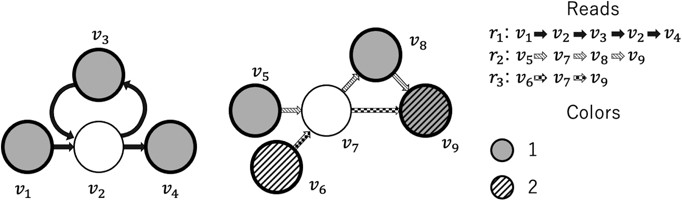
An example is shown in Figure 1, where the subgraphs correspond to three input reads r₁ (embedded as a path: $v_{1} \to v_{2} \to v_{3} \to v_{2} \to v_{4}$ ), r₂ ( $v_{5} \to v_{7} \to v_{8} \to v_{9}$ ), and r₃ ( $v_{6} \to v_{7} \to v_{9}$ ). In the subgraphs, both r₁ and r₂ are assigned the same color 1, and r₃ is assigned color 2. According to the paths that corresponds to r₁, r₂, and r₃, color 1 is recorded at $v_{1}, v_{3}$ , v₄, v₅, and v₈ and color 2 is recorded at v₆ and v₉. We do not have to color all the nodes, and we avoid coloring nodes where the color (or set of colors) can be derived from the previous nodes (e.g., v₂ and v₇).

FIG. 1.

Coloring examples of previous method. Reads r₁ and r₂ cannot be reconstructed because v₂ and v₇ have two successors recording the same color.

We traverse the graph in such a way that we choose nodes that have the same color to find a read-coherent path. Therefore, if we want to find a path that is coherent with a read, we should traverse the nodes that are storing the color of the read. That is, if we encounter a node with more than one successor, the node storing the color of the read should be chosen.

The problem with the coloring scheme of prior works is that it tends to generate subgraphs in which more than one successor have the same color, as illustrated by the subgraphs in Figure 1. For example, the same color is recorded at v₃ and v₄, which are the successors of v₂. v₈ and v₉ are the successors of v₇ and they have the same color. The ambiguity is caused by the underlying structure of the source genome sequence. 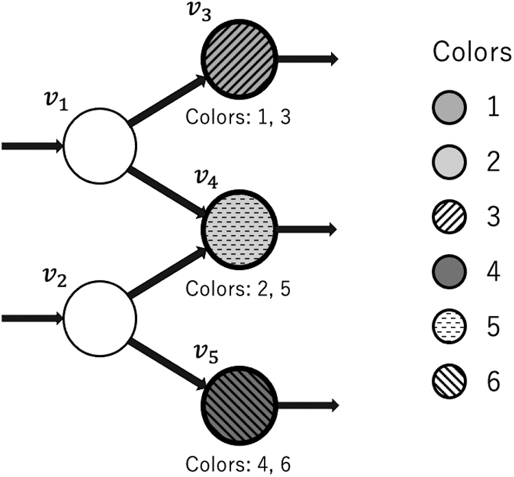In the subgraph on the left, r₁ contains a repeat $(v_{2} \to v_{3} \to v_{2})$ , and in the subgraph on the right, r₂ and r₃ share a substring with a single mutation.

Generally, reads originating from the same region in the source genome overlap the same subgraph, so if a region causes such ambiguity, all the reads covering the region potentially become ambiguous sequences when they are embedded in the cdBG. This means that no read-coherent path can be found by cdBG for such regions. To demonstrate the problem, we show in Figure 2 a case in which all the reads covering a particular region are ambiguous sequences. In fact, we found many such information-lost regions (discussed further in Section 3). Since the regions causing the ambiguity may contain biologically meaningful structural variants, designing a coloring scheme that can avoid producing ambiguous sequences will contribute to the accuracy of the downstream analysis.

FIG. 2.

Example of an information-lost region in the source genome. The horizontal axis shows the position in the source genome and the vertical axis shows the number of reads that support that position. The number of ambiguous sequences increases as it gets closer to the repeat region at the center of the figure, and there are no non-ambiguous sequences in the repeat region.

In this article, we introduce a novel coloring algorithm for cdBG that can index all the input reads accurately. In this algorithm, multiple colors are used for a single read to avoid the ambiguity. Although our approach increases the number of colors, it keeps the index size small by using a hash function-based color generation technique and a Bloom filter. Our experimental results demonstrate that the proposed algorithm reduces the occurrence of ambiguous sequences from 149,556 to only 2 for simulated data and 5596 to 0 for real data while achieving a similar build time, peak memory size, and index size to the previous method.

2. METHOD

In this section, we explain our coloring algorithm in detail. First, we provide definitions and description of related algorithms in Section 2.1. We then explain our concept of coloring based on hash functions in Section 2.2, followed by the detailed construction procedure and the search algorithms in Sections 2.3 and 2.4. Finally, we describe how to compress a color matrix in Section 2.5.

2.1. Preliminaries

2.1.1. Notations

Given a string S, we denote the i-th letter of S by $S [i]$ . The length of S is denoted by $| S |$ . The concatenation of a character c and S is denoted by cS. A substring of S that starts from the i-th letter and ends with the j-th letter is denoted by $S [i . . j]$ . The index starts with 0, that is, $S [0]$ is the first letter of S. For a vector of integer M, we abuse the same notation for a part of M that starts from the i-th element and ends with the j-th element by $M [i . . j]$ . For a binary matrix $C \in {0, 1}^{n \times m}$ , we denote an i-th-row and j-th-column bit by $C [i, j]$ .

2.1.2. Rank and select

Given a string Q of length n that consists of the alphabet $Σ = {1, \dots, σ}$ , a position $i \in {0, \dots, n}$ , and a letter $q \in Σ$ , $r a n k_{q}$ $(Q, i)$ is the number of occurrences of q in $Q [0 . . i - 1]$ and $s e l e c t_{q}$ $(Q, j)$ is the position of the i-th occurrence of q in Q. For example, given a binary string $Q = 001101001$ , $r a n k_{1}$ $(Q, 3) = 1$ and $s e l e c t_{1}$ $(Q, 2) = 3$ . Rank and Select can be computed in constant time by the efficient algorithm (Okanohara and Sadakane, 2007; Raman et al., 2002).

2.1.3. de Bruijn graph

A dBG is a labeled directed graph 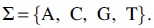$G = (V, E)$ , where V is a set of nodes and E is a set of edges. A node $v \in V$ is labeled with a $(k - 1)$ -mer appearing in a set of strings R. For two nodes $v_{i}, v_{j} \in V$ , v_i has a directed edge $e_{i j} \in E$ toward v_j if the $k - 2$ suffix of v_i's label matches the $k - 2$ prefix of v_j's label and if R contains a k-mer whose $k - 1$ prefix and $k - 1$ suffix match v_i's label and v_j's label, respectively. A read r is a string consisting of an alphabet . In this study, R consists of a set of reads ${r_{1}, r_{2}, \dots, r_{n}}$ and its reverse complements ${r_{1}^{r c}, r_{2}^{r c}, \dots, r_{n}^{r c}}$ .

In principle, our algorithm can use any form of dBG as long as any node in dBG is uniquely identified. We use BOSS (Bowe et al., 2012) in this study to take advantage of its memory efficiency. BOSS (Bowe et al., 2012) is a succinct representation of dBG and is based on an idea similar to BWT (Burrows and Wheeler, 1994). It performs various graph operations within an efficient computation time (e.g., the numbers of outgoing and incoming edges of a node can be computed in constant time) while consuming only a small amount of memory. BOSS supports the following operations.

$o u t d e g r e e$ $(G, v)$ : return the number of outgoing edges of v.

$o u t g o i n g$ $(G, v, t)$ : return the id of v's successor that links to v by the edge labeled with t.

$i n d e g r e e$ $(G, v)$ : return the number of incoming edges of v.

$i n c o m i n g$ $(G, v, t)$ : return the id of v's predecessor that links to v by the edge labeled with t.

$n o d e$ _ $t o$ _ $l a b e l$ $(G, v)$ : return the label of node v.

In addition to the above, our algorithm implements the following operations that are used in the previous research (Díaz-Domínguez, 2019). These operations can also be computed efficiently.

$o u t g o i n g$ _ $r$ $(G, v, i)$ : return the id of v's successor that is connected from v by the i-th outgoing edge in lexicographical order.

$i n c o m i n g$ _ $r$ $(G, v, i)$ : return the id of v's predecessor that is connected to v by the i-th incoming edge in lexicographical order.

$l a b e l$ _ $t o$ _ $n o d e$ $(G, S)$ : return the id of the node labeled with S.

$g e t$ _ $e d g e$ _ $s y m b o l$ $(G, v, i)$ : return the symbol of the i-th outgoing edge of $v .$

2.1.4. Colored de Bruijn graph

A cdBG is an extension of the dBG. It records a set of colors at each node (or edge). The color c is added to a node v if the input read r is assigned the color c and the label of v is a $k - 1$ substring of r. The colors are maintained in a binary matrix $C \in {0, 1}^{n \times m}$ , where n is the number of nodes and m is the number of colors. If the color c_j is contained in the color set of node v_i, we denote $C [i, j] = 1$ , and $C [i, j] = 0$ otherwise.

To reduce the number of columns in C, we categorize a node into four types—start, end, critical, and non-colored—and give colors only to the start, end, and critical nodes because the color of a non-colored node can be derived from its predecessor node, which is the same technique used in the previous study (Díaz-Domínguez, 2019). The start node is the node that represents the beginning of a read r.

The label of the node is $ $r [0 . . k - 3]$ , where $ is the terminal symbol that precedes the other symbols in $Σ$ in lexicographical order. Similarly, the end node is the node that represents the tail of r. The label of the node is $r [n - k + 3 . . n - 1]$ $, where n is the length of r. The critical node is a node that is neither the start nor end node, and whose predecessor node has at least two outgoing edges.

Our algorithm needs the following operations on dBG and C. We will show how to implement them in Sections 2.3 and 2.5.

$i s$ _ $c o n t a i n e d$ $(G, C, v, c)$ : return $t r u e$ if a color c is recorded in v, otherwise $f a l s e$ .

$g e t$ _ $c o l o r$ _ $n u m$ $(G, C, v)$ : return the number of colors recorded in v.

2.2. Concept of proposed coloring scheme

As described in Section 1, the previous approach generates ambiguous subgraphs in which a node has several successors storing the same color. A simple way to solve this problem is to use different colors for a single read depending on the position in the read, so that we can choose a correct node. Consider the case where a read is CATATC and k = 3, and the topology is that of the left graph in Figure 1. v₁, $v_{2},$ v₃, and v₄ are labeled with CA, AT, TA, and TC, respectively.

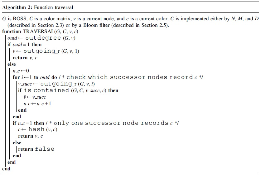
If we assign the i-th 2-mer a color i (e.g., CA is assigned 0 and AT is assigned 1), the colors of v₁, v₂, v₃, and v₄ become 0, {1, 3}, 2, and 4. Starting from v₁, we can traverse $v_{1} \to v_{2} \to v_{3} \to v_{2} \to v_{4}$ , as we know a color is increasing from the left end toward the right end of the read. The naïve method to achieve this is to create an additional index that memorizes the order of the colors for all the reads; however, this requires a huge amount of memory.

To maintain the order of the colors without using an additional index, we utilize a hash function to generate a series of colors such that the color of the node to be visited next can be reproduced from the color of the current node.

To introduce the key idea, we use a toy example shown in Figure 3. In our algorithm, we assume the topology of the graph and the type of each node are given before assigning colors. For the toy example, we assign color 1 to read r₁. The series of colors used for embedding r₁ is determined by a hash function in such a way that a next color is computed by a current node ID and a current color. In the first step, we record 1 at v₁ because r₁ starts at v₁ and the color of r₁ is 1. In the second step, we compute a new color $c' =$ hash $(v_{1}, 1)$ .

FIG. 3.

Example of coloring by our method for the same graph as Figure 1. Start nodes v₁, v₅, and v₆, end nodes v₄ and v₉, and critical nodes v₃ and v₈ need to be colored. To embed r₁ on the graph, we visit $v_{1} \to v_{2} \to v_{3} \to v_{2} \to v_{4}$ and assign colors. The initial color 1 is assigned to v₁ and the new color $h a s h (v_{1}, 1)$ is generated. We do not assign the color at v₂ and we store $h a s h (v_{1}, 1)$ at v₃ and generate the new color $h a s h (v_{3}, h a s h (v_{1}, 1))$ when we visit v₃. We do not assign the color when we visit v₂ and store $h a s h (v_{3}, h a s h (v_{1}, 1))$ when we visit v₄. r₁ is reproduced in the same manner as it was embedded. The initial color is obtained at v₁ and the next color is computed by $h a s h (v_{1}, 1)$ . When we visit v₂, v₃ is chosen because v₃ has $h a s h (v_{1}, 1)$ . Then we compute $h a s h (v_{3}, h a s h (v_{1}, 1))$ . After visiting v₂, we choose v₄ because v₄ has $h a s h (v_{3}, h a s h (v_{1}, 1))$ . r₂ and r₃ are embedded and reproduced in the same manner. Note that v₈ has $h a s h (v_{5}, 1)$ and v₉ has $h a s h (v_{6}, 2)$ and $h a s h (v_{8}, h a s h (v_{5}, 1))$ and we can correctly embed r₂ and r₃.

As mentioned in the previous section, we do not color all the nodes but only the start, critical, and end nodes. Therefore, we do not color v₂ and we store a color $c'$ at v₃ (a critical node after visiting v₂). In the third step, we compute a new color $c'' =$ hash $(v_{3}, c')$ . $c''$ is recorded at the end node v₄ after visiting v₂.

2.3. Construction of a color matrix

Our method begins by constructing a BOSS G of an input read set R and scanning G to determine the type of each node. It then traverses on G for all the reads and counts how many times each node is visited if the node is either a start, end, or critical node. We denote the number of colored nodes by p and a count for the i-th colored node by $δ_{i}$ . After the above prepossessing step, we construct a color matrix C by Algorithm 1.

As described in Section 2.1, C is an $n \times m$ bit matrix that shows the existence of each color for each node. For memory efficiency, we use $N \in {0, 1}^{n}$ , $D \in {0, 1}^{ℓ}$ , and $M \in Z_{\geq 0}^{ℓ}$ to replace C, where n is the number of all nodes in a graph G, and $ℓ = \sum_{i = 0}^{p - 1} δ_{i}$ . Each bit in N shows whether or not the corresponding node has a color. When a node v has a color, $N [v] = 1$ , and $N [v] = 0$ otherwise. By using N, we can compute the order of the colored node by $r a n k_{1} (N, v),$ given a node v. M stores colors assigned to each node in such a way that a vector of colors stored in each colored node is concatenated.

To identify the set of colors of an i-th colored node, we use D, which is a concatenation of $δ_{i}$ bits, where the first bit is 1 and the other $δ_{i} - 1$ bits are 0s (e.g., $D = 10 \dots 010 \dots$ ). By computing $s e l e c t_{1} (D, i + 1)$ , we can identify the positions in M where colors of the i-th colored node are stored. Before running Algorithm 1, M is initialized such that all the elements are 0s.

In our coloring method, a series of colors for embedding a read is added read by read. In Line 3 of Algorithm 1, a terminal symbol $ is added at the head and tail of a read r so that we can distinguish the beginning and end of the read. In Line 4, the start node v for r is obtained and we compute the order of v within the colored nodes in Line 5. In Line 6, a set of colors T already assigned to v is obtained, and we compute $c = m i n {c | c \in Z_{\geq 0} ∖ T}$ as the initial color for r.

In Line 7, the position of the first 0 (i.e., the first position of empty elements) within the range is obtained by a binary search and c is stored at the position in Line 8. In Line 9, the next color to be used is computed by hash $(v, c)$ . The rest of the nodes that are visited for embedding r are colored in the same way. In Lines 10–18, we compute the next node, and if the type of the node is either critical or end, we add the color to the node and compute the next color. After running Algorithm 1, the functions get_color_num $(G, C, v)$ and is_contained $(G, C, v, c)$ are computed by counting the number of non-zero values and checking the membership of c in .

2.4. Search on the color matrix

Once we construct a color matrix C, we can easily find a read-coherent path. Algorithm 2 describes a traverse. Given G, C, a node v, and a color c, it returns the next node and color. Note that it returns false when the next color is contained in more than one successor of v, as we cannot uniquely determine the next node. Such a case could happen due to a hash collision. For example, as shown in Figure 4, if two reads r₁ and r₂ share a path $v_{1} \to v_{2}$ and the hash values based on the initial colors of r₁ and r₂ happen to become the same, the v₃ that should be visited for r₁ and the v₄ that should be visited for r₂ have the same color, since we do not check such a collision in Algorithm 1.

FIG. 4.

Examples of ambiguous sequences in our method. The upper graph shows an example where the same hash value is generated at the same node v₁ for reads r₁ and r₂, and the same color is recorded at each successor node, resulting in ambiguity. The lower graph shows an example where the same hash value is generated at v₅ and v₈ and stored at v₇ and $v_{10}$ for reads r₃ and r₅, respectively, which causes the ambiguity that v₆ has two successors containing the same color.

The other example with r₃, r₄, and r₅ is caused by a similar reason. Although such a collision generates ambiguous sequences, we should emphasize that a hash collision happens randomly, so the probability of such an ambiguity occurring at the same node is quite small. This means that, since an ambiguous read covers a random position in the source genome, we can maintain the depth of read coverage for any position in the source genome—unlike the previous method, which tends to lose all the read-coherent paths for a particular region. The occurrence of a hash collision can be mitigated if we use a hash function that maps to a large space; however, this causes an increase in the size of M.

2.5. Compressing the color matrix by Bloom filter

In the previous section, we explained the color matrix consisting of N, D, and M. Since our algorithm needs several colors to embed each read, M becomes large, particularly when the colors are randomly distributed over a large space. In our implementation, we used 64 bits for each color to avoid a hash collision. After constructing the color matrix, M is utilized to check whether a given color is contained in a given node, and we do not have to hold all the colors explicitly. In this subsection, we propose a space efficient method to enable the membership query while achieving a small false positive rate.

The key detail of the membership query in our case is that we know all the potential queries for a given node v, since we already know the topology of the graph and the set of colors stored in each node. That is, when we visit a node with multiple outgoing edges, the color that is used for selecting the next node is always stored in one of the successors, as per the definition of our coloring scheme. Let us define a set $α$ as all colors recorded in v and a set $β$ as all colors recorded in all the successors of v's predecessors except for v. The goal is to check whether a color $c \in α \cup β$ holds $c \in α$ . An example of $α$ and $β$ is shown in Figure 5.

FIG. 5.

Example of $α$ and $β$ . For the membership query for node v₄, $α$ is the set of colors stored at v₄, that is, $α = {2, 5}$ , and $β$ is the colors stored at v₃ and v₅, that is, $β = {1, 3, 4, 6}$ .

We use a Bloom filter (Bloom, 1970) for the membership query (see Section 1 of the Supplementary Material S1 for a brief explanation of the Bloom filter). To reduce the filter size, we examine the length of a bit vector and the number of hash functions from a small value toward a large value until the ones that achieve a false positive rate $\leq p$ are found. The filter for v is built as follows, where s is a length of a bit vector. To achieve smaller s while satisfying a given false positive rate p, using smaller ds is ideal; however, the smaller ds increases construction time.

(1)

Scan cdBG and obtain $α$ and $β$ for v, and initialize s with s₀.

(2)

Determine the number of hash functions as $⌈ (s ∕ | α |) \times 0.7 ⌉$ .

(3)

Add all the colors in $α$ to the filter.

(4)

Check membership of all the colors in $β$ and compute the false positive rate.

(5)

Build the filter if the false positive rate is less than or equal to p; otherwise, set $s = s + d s$ , where ds is an increase of s, and return to step 2.

Note that this simple method can achieve a smaller filter size compared to the approach based on minimal perfect hash function. We find $α$ and $β$ by traversing the predecessors and their successors in a straightforward manner. The pseudo-code including the traverse is shown in Algorithm 1 in the Supplementary Material S1. In our analysis, the average bit length for storing a single color is 1.61–3.49 for our method (when $p = 0.00001$ ), while the bit length estimated based on the information theoretically lower bound is 4.88 for the minimal perfect hash-based approach.

See Section 2 of the Supplementary Material S1 for a more detailed discussion. Note that the bit lengths are slightly different from the values presented in Section 3, since we need to assume the case where nodes with $| β_{i} | = 0$ are excluded for fair comparison. The Bloom filters (i.e., bit vectors) of colored nodes are concatenated into a single bit vector B and the positions of each filter are recorded by another bit vector K. K is a concatenation of bits of an equal length to each filter in which the first bit is 1 and rest are 0s.

In the compressed form of C, the function is_contained $(G, C, v, c)$ is computed using the Bloom filter. Given a node v, the Bloom filter f of v is extracted by N, D, K, and B. The number of hash functions used for a filter can be computed by $⌈ (x ∕ y) \times 0.7 ⌉$ , where x is the filter length, which can be computed from N, D, and K, and y is the number of colors stored in v, which can be computed from N and D.

In our method, the i-th hash function is implemented by $(h a s h_{1} (c) + i \times h a s h_{2} (c))$ , where $h a s h_{1}$ and $h a s h_{2}$ are pseudo-random hash functions (as introduced in a study showing that the implementation does not increase asymptotic false positive probability [Kirsch and Mitzenmacher, 2006]). After computing B and K, we can discard M.

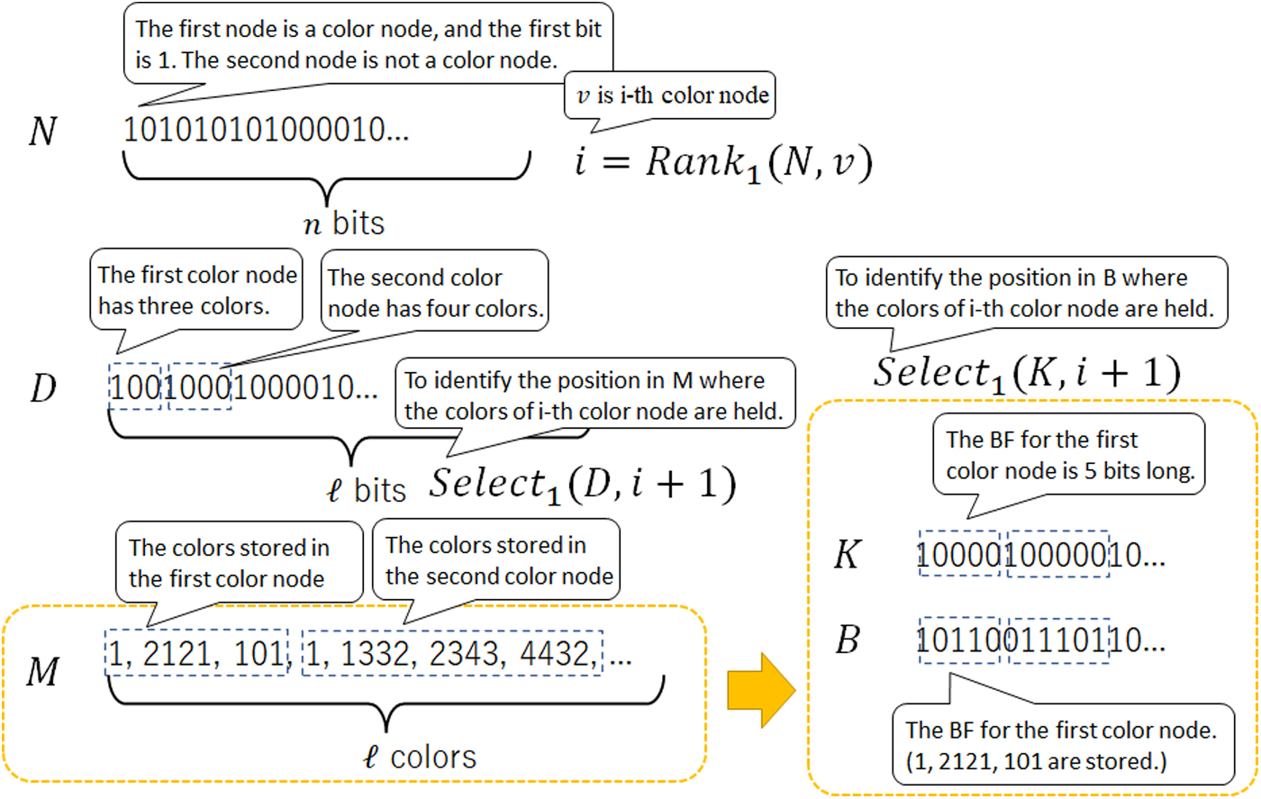
Figure 6 shows the summary of the color matrix. As shown in the figure, the position in B for the filter of i-th color node is extracted by $s e l e c t_{1} (K, i + 1)$ and we can check if a given color is stored in i-th node. Each Bloom filter is built in a way that we try with a short filter firstly and increases the length of the filter by ds bits until the false positive rate becomes smaller than the given threshold p. We will show the trade-off between the size of B and building time of B in Section 3.

FIG. 6.

The summary of the color matrix. After obtaining the node id v from dBG, the colors stored in v are computed using N, D, and M. M, which directly holds colors, is replaced by the Bloom filters B, which is more space-efficient. The filter for each color node is extracted by K.

Given a start node v and an initial color c₀, we can find a read-coherent path by running Algorithm 2. Although c₀ is not explicitly given, it can be found by using v's filter. In our construction algorithm, the initial color assigned to each read is the minimum number except for the colors already stored. The colors assigned to critical and end nodes are generated by a hash function. Since the hash function maps to a large space, the initial color (i.e., the color assigned to a start node) is usually 1.

Therefore, we know the initial color by checking the membership of 1 in v's filter. If v is a start node of multiple reads, the initial colors for the reads become $1, \dots, n$ , where n is the number of reads. The potential drawback of this compression is that we need to search a start node if we begin a traversal from a non-start node; however, we consider the additional time to reach a start node is negligible if the depth of coverage for the input reads is sufficiently large. Recording the colors without using the Bloom filter on some nodes mitigates this drawback, but increases the index size.

3. EVALUATION

We implemented our algorithm and compared it with a state-of-the-art method (Díaz-Domínguez, 2019) to evaluate the performance. Since a suffix tree (Sadakane, 2007) is often used for indexing genome sequences and we can perform the necessary operations for finding a read-coherent path, we also compared our algorithm with the suffix tree. Note that using only FM-Index for finding a read-coherent path is quite time consuming, so we did not make a comparison with FM-Index.

3.1. Data sets and implementation

We tested our method both on simulated data and real data. The simulated read sets were generated from chromosome 21 of the human reference genome (GRCh38) using Art (Huang et al., 2012). We utilized the HiSeq2000 error profile and generated 100 bp single-end reads. The number of reads was $14, 044, 878$ , the average depth of coverage was 40 × , and the error rate was $0.75 %$ . We did not use a simulated read if it included N.

Since our algorithm indexes the reverse complements of the input reads, $28, 089, 756$ strings were indexed in total. We call this data Simdat 1. To evaluate our algorithm on error-corrected reads, we also created a read set in which reads are copied from the same start positions and the same strands in the reference genome without generating sequencing errors. We call this data Simdat 2.

For the real read sets, we downloaded the whole genome sequencing data of Escherichia coli (ERR4785033) from NCBI Sequence Read Archive (https://www.ncbi.nlm.nih.gov/sra) and excluded reads including N. We call this data Realdat 1. The number of reads for Realdat 1 was $3, 042, 154$ , and the average depth of coverage was 90 × . $6, 084, 308$ strings were indexed in total. We also created error-corrected reads from Realdat 1 by using BFC (Li, 2015) with default parameters and call this data Realdat 2. The number of reads for Realdat 2 was $3, 056, 624$ , and the average depth of coverage was 90 × . $6, 113, 248$ strings were indexed in total.

We implemented our algorithm and the suffix tree by using SDSL-lite library (Gog, 2013). The hash function is implemented similarly to the one in Boost (Boost.org, 1999) that is based on the computationally efficient algorithm (Wheeler and Needham, 1994) (see Listing 1 in the Supplementary Material S1). All the programs were compiled with the -O3 optimization option and run on a machine equipped with Intel(R) Core(TM) i7-7820X CPU@3.60GHz and 125GB of RAM.

For each method, we built indices and measured the execution time, peak memory, and index size. Since our method and the previous method support multiple threads for building an index, we used 16 threads. The dBG was constructed with 30-mer for both methods, and the suffix tree was built by a single thread. For our method, we tested three different parameter settings: #1 $d s = | α |$ , #2 $d s = 1$ if $| β | < 2 | α |$ and $s < 2 | α |$ , and $d s = | α |$ otherwise, and #3 $d s = 1$ . Note that ds is the increase in the length of a Bloom filter when finding a filter that satisfies a given false positive rate. Therefore, smaller ds enables a smaller index size, though smaller ds requires a long building time. Our implementation is available at: https://github.com/cBioLab/hash_cdbg.

3.2. Results on simulated data

The results of the index construction are shown in Table 1, where we can see that our method achieved an index building time, peak memory, and index size comparable to those of the previous method. There was a trade-off between the index building time and the index size depending on the setting of ds in our method.

Table 1.
Results of Index Construction for the Simulated Read Sets

Data Method Building time of entire index (hh:mm:ss) Building time of C (hh:mm:ss) Peak memory (GB) Entire index size (MB) Size of C (MB)

Simdat 1 Suffix tree 00:22:14 — 23.8 5649 —

Previous 01:31:07 00:42:13 29.8 986 451

Ours #1 01:27:52 00:38:58 35.4 1028 493

Ours #2 02:12:32 01:23:38 30.2 875 340

Ours #3 13:23:42 12:34:48 35.4 835 300

Simdat 2 Suffix tree 00:21:42 — 23.8 5748 —

Previous 01:24:07 00:40:32 25.8 707 418

Ours #1 01:14:23 00:30:47 27.6 761 473

Ours #2 02:33:05 1:49:30 31.6 603 315

Ours #3 30:14:57 30:14:57 27.6 554 266

Data	Method	Building time of entire index (hh:mm:ss)	Building time of C (hh:mm:ss)	Peak memory (GB)	Entire index size (MB)	Size of C (MB)
Simdat 1	Suffix tree	00:22:14	—	23.8	5649	—
Previous	01:31:07	00:42:13	29.8	986	451
Ours #1	01:27:52	00:38:58	35.4	1028	493
Ours #2	02:12:32	01:23:38	30.2	875	340
Ours #3	13:23:42	12:34:48	35.4	835	300
Simdat 2	Suffix tree	00:21:42	—	23.8	5748	—
Previous	01:24:07	00:40:32	25.8	707	418
Ours #1	01:14:23	00:30:47	27.6	761	473
Ours #2	02:33:05	1:49:30	31.6	603	315
Ours #3	30:14:57	30:14:57	27.6	554	266

We examined three different parameter settings: #1, #2, and #3. The building time of entire index includes that of C, and the entire index size also includes the size of C

When we used settings #2 or #3, our method achieved the smallest index size. The suffix array generated an index more than five times larger than our method and the previous method, though its index building time was small. When we counted the number of colors (i.e., $ℓ$ ) and computed the average bit length per color used in the Bloom filter, we found that #3 achieved 1.58 for Simdat 1 and 1.52 for Simdat 2. As for a compiler option, we found that the -O3 optimization affected the peak memory. When we compiled without the optimization option, all the peak memory became $30.2$ GB for Simdat 1 and $27.6$ GB for Simdat 2.

To evaluate the efficiency of the constructed indices, we reconstructed all the input reads and their reverse complements (i.e., $28, 089, 756$ reads) from the indices. (See Algorithm 2 in the Supplementary Material S1 for the entire algorithm used to reconstruct a read.) As shown in Table 2, our method generated at most 10 ambiguous sequences, whereas the previous method generated $149, 556$ and $182, 434$ ambiguous sequences for Simdat 1 and Simdat 2.

Table 2.

Results of Reconstructing Original Reads from the Indices for the Simulated Read Sets

Data	Method	Reconstruction time (hh:mm:ss)	Peak memory (GB)	Ambiguous sequences
Simdat 1	Suffix tree	00:12:56	12.39	0
	Previous	03:54:43	5.03	149,556
	Ours #1	00:50:39	5.68	2
	Ours #2	00:50:26	5.53	2
	Ours #3	00:50:26	5.49	2
Simdat 2	Suffix tree	00:12:54	12.48	0
	Previous	05:02:38	4.71	182,434
	Ours #1	00:35:14	5.31	7
	Ours #2	00:35:06	5.15	6
	Ours #3	00:35:02	5.11	10

The peak memories are generally proportional to the index size, but the reconstruction time differs significantly between the previous method and ours. Since we set the false positive probability $p = 0.00001$ when building the filter, our method was able to greatly reduce the number of ambiguous sequences.

The peak memories of our method and the previous method are comparable, and that of the suffix tree was twice as large as our method and the previous method. The reconstruction time of our method was significantly faster compared to the previous method. In the previous method, the membership query is conducted in such a way that all the colors in a node v are reconstructed and then scanned, which requires a time linear to the total number of colors stored in nodes to be visited.

In contrast, our method conducts the membership query more efficiently by using a Bloom filter, which only requires a time linear to the number of hash functions. We note that other state-of-the-art cdBGs (Almodaresi et al., 2017; Muggli et al., 2017) also require the constant number of rank/select operations on the compressed data structures for finding a color in a node. The time difference between our method and the Suffix tree can be interpreted as the overhead of finding colors.

We examined three different settings for Bloom filters, that is, three different $d s .$ ds is a parameter for the trade-off between the filter length and the building time. The number of hash functions used for each filter is determined by $⌈ (s ∕ | α |) \times 0.7 ⌉$ , which was almost the same for different ds. Therefore, the membership query times were almost same for the three settings. (Note that s does not so largely differ unless we use very large ds.) Since the number of colors increases as the input read set becomes larger, we consider that our method, which scales to a large dataset, is useful in practice.

We also computed the depth of the coverage for the reconstructed reads at all the positions in chromosome 21 of the human reference genome except for N ( $35, 106, 642$ bases, in total) to evaluate the amount of information-lost regions. Table 3 shows the number of bases (positions) whose depths were 0, $\leq 5$ , or $\leq 10$ . For comparison, we also computed the depth of the coverage for the input reads. As is clear from the results, the depth for the reconstructed reads by our method is the same as that for the input reads, whereas that by the previous method is shallow for many positions, potentially causing a deterioration of the quality of downstream analysis.

Table 3.

Results of Number of Bases in Chromosome 21 of the Human Reference Genome Except for N ( $35, 106, 642$ Bases, in Total) That Had Depths of 0, 5 or Less, or 10 or Less by the Reconstructed Reads

Data	Method	Depth = 0	Depth ≤5	Depth ≤10
Simdat 1	Input	37	371	734
	Previous	2024	19,418	51,887
	Ours #1	37	371	734
	Ours #2	37	371	734
	Ours #3	37	371	734
Simdat 2	Input	37	371	734
	Previous	24,207	53,072	104,213
	Ours #1	37	371	734
	Ours #2	37	371	734
	Ours #3	37	371	734

With our method, the results were the same as the original read sets used as input to create indices, but with the previous method, the depth became shallow for many bases.

3.3. Results on real data

We also conducted the experiments using real read sets. Table 4 shows the results of the index construction. Overall, the results show a similar tendency that was observed in the results of the simulated data, except that the results of our methods based on #2 setting ( $d s = 1$ if $| β | < 2 | α |$ and $s < 2 | α |$ , and $d s = | α |$ otherwise) and #3 setting ( $d s = 1$ ) are similar, where ds is an increase of the size of Bloom filter.

Table 4.
Results of Index Construction for the Real Read Sets

Data Method Building time of entire index (hh:mm:ss) Building time of C (hh:mm:ss) Peak memory (GB) Entire index size (MB) Size of C (MB)

Realdat 1 Suffix tree 00:08:44 — 4.31 1974 —

Previous 00:24:45 00:13:42 2.89 227 119

Ours #1 00:20:15 00:09:12 6.39 259 150

Ours #2 00:27:00 00:15:57 6.22 183 74

Ours #3 00:26:38 00:15:35 6.21 179 70

Realdat 2 Suffix tree 00:04:21 — 3.12 1450 —

Previous 00:22:57 00:12:40 2.50 178 108

Ours #1 00:18:20 00:08:03 5.71 211 141

Ours #2 00:25:06 00:14:49 5.53 136 66

Ours #3 00:25:38 00:15:21 5.52 132 62

Data	Method	Building time of entire index (hh:mm:ss)	Building time of C (hh:mm:ss)	Peak memory (GB)	Entire index size (MB)	Size of C (MB)
Realdat 1	Suffix tree	00:08:44	—	4.31	1974	—
Previous	00:24:45	00:13:42	2.89	227	119
Ours #1	00:20:15	00:09:12	6.39	259	150
Ours #2	00:27:00	00:15:57	6.22	183	74
Ours #3	00:26:38	00:15:35	6.21	179	70
Realdat 2	Suffix tree	00:04:21	—	3.12	1450	—
Previous	00:22:57	00:12:40	2.50	178	108
Ours #1	00:18:20	00:08:03	5.71	211	141
Ours #2	00:25:06	00:14:49	5.53	136	66
Ours #3	00:25:38	00:15:21	5.52	132	62

We examined three different parameter settings: #1, #2, and #3. The building time of entire index includes that of C, and the entire index size also includes the size of C.

For the case using #3 setting, the filter construction cost becomes high for a node storing a large number of colors that has siblings storing many colors, which could be a computational bottleneck, especially when the number of colors stored in siblings is large (i.e., $| α |$ is large and $| β |$ is larger than $| α |$ ). The cdBG of the simulated read sets, which is originated from a human genome, includes a higher ratio of such nodes compared to the real read sets, which is originated from E. coli. For example, a node with more than 10 colors having siblings with more than twice as many colors as the node has (i.e., $| α | > 10$ and $| β | > 2 | α |$ ) was 0.03% of all the nodes for Realdat 1, and 0.22% of all the nodes for the Simdat 1.

Our method achieved the smallest index size, while the peak memory size of the previous method was the smallest. Realdat 2 is an error-corrected read set, which includes a slightly smaller number of reads and is expected to include a smaller number of errors that may cause an increase in the number of nodes and colors. The results also show that the building time, the peak memory size, and the index size of Realdat 2 are smaller than those of Realdat 1 for all the methods.

We also reconstructed all the input reads and their reverse complements and summarized the results in Table 5. Our methods generated no ambiguous sequences, whereas the previous method generated several thousand ones. Note that we cannot evaluate the depth of coverage for each position in the reference genome because we cannot know the true positions where each read was sequenced.

Table 5.

Results of Reconstructing Original Reads from the Indices for the Real Read Sets

Data	Method	Reconstruction time (hh:mm:ss)	Peak memory (GB)	Ambiguous sequences
Realdat 1	Suffix tree	00:02:07	3.87	0
	Previous	00:49:00	1.97	5596
	Ours #1	00:13:42	1.97	0
	Ours #2	00:13:39	1.89	0
	Ours #3	00:13:38	1.89	0
Realdat 2	Suffix tree	00:01:25	3.10	0
	Previous	00:50:48	1.92	6484
	Ours #1	00:11:13	1.96	0
	Ours #2	00:11:10	2.02	0
	Ours #3	00:11:09	1.84	0

4. CONCLUSION

In this work, we developed a new method for indexing sequencing reads by a cdBG. The proposed method uses different colors for a single read depending on the position in the read to reduce the generation of ambiguous subgraphs such as two successor nodes having the same color. To avoid having to memorize the order of the colors, we utilized a hash function to generate colors so that the series of colors can be reproduced from the initial color.

We also proposed using a Bloom filter for holding a set of colors at a node to reduce the index size. We implemented our method and compared it with the previous method and a suffix tree by using simulated data and real data. The results showed that our method significantly reduced the generation of ambiguous subgraphs, and the number of input reads that could not be reconstructed was at most only 10 for simulated data and 0 for real data, whereas the previous method could not reconstruct at least 149,556 reads for simulated data and 5596 reads for real data.

We also confirmed that the depths of coverage for the reconstructed reads were equal to those for the input reads when using our method, whereas the previous method decreased the depth of coverage at many positions in the source genome. Our method achieved such a high accuracy with a comparable construction time, peak memory size, and index size to the previous method, and the index size was one-fifth that of the suffix array. In addition, the membership check of a color in our method requires only a time linear to the number of hash functions used in a Bloom filter and does not depend on the bit length of colors stored in a node.

One of the future works is to extend the method to a dynamic cdBG, considering the growing interest in an updatable data structure (Holley and Melsted, 2020; Muggli et al., 2019). The potential approach is to use a dynamic dBG (Alipanahi et al., 2021) instead of BOSS, which still enables a correct graph traversal after deleting a node; however, after adding a node, it is necessary to change the colors of nodes around the node, which may require a high computational cost. Although some challenges remain, our findings demonstrate the efficiency of our method, and we believe it will contribute to the analysis of large-scale sequencing data.

Footnotes

ACKNOWLEDGMENT

The authors thank Mr. Taiki Yamada for fruitful discussions.

AUTHORs' CONTRIBUTIONS

N.H.: conceptualization, methodology, software, writing—original draft. K.S.: conceptualization, methodology, writing—review and editing, supervision.

AUTHOR DISCLOSURE STATEMENT

The authors declare they have no conflicting financial interests.

FUNDING INFORMATION

The part of the research is supported by Kayamori Foundation of Informational Science Advancement.

SUPPLEMENTARY MATERIAL

References

Alipanahi

, Kuhnle

, Boucher

Recoloring the colored de bruijn graph. In: International Symposium on String Processing and Information Retrieval; pp. 1–11. Springer; 2018b.

Alipanahi

, Kuhnle

, Puglisi

, et al. Succinct dynamic de bruijn graphs. Bioinformatics, 2021; 37(14):1946–1952.

Alipanahi

, Muggli

, Jundi

, et al. Resistome snp calling via read colored de bruijn graphs. bioRxiv 2018a; doi: 10.1101/156174

Almodaresi

, Pandey

, Ferdman

, et al. An efficient, scalable and exact representation of high-dimensional color information enabled via de bruijn graph search. In: International Conference on Research in Computational Molecular Biology; pp. 1–18. Springer; 2019.

Almodaresi

, Pandey

, Patro

Rainbowfish: A succinct colored de bruijn graph representation. In: 17th International Workshop on Algorithms in Bioinformatics (WABI 2017). Schloss Dagstuhl-Leibniz-Zentrum fuer Informatik; 2017.

Bloom

BH.

Space/time trade-offs in hash coding with allowable errors. Commun ACM, 1970; 13(7):422–426.

Boost.org. Boost c++ libraries, 1999. Available from: https://www.boost.org/ [Last accessed: January 11, 2022].

Bowe

, Onodera

, Sadakane

, et al. Succinct de bruijn graphs. In: International workshop on algorithms in bioinformatics; pp. 225–235. Springer; 2012.

Burrows

, Wheeler

A block-sorting lossless data compression algorithm. In: Digital SRC Research Report. Citeseer; 1994.

10.

Díaz-Domínguez

An index for sequencing reads based on the colored de bruijn graph. In: International Symposium on String Processing and Information Retrieval; pp. 304–321. Springer; 2019.

11.

Elias

Efficient storage and retrieval by content and address of static files. J ACM, 1974; 21(2):246–260.

12.

Fano

RM.

On the number of bits required to implement an associative memory. In: Massachusetts Institute of Technology, Project MAC; 1971.

13.

Gog

Sdsl—succinct data structure library; 2013. Available from: https://github.com/simongog/sdsl-lite [Last accessed: January 11, 2022].

14.

Holley

, Melsted

Bifrost: Highly parallel construction and indexing of colored and compacted de bruijn graphs. Genome Biol, 2020’21(1):1–20.

15.

Holley

, Wittler

, Stoye

Bloom filter trie–a data structure for pan-genome storage. In: International Workshop on Algorithms in Bioinformatics; pp. 217–230. Springer; 2015.

16.

Huang

, Li

, Myers

, et al. Art: A next-generation sequencing read simulator. Bioinformatics, 2012; 28(4):593–594.

17.

Iqbal

, Caccamo

, Turner

, et al. De novo assembly and genotyping of variants using colored de bruijn graphs. Nat Genet, 2012; 44(2):226–232.

18.

Kirsch

, Mitzenmacher

Less hashing, same performance: Building a better bloom filter. In: European Symposium on Algorithms; pp. 456–467. Springer; 2006.

19.

Bfc: correcting illumina sequencing errors. Bioinformatics, 2015; 31(17):2885–2887.

20.

Muggli

, Alipanahi

, Boucher

. Building large updatable colored de bruijn graphs via merging. Bioinformatics, 2019; 35(14):i51–i60.

21.

Muggli

, Bowe

, Noyes

, et al. Succinct colored de bruijn graphs. Bioinformatics, 2017; 33(20):3181–3187.

22.

Okanohara

, Sadakane

. Practical entropy-compressed rank/select dictionary. In: 2007 Proceedings of the Ninth Workshop on Algorithm Engineering and Experiments (ALENEX); pp. 60–70. SIAM; 2007.

23.

Pandey

, Gao

, Kingsford

. Variantstore: An index for large-scale genomic variant search. Genome Biol, 2021; 22(1):1–25.

24.

Pevzner

, Tang

, Waterman

. An Eulerian path approach to DNA fragment assembly. Proc Natl Acad Sci, 2001; 98(17):9748–9753.

25.

Raman

, Raman

, Rao

. Succinct indexable dictionaries with applications to encoding k-ary trees and multisets. In: Proceedings of the Thirteenth Annual ACM-SIAM Symposium on Discrete Algorithms, SODA’02; p. 233âĂŞ242, USA; 2002. Society for Industrial and Applied Mathematics.

26.

Sadakane

Compressed suffix trees with full functionality. Theory Comput Syst, 2007; 41(4):589–607.

27.

Wheeler

, Needham

. Tea, a tiny encryption algorithm. In: International workshop on fast software encryption; pp. 363–366. Springer; 1994.

Supplementary Material

Please find the following supplemental material available below.

For Open Access articles published under a Creative Commons License, all supplemental material carries the same license as the article it is associated with.

For non-Open Access articles published, all supplemental material carries a non-exclusive license, and permission requests for re-use of supplemental material or any part of supplemental material shall be sent directly to the copyright owner as specified in the copyright notice associated with the article.

0.00 MB

0.16 MB