Accurate Binning of Metagenomic Contigs Using Composition,Coverage,and Assembly Graphs

Abstract

Metagenomics enables the recovery of various genetic materials from different species, thus providing valuable insights into microbial communities. Metagenomic binning group sequences belong to different organisms, which is an important step in the early stages of metagenomic analysis pipelines. The classic pipeline followed in metagenomic binning is to assemble short reads into longer contigs and then bin these resulting contigs into groups representing different taxonomic groups in the metagenomic sample. Most of the currently available binning tools are designed to bin metagenomic contigs, but they do not make use of the assembly graphs that produce such assemblies. In this study, we propose MetaCoAG, a metagenomic binning tool that uses assembly graphs with the composition and coverage information of contigs. MetaCoAG estimates the number of initial bins using single-copy marker genes, assigns contigs into bins iteratively, and adjusts the number of bins dynamically throughout the binning process. We show that MetaCoAG significantly outperforms state-of-the-art binning tools by producing similar or more high-quality bins than the second-best binning tool on both simulated and real datasets. To the best of our knowledge, MetaCoAG is the first stand-alone contig-binning tool that directly makes use of the assembly graph information along with other features of the contigs.

1. INTRODUCTION

With the emergence of high-throughput sequencing technologies, metagenomics has facilitated the analysis of microbial communities without the need for culturing, especially in large scale metagenomics studies such as the Human Microbiome Project (Turnbaugh et al., 2007) and the Metagenomics and Metadesign of the Subways and Urban Biomes (Mason et al., 2016). These microbial communities consist of a large number of micro-organisms, including various beneficiary and pathogenic bacteria. Large amounts of sequencing reads that originate from the underlying micro-organisms of an environmental sample can be obtained by sequencing the sample directly. This enables the recovery of genetic material from many micro-organisms, especially those that cannot be grown in standard laboratory media.

Characterizing the composition of an environmental sample and identifying the micro-organisms that are present enable downstream analysis of the behavior and functions of microbial communities. To facilitate this analysis, we perform metagenomic binning, where we cluster sequences into bins that represent different taxonomic groups such as species, genera, or higher levels (Sedlar et al., 2017).

Next-generation sequencing technologies such as Illumina allow us to sequence microbial communities and obtain highly accurate short sequences called reads. Binning these reads before assembly (Cleary et al., 2015; Ounit et al., 2015; Vinh et al., 2015; Girotto et al., 2016; Alanko et al., 2017; Schaeffer et al., 2017; Luo et al., 2018) can produce less reliable results due to the short read lengths (Yu et al., 2018). Hence, the popular pipeline followed during metagenomic analysis is to first assemble short reads into longer sequences called contigs and then bin these assembled contigs into groups that represent different taxonomic groups (Sedlar et al., 2017). These bins of contigs enable the construction of metagenome-assembled genomes (MAGs) that represent complete partial microbial genomes (Yang et al., 2021).

The latest contig-binning approaches fall into two broad categories (Yue et al., 2020): (1) reference-based binning approaches (Wood and Salzberg, 2014; Ounit et al., 2015; Kim et al., 2016; Menzel et al., 2016), which classify contigs with labels of known taxonomic groups by comparing against a reference database, and (2) reference-free binning approaches, which cluster contigs into unlabeled bins based on genomic features of these contigs. Early microbiome studies have relied heavily on reference-based approaches for taxonomic assignments (Yang et al., 2021). However, currently available reference genomes may be incomplete or have low quality, and reference genomes of previously uncharacterized micro-organisms may not be available in current databases. Hence, reference-free binning approaches (Strous et al., 2012; Alneberg et al., 2014; Wu et al., 2014, 2015; Lin and Liao, 2016; Lu et al., 2016; Laczny et al., 2017; Yu et al., 2018; Kang et al., 2019; Wang et al., 2019; Wickramarachchi et al., 2020; Nissen et al., 2021; Chandrasiri et al., 2022) have become popular as they enable the identification of new species without the need to compare against reference databases.

Reference-free contig-binning tools mainly make use of two main features to perform binning: (1) composition, obtained as normalized frequencies of oligonucleotides of length k (referred to as k-mers) and (2) coverage, considered as the average number of reads that map to each base of the contig. These tools achieve improved performance by combining both the composition and the coverage information, and different tools follow different algorithmic approaches to identify bins and place contigs in these bins. Recently published tools such as Vamb (Nissen et al., 2021), LRBinner (Wickramarachchi and Lin, 2021, 2022b), and RepBin (Xue et al., 2022) have successfully applied machine learning techniques to capture the species-specific signals of sequences into a low-dimensional space that facilitates efficient clustering. However, it still remains challenging for these binning tools to accurately reconstruct microbial genomes of species with similar composition and coverage profiles.

Estimating the number of species present in a given sample is another major challenge in metagenomic binning. Recent binning tools have made use of single-copy marker genes [special marker genes that appear only once in the genome and are conserved in the majority of bacterial genomes (Dupont et al., 2012; Albertsen et al., 2013; Wu et al., 2014)] to estimate the number of species. The single-copy marker gene information is underutilized in binning tools such as MaxBin (Wu et al., 2014), MaxBin2 (Wu et al., 2015), and SolidBin (Wang et al., 2019) as these tools use only one marker gene to estimate the number of initial bins, which may lead to an underestimation of the number of species. Hence, it is worth investigating how to make use of multiple single-copy marker genes together to obtain a better estimate for the number of bins and to explore more features of contigs that can improve the binning process.

Contigs are produced by joining reads into longer sequences through a process known as assembly, and many tools have been developed to perform assembly. Special assemblers known as metagenomic assemblers have been developed to assemble metagenomic datasets. Most existing metagenomic assemblers (Peng et al., 2012; Li et al., 2015; Nurk et al., 2017) use assembly graphs as the key data structure [e.g., simplified de Bruijn graph (Pevzner et al., 2001)] to assemble reads into contigs. Previous studies indicated that contigs connected to each other in the assembly graph are more likely to belong to the same taxonomic group (Barnum et al., 2018; Mallawaarachchi et al., 2020a). Although popular metagenomic assemblers such as metaSPAdes (Nurk et al., 2017) output contigs along with their connection information in the assembly graph, most existing binning tools ignore the valuable connection information between contigs.

More recently, bin-refinement tools such as GraphBin (Mallawaarachchi et al., 2020a), GraphBin2 (Mallawaarachchi et al., 2020b, 2021), METAMVGL (Zhang and Zhang, 2021), and GraphPlas (Wickramarachchi and Lin, 2022a) have been developed to refine existing binning/classification results using assembly graphs. These tools rely upon the bins produced by an existing binning tool and cannot dynamically adjust the number of bins. Moreover, recently introduced metabinners such as DAS tools (Sieber et al., 2018) and MetaWRAP (Uritskiy et al., 2018) integrate and optimize the results of multiple binning approaches. Even though these tools achieve improved binning performance, they still require initial binning results obtained from other existing binning tools and some tools cannot dynamically adjust the number of bins. Hence, it is worth exploring methods to develop a stand-alone contig-binning tool that makes use of the assembly graph information along with the composition and coverage information of contigs.

In this study, we introduce MetaCoAG, a reference-free stand-alone approach for binning metagenomic contigs. In addition to composition and abundance information, MetaCoAG makes use of the connectivity information from assembly graphs for binning. To the best of our knowledge, MetaCoAG is the first contig-binning tool to make direct use of the assembly graph information. We benchmark MetaCoAG against state-of-the-art contig-binning tools using simulated and real datasets. We also test MetaCoAG using the simulated metagenome data from the toy Human Microbiome project of the second Critical Assessment of Metagenomic Interpretation (CAMI) challenge (Meyer et al., 2022). The experimental results show that MetaCoAG significantly outperforms other contig-binning tools, for example, improving the completeness of bins while maintaining high purity levels and producing more high-quality bins.

2. METHODS

Figure 1 illustrates the overall workflow of MetaCoAG where each step of MetaCoAG is explained in detail in the following sections.

FIG. 1.

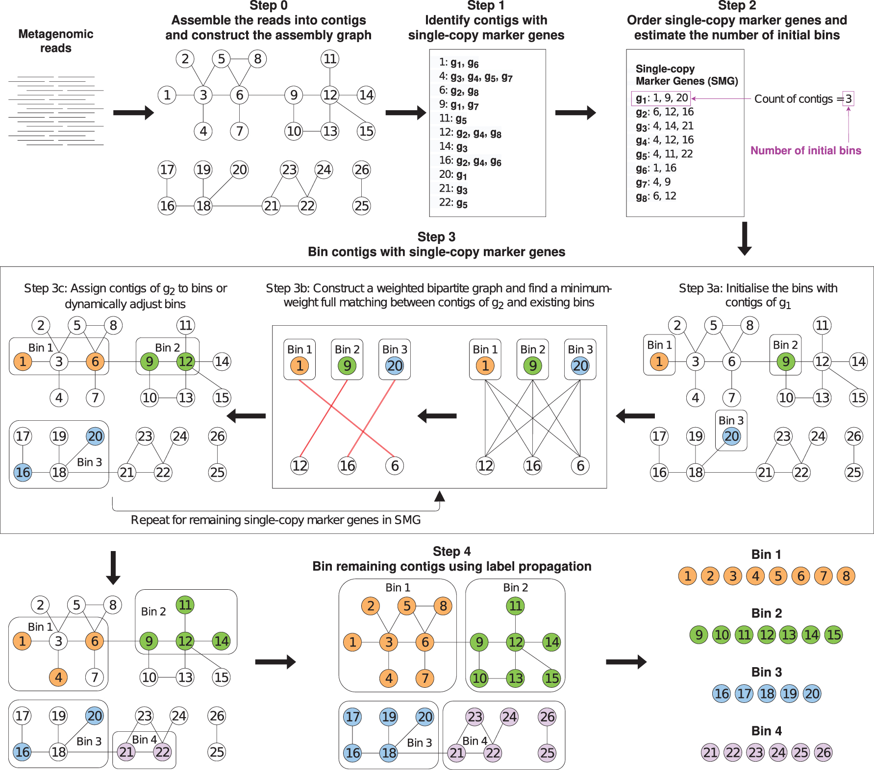
MetaCoAG workflow.

2.1. Step 0: Assemble reads into contigs and construct the assembly graph

A preprocessing step consists of assembling the reads into contigs using a metagenomic assembler and obtaining the assembly graph. Metagenomic assemblers first use graph models to connect overlapping reads or k-mers and infer contigs as nonbranching paths. After graph simplification, the vertices represent contigs and edges represent connections between contigs in the assembly graph. Here, we use the popular metagenomic assembler metaSPAdes (Nurk et al., 2017) to derive the contigs and assembly graph, which are used as inputs to MetaCoAG. Note that the assembly graphs can also be obtained similarly using other metagenomic assemblers such as MEGAHIT (Li et al., 2015) and metaFlye (Kolmogorov et al., 2020).

2.2. Step 1: Identify contigs with single-copy marker genes

Single-copy marker genes are special marker genes that appear exactly once in a bacterial genome and are conserved in the majority of bacterial genomes (Dupont et al., 2012; Albertsen et al., 2013; Wu et al., 2014). We use FragGeneScan (Rho et al., 2010) and HMMER (Eddy, 2011) to identify the contigs, which contain each single-copy marker gene (as shown in Step 1 of Fig. 1). A single-copy marker gene is considered to be contained in a contig if more than 50% of the gene length is aligned to this contig. In an ideal assembly, a single-copy marker gene from one species should only be contained in one contig from this species.

Similar to approaches such as MaxBin (Wu et al., 2014), MaxBin2 (Wu et al., 2015), and SolidBin (Wang et al., 2019), MetaCoAG uses single-copy marker genes to distinguish contigs belonging to different species, that is, if multiple contigs contain the same single-copy marker gene, they should belong to different species, respectively.

2.3. Step 2: Order single-copy marker genes and estimate the number of initial bins

For a given single-copy marker gene, the contigs containing this marker gene should come from different species (e.g., if two contigs contain the same marker gene, then the two contigs should belong to two different species). In the ideal case, if we have a near-perfect assembly, the number of contigs that contain the same single-copy marker gene should be equal to the number of species present in the sample. However, in reality, assemblies can be fragmented and erroneous, which make it challenging to recover all single-copy marker genes and, hence, can lower the counts of contigs containing each single-copy marker gene.

To get a better estimate of the number of species, we obtain the counts of contigs containing each single-copy marker gene. We also record the single-copy marker genes found in each contig. For a single-copy marker gene, the number of contigs that it can distinguish is the number of contigs containing this gene. Therefore, we order all the single-copy marker genes according to the descending order of the number of contigs containing them (as shown in Step 2 of Fig. 1). We refer to this list of ordered marker genes as SMG, where a single-copy marker gene g_i has a set of contigs $C (g_{i})$ containing g_i. The number of initial bins is empirically set to be the number of contigs that contain the first gene in SMG, to recover the maximum number of species possible from the marker gene information (as shown in Step 2 of Fig. 1).

2.4. Step 3: Bin contigs with single-copy marker genes

2.4.1. Step 3a: Initialize bins

We initialize the bins using the contigs of the first single-copy marker gene g₁ in SMG; that is, we initialize a new bin B for each contig in $C (g_{1})$ (as shown in Step 3a of Fig. 1). We define the initialized set of bins as BINS. Please note that the number of bins $| B I N S |$ may change during the binning process.

2.4.2. Calculating composition and coverage similarities

Previous studies on metagenomic binning have used genomic signatures as they follow species-specific patterns (Deschavanne et al., 1999; Wu et al., 2014). The most commonly used genomic signatures to characterize composition information are tetranucleotide frequencies (136 canonical 4-mers, also known as tetramers; Alneberg et al., 2014; Wu et al., 2014, 2015; Kang et al., 2019; Wang et al., 2019; Nissen et al., 2021). For each contig c, we normalize the tetranucleotide frequencies using its total number of tetranucleotides to obtain the normalized tetranucleotide frequency vector, $t e t r a (c)$ . We obtain the tetranucleotide composition distance between contigs c and $c'$ as $d_{t e t r a} (c, c') = d i s t_{E} (t e t r a (c), t e t r a (c'))$ , where $d i s t_{E}$ is the Euclidean distance function.

We use the same formula proposed by Wu et al. (Wu et al., 2014) to estimate how similar c and $c'$ are (i.e., belonging to the same species) based on their composition, $S_{c o m p} (c, c')$ as shown in Equation (1).

$N_{i n t r a}$ and $N_{i n t e r}$ are Gaussian distributions with $μ_{i n t r a}$ , $σ_{i n t r a}$ , $μ_{i n t e r}$ , and $σ_{i n t e r}$ set according to the latest values of MaxBin 2.2.7 (Wu et al., 2015), which have been calculated by analyzing the Euclidean distance between the tetranucleotide frequencies of pairs of sequences sampled from the same genome (intra) and different genomes (inter). If the distance is lower between two sequences, they are more similar, and are more likely to belong to the same genome.

We use the coverage information of the contigs as coverage carries important information about the abundance of species and has been used in previous metagenomic binning studies (Albertsen et al., 2013; Wu et al., 2014; Kang et al., 2019; Wang et al., 2019; Nissen et al., 2021). Shotgun sequencing has shown to follow the Lander–Waterman model (Lander and Waterman, 1988) and the Poisson distribution has been used to obtain the sequencing coverage of nucleotides and applied in metagenomic binning (Wu and Ye, 2011; Wu et al., 2014). Modifying the definition found in Wu et al. (2014), we estimate how similar c and $c'$ are in terms of their coverage values in each sample, $S_{c o v} (c, c')$ as shown in Equation (2). $S_{c o v} (c, c') = min (\prod_{n = 1}^{M} P o i s s o n (c o v_{n} (c) | c o v_{n} (c')), \prod_{n = 1}^{M} P o i s s o n (c o v_{n} (c') | c o v_{n} (c)))$ (2)

Here, $c o v_{n} (c)$ and $c o v_{n} (c')$ refer to the coverage values of the contigs c and $c'$ , respectively, in the sample n, where M is the total number of samples. Poisson is the Poisson probability mass function.

2.4.3. Step 3b: Construct a weighted bipartite graph and find a minimum-weight full matching

In the previous steps, we have used single-copy marker genes to identify pairs of contigs that belong to different species. Remind that contigs in different bins in BINS are expected to belong to different species and contigs in $C (g_{i})$ are also expected to belong to different species. However, there is no measurement to measure how likely a contig c in $C (g_{i})$ belongs to an existing bin B in BINS. Therefore, we introduce a bipartite graph between $C (g_{i})$ and BINS and propose a weight $w_{c 2 B} (c, B)$ between a contig c in $C (g_{i})$ and an existing bin B in BINS as shown in Equation (3). $w_{c 2 B} (c, B) = \frac{\sum_{c' \in B} w_{c 2 c} (c, c')}{| B |}$ (3)

In Equation (3), $w_{c 2 c} (c, c')$ is the weight that measures how likely a pair of contigs c and $c'$ belong to the same species and is computed using Equation (4). $S_{c o m p} (c, c')$ and $S_{c o v} (c, c')$ are calculated according to Equations (1) and (2), respectively. $w_{c 2 c} (c, c') = - (l o g (S_{c o m p} (c, c')) + l o g (S_{c o v} (c, c')))$ (4)

Now, we find a minimum-weight full matching (minimum-cost assignment; Karp, 1980) for the above bipartite graph between $C (g_{i})$ and BINS where every contig c in $C (g_{i})$ will get paired with exactly one bin B in BINS (as shown in Step 3b of Fig. 1). For this purpose, we use the minimum-weight full matching algorithm implemented in the NetworkX (Hagberg et al., 2008) python library, which is based on the algorithm proposed by Karp (1980) and the time complexity is $O (| C (g_{i}) | \times | B I N S | \times l o g (| B I N S |))$ .

In the next step, we will see how we can assign the contigs to existing bins based on the minimum-weight full matching we have obtained.

2.4.4. Step 3c: Assign contigs to existing bins and dynamically adjust bins

Previous studies have observed that contigs connected to each other in the assembly graph are more likely to belong to the same taxonomic group (Barnum et al., 2018; Mallawaarachchi et al., 2020a). While $w_{c 2 B} (c, B)$ considers both composition and coverage information, the assembly graph has not yet been incorporated into the binning process. Therefore, we introduce $d_{g r a p h} (c, B)$ to measure how well contig c is connected to contigs in bin B within the assembly graph. Specifically, $d_{g r a p h} (c, B)$ is defined as the average length of the shortest-path distances between contig c and all the contigs in bin B in the assembly graph. Note that both $w_{c 2 B} (c, B)$ and $d_{g r a p h} (c, B)$ will be used to assign contigs to existing bins or dynamically adjust the bins.

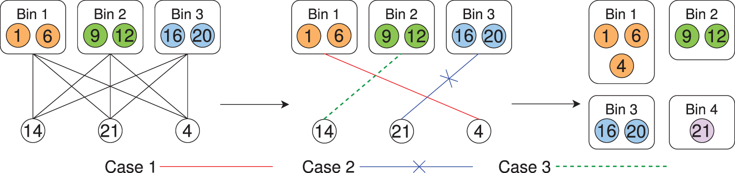
We define the thresholds intraspecies weight $w_{i n t r a} = - (l o g (p_{i n t r a})) \times M$ and interspecies weight, $w_{i n t e r} = - (l o g (p_{i n t e r})) \times M$ , where M is the number of samples in the dataset. Each candidate pair $(c, B)$ obtained from the minimum-weight full matching falls under one of the following three cases (refer Fig. 2).

FIG. 2.

Cases 1, 2, and 3 in assigning contigs to existing bins or adjusting bins.

Case 1: If the weight of the candidate pair $w_{c 2 B} (c, B)$ is less than or equal to $w_{i n t r a}$ and the average distance $d_{g r a p h} (c, B)$ is less than or equal to $d_{l i m i t}$ , then contig c will be assigned to bin B, that is, $B \leftarrow B \cup {c}$ (e.g., contig 4 and Bin 1 in Fig. 2).

Case 2: If the weight of the candidate pair $w_{c 2 B} (c, B)$ is greater than $w_{i n t e r}$ and the average distance $d_{g r a p h} (c, B)$ is greater than $d_{l i m i t}$ , then a new bin $B'$ is created and contig c is assigned to that new bin, that is, $B' = {c}$ and $B I N S \leftarrow B I N S \cup {B'}$ (e.g., contig 21 in Fig. 2).

Case 3: If $w_{c 2 B} (c, B)$ and $d_{g r a p h} (c, B)$ satisfy neither Case 1 nor Case 2, then contig c will not be assigned to any bin (e.g., contig 14 in Fig. 2).

The default values for parameters $p_{i n t r a}$ , $p_{i n t e r}$ , and $d_{l i m i t}$ were chosen empirically and set to 0.1, 0.01 and 20, respectively. Now, we iteratively perform Steps 3b and 3c to process all the contigs containing single-copy marker genes (as shown in Step 3b and 3c of Fig. 1). The remaining challenge is to bin the contigs, which do not contain single-copy marker genes, which will be addressed in Step 4.

2.5. Step 4: Bin remaining contigs using label propagation

After we bin the contigs with single-copy marker genes, each such contig receives a label corresponding to its bin. Now, we will propagate labels from these contigs to other unlabeled contigs within the same connected component (as shown in Step 4 of Fig. 1).

2.5.1. Step 4a: Propagate labels within connected components

MetaCoAG uses composition, coverage, and distance information from the assembly graph to propagate labels from labeled contigs to the unlabeled contigs located within the same connected components. More specifically, for each unlabeled long contig c (at least 1000 bp long because short contigs result in unreliable composition and coverage information) directly connected or connected via short contigs to a labeled contig $c'$ , MetaCoAG computes a candidate propagation action $(c', c, d (c, c'), w_{c 2 B} (c, B'))$ , where $d (c, c')$ is the shortest distance between c and $c'$ using only unlabeled vertices, and $w_{c 2 B} (c, B')$ is computed according to Equation (3), where $B'$ is the bin to which contig $c'$ is assigned. Given two candidate propagation actions $(a, b, d, w)$ and $(a', b', d', w')$ , $(a, b, d, w)$ has a higher priority than $(a', b', d', w')$ if $d < d'$ or ( $w < w'$ and $d = d'$ ).

MetaCoAG iteratively selects the candidate propagation action with the highest priority and executes the corresponding label propagation. If a contig to be labeled contains single-copy marker genes, the relevant candidate propagation action is executed if the single-copy marker genes of the contig are not present in the intended bin. We restrict the depth of the search for labeled contigs in this step to 10.

2.5.2. Step 4b: Propagate labels across different components

Note that some components in the assembly graph may not have any labeled contigs, and we need to propagate labels from labeled bins to unlabeled contigs across components. Calculating pair-wise weights $w_{c 2 c} (c, c')$ for all the remaining contigs becomes time-consuming. Hence, for each bin B, we create a representative contig $c (B)$ , which has a composition profile and a coverage profile calculated by averaging the normalized tetranucleotide frequency vectors and coverage vectors of all the contigs in bin B, respectively. These profiles will provide a better representation of the composition and coverage of the bins. Then, for each unlabeled contig c, MetaCoAG identifies a bin B that minimizes $w_{c 2 c} (c, c (B))$ , which is calculated according to Equation 4, and assigns contig c into that bin B.

This propagation is limited to long contigs (at least 1000 bp long by default). If an unlabeled contig contains single-copy marker genes, it is assigned to bin B that minimizes $w_{c 2 c} (c, c (B))$ if the single-copy marker genes of the contig are not present in bin B. Then, Step 4a is performed again to further propagate labels.

2.5.3. Step 4c: Postprocessing

In this step, we will make final adjustments on the current bins. Two bins B and $B'$ are mergeable if they have no common marker genes and $w_{c 2 c} (c (B), c (B'))$ [calculated by Equation (4)] is upper bounded by $w_{i n t r a}$ (defined in Step 3c). Then, MetaCoAG creates a graph where vertices denote current bins, and edges between two vertices denote that the corresponding two bins are mergeable. Now, we use the python implementation of the igraph (Csardi and Nepusz, 2006) library to find maximal cliques (maximal_cliques) in this graph and merge the bins found in each maximal clique. After merging bins, we also remove the bins that contain less than one third (set by default) of the single-copy marker genes. Finally, MetaCoAG outputs the bins along with their corresponding contigs.

3. EXPERIMENTAL SETUP

3.1. Datasets and tools

3.1.1. Simulated datasets

We evaluated the binning performance on the simulated simHC+ dataset (Wu et al., 2014), which consists of 100 bacterial species. Paired-end reads were simulated using InSilicoSeq (Gourlé et al., 2018) with the predefined MiSeq error model.

3.1.2. CAMI2 toy human microbiome project datasets

We used the simulated metagenome data from the toy Human Microbiome Project dataset of the second CAMI challenge (Meyer et al., 2022). Metagenomes with HiSeq reads were simulated from five different body sites of the human host as follows.

Urogenital tract—referred as CAMI UG

Skin—referred as CAMI Skin

Oral cavity—referred as CAMI Oral

Gastrointestinal tract—referred as CAMI GI

Airways—referred as CAMI Airways

3.1.3. Real datasets

We used the following three real datasets from the National Center for Biotechnology Information (NCBI) to evaluate the binning performance on real-world metagenomic data.

Preborn infant gut metagenome (Sharon et al., 2013) with 18 samples (NCBI accession number SRA052203), referred as Sharon

Metagenomics of the Chronic Obstructive Pulmonary Disease (COPD) Lung Microbiome (Cameron et al., 2016) with 18 samples (NCBI BioProject number PRJEB9034), referred as COPD

Human metagenome sample from tongue dorsum of a participant from the Deep Whole-Genome Sequencing (WGS) Human Microbiome Project (HMP) clinical samples (Lloyd-Price et al., 2017) with 8 samples (NCBI accession number SRX378791), referred as Deep HMP TD.

Refer to Table 1 for further details of all the datasets.

Table 1.

Further Information of the Datasets

Dataset	No. of samples	Read length (bp)	Assembly size (Mb)	Total no. of assembled contigs	No. of contigs longer than 1000 bp	No. of edges in the assembly graph	Density ^a of the assembly graph	N50 (bp)
simHC+	1	301	314.23	15,729	6706	31,199	1.984	154,030
CAMI UG	9	150	336.69	192,679	49,927	40,861	0.212	8081
CAMI Skin	10	150	639.91	600,508	139,217	51,139	0.085	1965
CAMI Oral	10	150	517.35	493,149	96,079	87,910	0.178	2405
CAMI GI	10	150	507.09	255,722	75,913	39,240	0.153	9319
CAMI Airways	10	150	664.49	729,063	142,477	49,531	0.067	1506
Sharon	18	100	45.06	37,164	7067	20,328	0.547	5609
COPD	18	151	343.52	452,600	67,753	73,519	0.162	1042
Deep HMP TD	8	101	158.099	227,635	28,164	86,250	0.379	1123

Density of the graph is calculated as (the number of edges)/(the number of vertices).

CAMI, Critical Assessment of Metagenomic Interpretation; CAMI GI, CAMI Urogenital; CAMI UG, CAMI Gastrointestinal; COPD, Chronic Obstructive Pulmonary Disease.

3.1.4. Tools used

We used the popular metagenomic assembler metaSPAdes (Nurk et al., 2017; from SPAdes version 3.15.2 (Bankevich et al., 2012)) to assemble reads into contigs and obtain the assembly graphs. For the datasets containing multiple samples, the contigs and assembly graph were obtained by coassembling the reads from all the samples together. The mean coverage of each contig in each sample was calculated using CoverM (available at https://github.com/wwood/CoverM).

MetaCoAG was benchmarked against the binning tools MaxBin2 (version 2.2.7; Wu et al., 2015), MetaBAT2 (version 2.12.1; Kang et al., 2019), and Vamb (version 3.0.1; Nissen et al., 2021). MaxBin2 uses probabilistic models and an Expectation Maximization (EM) algorithm to iteratively bin the contigs based on their normalized tetranucleotide frequencies and coverage profiles. MetaBAT2 uses normalized tetranucleotide frequency scores and coverage profiles to construct a graph and performs clustering on this graph to bin contigs. Vamb makes use of deep variational autoencoders to encode normalized tetranucleotide frequencies and coverage profiles of contigs and performs clustering on the encoded information. MaxBin2 was run in its default settings, MetaBAT2 with the parameter -m 1500 and Vamb in coassembly mode (for a fair comparison with other tools) with the parameter - -min-fasta 200000 as per authors. The commands used to run these tools can be found in Figure 3.

FIG. 3.

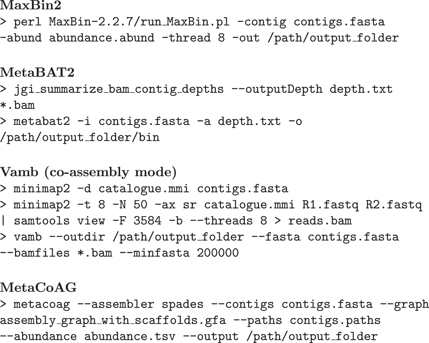
Commands used to run the different binning tools.

The binning results were evaluated using the tools Assessment of Metagenome BinnERs (AMBER) (Meyer et al., 2018; version 2.0.2), CheckM (Parks et al., 2015; version 1.1.3), and Genome Taxonomy Database-Toolkit (GTDB-Tk) (Chaumeil et al., 2019; version 1.5.0).

3.2. Evaluation metrics

We used Minimap2 (Li, 2018) to map the contigs to the reference genomes and determine their ground truth for the simHC+ dataset as the reference genomes of the underlying species were available. With this ground truth annotation of contigs, we used AMBER (Meyer et al., 2018) to assess the binning results of the simHC+ dataset. We define the AMBER F1-score as follows. $A M B E R F 1 - s c o r e = 2 \times \frac{p r e c i s i o n \times r e c a l l}{p r e c i s i o n + r e c a l l}$ (5)

where $p r e c i s i o n = A M B E R p u r i t y$ and $r e c a l l = A M B E R c o m p l e t e n e s s$ .

For all the datasets, we determined the completeness and contamination of each bin produced by all the binning tools using CheckM (Parks et al., 2015). We define the CheckM F1-score for each bin as follows. $C h e c k M F 1 - s c o r e = 2 \times \frac{p r e c i s i o n \times r e c a l l}{p r e c i s i o n + r e c a l l}$ (6)

where $p r e c i s i o n = \frac{1}{1 + C h e c k M c o n t a m i n a t i o n}$ and $r e c a l l = C h e c k M c o m p l e t e n e s s$ .

Furthermore, considering purity (precision) and completeness based on the CheckM results, we counted the number of high-quality bins (bins with $>$ 80% completeness and $>$ 90% purity), medium-quality bins (bins with $>$ 50% completeness and $>$ 80% purity), and low-quality bins (bins which are not considered as high-quality or medium-quality).

4. RESULTS AND DISCUSSION

4.1. Benchmarks using simHC+ dataset

We first benchmarked MetaCoAG against two popular contig-binning tools, MaxBin2 (Wu et al., 2015) and MetaBAT2 (Kang et al., 2019), on the simulated dataset simHC+ (Wu et al., 2014).* We evaluated the binning results of the simHC+ dataset produced by all the tools using the two popular evaluation tools AMBER (Meyer et al., 2018) and CheckM (Parks et al., 2015). AMBER assesses the quality of bins based on the ground truth annotations provided and CheckM assesses the quality of bins based on sets of single-copy marker genes. We analyzed the purity, completeness, and F1-score of the binning results calculated by AMBER (at the nucleotide level) and CheckM (refer to Table 2 for exact values).

Table 2.

AMBER and CheckM Evaluation Results for the simHC+ Dataset

Evaluation criteria	MaxBin score (%)	MetaBAT2 score (%)	MetaCoAG score (%)
Average purity per bin (AMBER)	90.36	98.30	91.07
Average purity per bin (CheckM)	97.25	100.0	97.55
Average completeness per bin (AMBER)	79.34	13.02	82.73
Average completeness per bin (CheckM)	77.51	29.59	87.17
F1-score per bin (AMBER)	84.50	23.00	86.70
F1-score per bin (CheckM)	80.64	37.25	89.44
Accuracy (AMBER)	77.07	14.38	84.46
Binned fraction (AMBER)	84.90	14.79	92.04

Bold values are the best evaluation results.

MetaCoAG has recovered bins with a better trade-off between purity and completeness when compared to other binning tools (Fig. 4a). This better trade-off is demonstrated from the best F1-score results produced by MetaCoAG with a median F1-score of 95.69% from AMBER and a median F1-score of 98.48% from CheckM (Fig. 4b and c, respectively, where each point denotes a bin) when compared with other binning tools. Furthermore, MetaCoAG has recovered the highest number of high-quality bins (69 bins) and the lowest number of low-quality bins (13 bins; refer to Table 4).

FIG. 4.

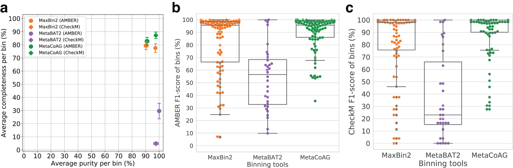
Binning results of the simHC+ dataset: (a) Average completeness per bin versus average purity per bin from AMBER and CheckM results of each binning tool, (b) Swarm plot with overlaid box plot for the AMBER F1-score of the bins produced by each binning tool and (c) Swarm plot with overlaid box plot for the CheckM F1-score of the bins produced by each binning tool.

Many existing binning tools assume that the oligonucleotide composition and coverage are conserved across the genome. Hence, it is challenging for such tools to bin species with high variance in oligonucleotide composition and/or coverage. In Figure 5, we visualize and compare the binning results of MaxBin2 and MetaCoAG^† against the ground truth for the following species, Pseudomonas putida and Arthrobacter arilaitensis. The species Pseudomonas putida has a high variance in oligonucleotide composition (standard deviation $>$ 0.015 for the tetranucleotide composition of its contigs) and thus MaxBin2 has split this species into multiple bins incorrectly (refer to Fig. 5a). The species Arthrobacter arilaitensis has a high variance in genome coverage (standard deviation $>$ 50 × for the coverages of its contigs) and thus MaxBin2 has misbinned some high-coverage contigs into other species with high coverage (refer to Fig. 5b). However, MetaCoAG has been able to recover these species with high F1-score values, for example, improving the F1 score for Pseudomonas putida from 59.78% to 99.56% and improving the F1-score for Arthrobacter arilaitensis from 97.65% to 98.99%. Despite the high variance in oligonucleotide composition and coverage, MetaCoAG has been able to recover these species accurately, thanks to the additional connectivity information from the assembly graph.

FIG. 5.

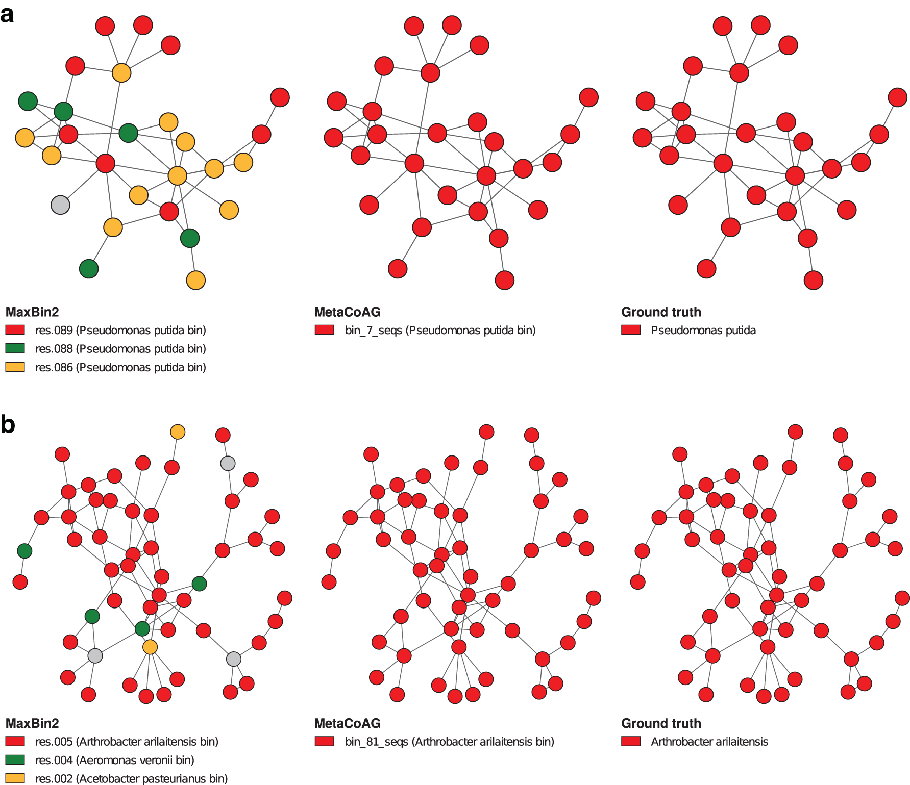
Visualization of the binning results of simHC+ dataset from MaxBin2 and MetaCoAG for a species with (a) high variance in oligonucleotide composition (standard deviation >0.015) and (b) high variance in coverage (standard deviation >50 × ). Gray color nodes denote contigs, which were binned to bins other than the ones specified in the figure.

Another major challenge faced by most of the existing metagenomic binning tools is how to accurately separate contigs of species belonging to the same genus, where such species tend to have similar oligonucleotide composition and appear in similar abundances. For example, the three species, S. pneumoniae, S. thermophilus, and S. suis from simHC+ belong to the Streptococcus genus, and they have very similar oligonucleotide composition and coverage values (refer to Fig. 6a). Not surprisingly, contigs from these three species were incorrectly binned by MaxBin2 and even ignored by MataBAT2 because they share similar composition and coverage profiles (refer to Fig. 6b).

FIG. 6.

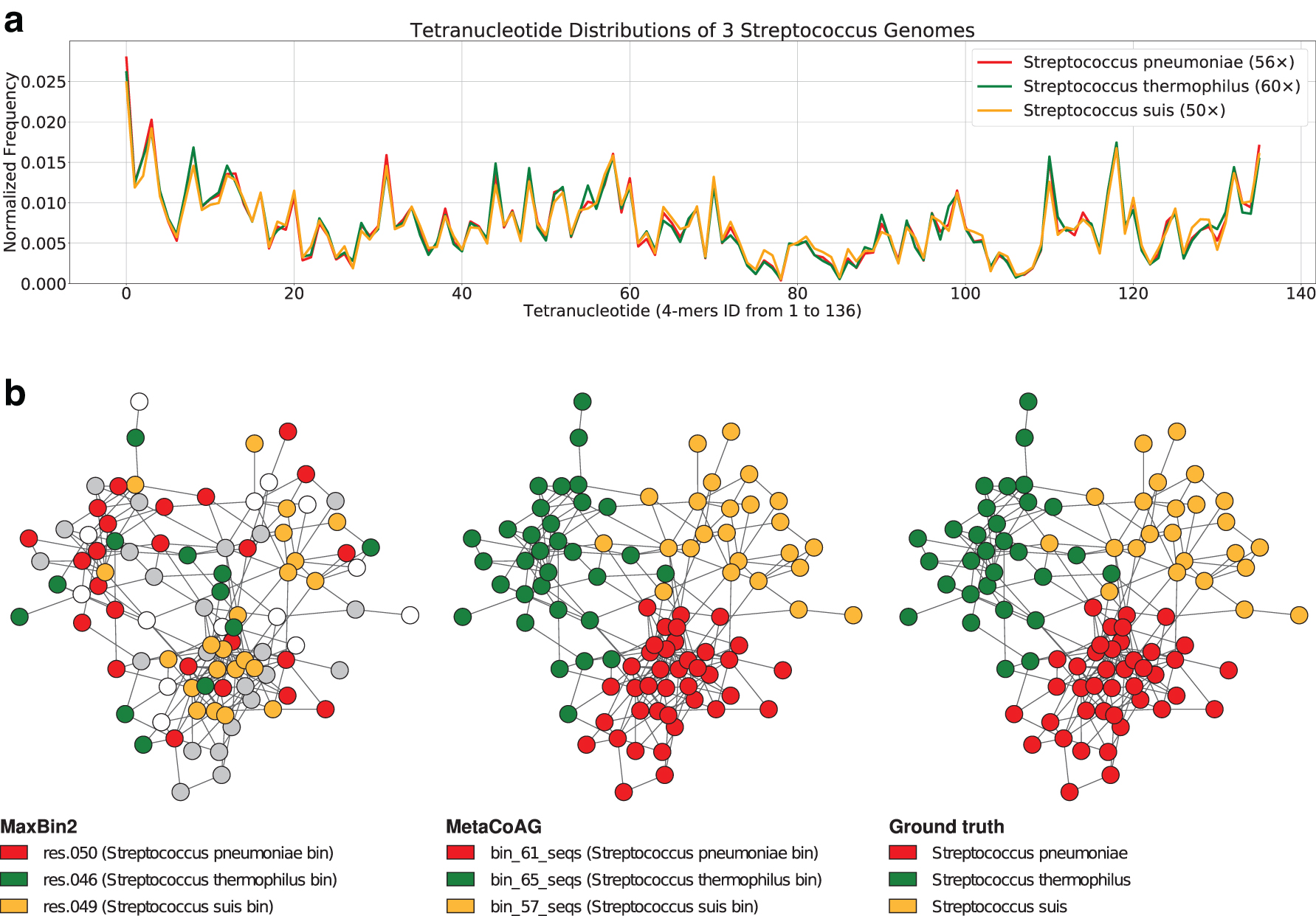
Visualization of the (a) tetranucleotide composition and (b) binning results of three Streptococcus genomes in the simHC+ dataset.

On the contrary, MetaCoAG was able to accurately bin most of the contigs from these three species because they naturally form three subgraphs in the assembly graph (refer to Fig. 6b), thus improving the F1-scores of S. pneumoniae from 46.51% to 93.40%, S. thermophilus from 49.97% to 95.67%, and S. suis from 72.39% to 95.95%. Figure 6b demonstrates that the use of assembly graph in MetaCoAG can assist in separating species, despite the high similarity in oligonucleotide composition and coverage of certain species. Furthermore, we observed that the assembly graphs help MetaCoAG to bin species with high variance of intraspecies oligonucleotide composition and coverage profiles while most existing tools suffer from the assumption that the oligonucleotide composition and coverage are conserved within the same species.

4.2. Benchmarks using CAMI2 toy human microbiome project datasets

We benchmarked MetaCoAG against MaxBin2 (Wu et al., 2015), MetaBAT2 (Kang et al., 2019), and Vamb (Nissen et al., 2021) on five publicly available datasets from the toy Human Microbiome Project dataset of the second CAMI challenge (Meyer et al., 2022; refer to Table 1 for further details of the CAMI datasets). Multiple samples from each dataset were coassembled together to obtain the final contigs for binning.

We evaluated the binning results of the CAMI datasets using CheckM (Parks et al., 2015) and reported the F1-score of the bins produced by all the binning tools (refer to equation 6). Figure 7a–e shows that overall MetaCoAG has achieved the best binning results among all the binning tools. The overall median F1-scores averaging from all 5 CAMI datasets for MetaCoAG, MaxBin2, MetaBAT2, and Vamb are 86.77%, 75.41%, 1.57%, and 33.30%, respectively. More specifically, MetaCoAG has recovered more complete bins with higher purity and lower contamination when compared to other tools.

FIG. 7.

Swarm plots with overlaid box plots for the F1-score from CheckM results of the CAMI datasets: (a) CAMI UG, (b) CAMI Skin, (c) CAMI Oral, (d) CAMI GI, and (e) CAMI Airways. Each point denotes a bin. CAMI, Critical Assessment of Metagenomic Interpretation; CAMI GI, CAMI Urogenital; CAMI UG, CAMI Gastrointestinal.

MetaCoAG produced the highest numbers of high-quality and medium-quality bins combined together for all the CAMI datasets (refer to Table 4). Note that only MaxBin2 outperforms MetaCoAG in terms of the number of high-quality bins just for the CAMI GI dataset. This dataset had a low density in its assembly graph (refer to Table 1 for density of the assembly graph), which prevented MetaCoAG from making full use of the assembly graphs.

4.3. Benchmarks using real datasets

We benchmarked MetaCoAG against MaxBin2 (Wu et al., 2015), MetaBAT2 (Kang et al., 2019) and Vamb (Nissen et al., 2021) on three real metagenomic datasets; Sharon (Sharon et al., 2013), COPD (Cameron et al., 2016), and Deep HMP TD (Lloyd-Price et al., 2017). Similar to the simHC+ and CAMI datasets, we use CheckM (Parks et al., 2015) to evaluate the bins produced by all the binning tools and identify high-quality bins.

Figure 8 shows that MetaCoAG has also achieved the best binning result in terms of the median F1-score for the real datasets. For the Sharon dataset, MetaCoAG records a median F1-score of 99.24% while the second-best tool (Vamb) has a median F1-score of 83.88%. For the COPD dataset, MetaCoAG records a median F1-score of 75.68% while the second-best tool (MaxBin2) has a median F1-score of 25.13%. For the Deep HMP TD dataset, MetaCoAG records a median F1-score of 76.34% while the second-best tool (MaxBin2) has a median F1-score of 37.40%. Furthermore, MetaCoAG has produced the highest number of high-quality bins for all the real datasets (refer to Table 4).

FIG. 8.

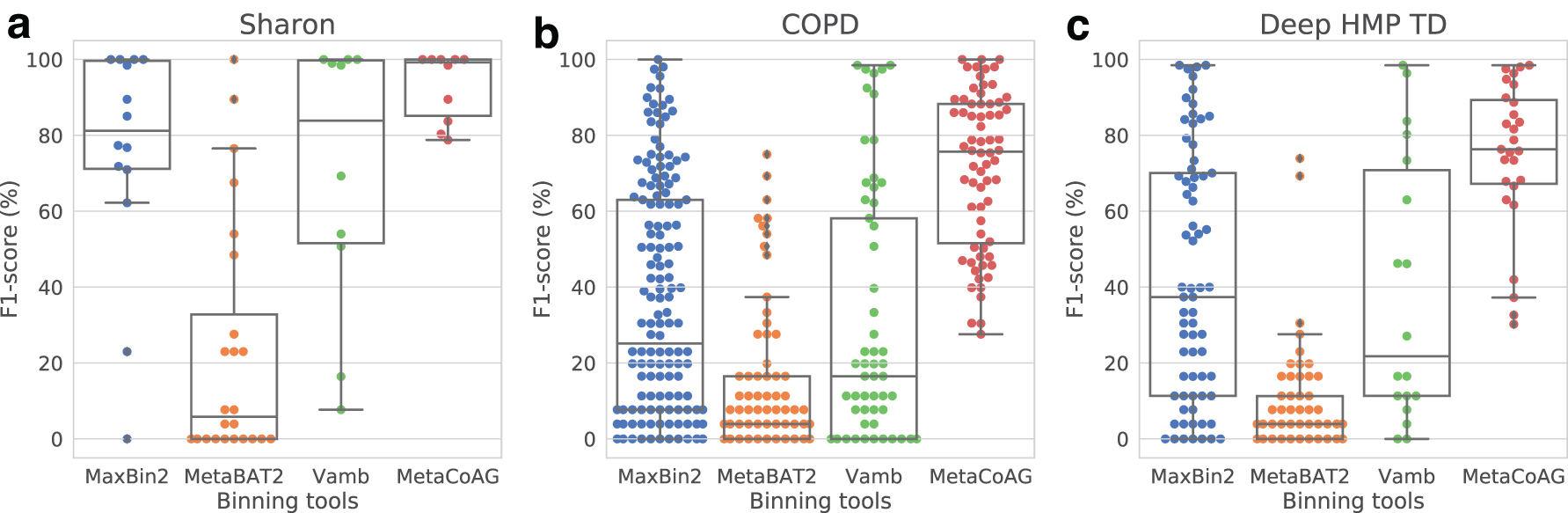
Swarm plots with overlaid box plots for the F1-score from CheckM results of the real datasets: (a) Sharon, (b) COPD, and (c) Deep HMP TD. Each point denotes a bin. COPD, Chronic Obstructive Pulmonary Disease.

We used GTDB-Tk (Chaumeil et al., 2019) to annotate all the high-quality bins produced by the three best-performing tools; MetaCoAG, MaxBin2, and Vamb^‡ for the real datasets. Then we compared the taxonomic annotations (up to the species level) with the analysis results reported by the authors of these datasets as shown in Table 3. According to Table 3, MetaCoAG achieves the best consistency with the original analysis reported by the authors. In the Sharon dataset, the five most abundant species reported according to the authors (Sharon et al., 2013), Staphylococcus epidermidis, Enterococcus faecalis, Cutibacterium avidum, Peptoniphilus lacydonensis, and Staphylococcus aureus, have been successfully identified by all the three binning tools. However, Vamb missed Staphylococcus hominis, which is reported as a rare species in the Sharon dataset (Sharon et al., 2013). Moreover, MetaCoAG is the only tool that is able to recover Leuconostoc citreum, which is also identified as a rare species in the Sharon dataset (Sharon et al., 2013). These results denote the ability of MetaCoAG to recover rare species in real metagenomics samples that are ignored by other binning tools.

Table 3.

GTDB-Tk Annotations of High-Quality Species for the Real Datasets

Dataset	Species	MaxBin2	Vamb	MetaCoAG	Present in original analysis
Sharon	Cutibacterium avidum	✓	✓	✓	✓
	Enterococcus faecalis	✓	✓	✓	✓
	Peptoniphilus lacydonensis	✓	✓	✓	✓
	Staphylococcus aureus	✓	✓	✓	✓
	Staphylococcus epidermidis	✓	✓	✓	✓
	Staphylococcus hominis	✓	✗	✓	✓
	Leuconostoc citreum	✗	✗	✓	✓
COPD^a	Peptostreptococcus sp.	✓	✓	✓	✓
	SR1 bacterium human oral taxon HOT-345	✓	✓	✓	✗ ^b
	Prevotella pallens	✗	✓	✓	✓
	Haemophilus sputorum	✗	✓	✓	✓
	Herbaspirillum huttiense	✗	✓	✓	✓
	Capnocytophaga gingivalis	✓	✗	✓	✓
	Capnocytophaga leadbetteri	✓	✗	✓	✓
	Lancefieldella sp000564995	✓	✗	✓	✓
	Actinomyces graevenitzii	✓	✗	✗	✓
	Actinomyces oris	✓	✗	✗	✓
	Anaeroglobus micronuciformis	✓	✗	✗	✗
	Eubacterium sulci	✗	✗	✓	✓
	Prevotella shahii	✗	✗	✓	✓
	Prevotella histicola	✗	✗	✓	✓
	Lachnospiraceae bacterium oral taxon 096	✗	✗	✓	✗ ^b
Deep HMP TD^a	Actinomyces graevenitzii	✓	✓	✓	✓
	Saccharimonadaceae TM7x sp900557595	✓	✓	✓	✗ ^b
	Neisseria subflava_C	✓	✗	✓	✓
	Prevotella pallens	✓	✗	✓	✓
	Anaeroglobus micronuciformis	✓	✗	✓	✗
	Actinomyces sp. ICM47	✓	✗	✓	✓
	Lancefieldella sp000564995	✓	✗	✗	✗
	Eubacterium_B sulci	✗	✗	✓	✓

✓ denotes that the species is present and ✗ denotes that the species is absent in the result/analysis. Bold items match the original analysis, whereas the gray colored items do not match the original analysis.

The species were determined based on the most abundant genera presented.

These species were added to National Center for Biotechnology Information taxonomy in year 2020 (Schoch et al., 2020), which is after the relevant analysis (Cameron et al., 2016; Lloyd-Price et al., 2017).

Vamb, Variational autoencoder for metagenomic binning.

Table 4.

The Number of High-Quality, Medium-Quality, and Low-Quality Bins

Dataset	Binning tool	No. of bins detected	High-quality	Medium-quality	Low-quality
simHC+	MaxBin2	95	59	11	25
	MetaBAT2	32	4	4	24
	MetaCoAG	90	69	8	13
CAMI UG	MaxBin2	98	49	17	32
	MetaBAT2	202	5	12	185
	Vamb	100	34	10	56
	MetaCoAG	83	50	17	16
CAMI Skin	MaxBin2	176	42	30	104
	MetaBAT2	240	0	5	235
	Vamb	167	36	15	116
	MetaCoAG	106	49	33	24
CAMI Oral	MaxBin2	137	54	24	59
	MetaBAT2	152	1	7	144
	Vamb	176	45	19	112
	MetaCoAG	106	58	19	29
CAMI GI	MaxBin2	127	59	22	46
	MetaBAT2	389	4	9	376
	Vamb	156	44	14	98
	MetaCoAG	113	57	28	28
CAMI Airways	MaxBin2	155	32	26	97
	MetaBAT2	205	1	2	202
	Vamb	173	20	14	139
	MetaCoAG	96	33	29	34
Sharon	MaxBin2	14	6	2	6
	MetaBAT2	24	2	2	20
	Vamb	10	5	1	4
	MetaCoAG	10	7	3	0
COPD	MaxBin2	156	9	24	123
	MetaBAT2	76	0	2	74
	Vamb	61	6	7	48
	MetaCoAG	68	17	25	26
Deep HMP TD	MaxBin2	69	8	15	46
	MetaBAT2	61	0	1	60
	Vamb	29	2	3	13
	MetaCoAG	27	8	9	10

Bold values are the best results.

In the COPD dataset, there is a larger discrepancy among MaxBin2, Vamb, and MetaCoAG. Only two species, Peptostreptococcus sp. and SR1 bacterium human oral taxon HOT-345, have been identified by all the three binning tools. SR1 bacterium human oral taxon HOT-345 and Lachnospiraceae bacterium oral taxon 096 have been added to NCBI taxonomy recently (Schoch et al., 2020) and hence are not found in the original analysis (Cameron et al., 2016). Compared to MetaCoAG, MaxBin2 failed to identify three species Prevotella pallens, Prevotella shahii, and Prevotella histicola while Vamb only identified P. pallens under the genus Prevotella. Similarly, Vamb failed to identify two species, Capnocytophaga gingivalis and Capnocytophaga leadbetteri, both of which are identified by MaxBin2 and MetaCoAG. Moreover, the species Anaeroglobus micronuciformis only identified by MaxBin2 was not present in the top 50 genera ranked by abundance in the original analysis (Cameron et al., 2016), which is likely to be a false-positive.

In the Deep HMP TD dataset, the species identified by MetaCoAG show the best consistency with the original analysis (Lloyd-Price et al., 2017), while being the only tool to identify the species from the genus Eubacterium. These results demonstrate that MetaCoAG has been able to recover species in real metagenomics samples that are ignored by other binning tools, as well as recover more species correctly with respect to the original analysis of these real datasets.

4.4. Implementation, running time, and memory usage

The source code of MetaCoAG was implemented using Python 3.7.4. FragGeneScan version 1.31 and HMMER version 3.3.2 were used in MetaCoAG to scan for single-copy marker genes in the contigs. MetaCoAG allows the users to input custom marker sets (e.g., for fungus and protists) instead of using the default bacterial markers.

Table 5 denotes the running times and memory usage of all the binning tools for all the datasets. All the binning tools were run on a Linux system with Ubuntu 18.04.1 LTS, 16 GB memory and Intel(R) Core(TM) i7-7700 CPU @ 3.60 GHz with 4 CPU cores. All the binning tools were run using 8 threads. MetaCoAG has completed running under 1 hour and 5 minutes for all the datasets.

Table 5.

Running Time and Memory Usage of the Different Binning Tools for All the Datasets

Dataset	Binning tool	Running time (wall time)	Memory usage (kbytes)
simHC+	MaxBin2	5m 37s	4,063,345
	MetaBAT2	12s	619,345
	MetaCoAG	26m 34s	621,584
CAMI UG	MaxBin2	26m 4s	2,604,084
	MetaBAT2	1m 51s	985,860
	Vamb	2h 37m 32s	701,764
	MetaCoAG	19m 24s	1,944,632
CAMI Skin	MaxBin2	1h 58m 56s	1,184,476
	MetaBAT2	7m 21s	2,185,080
	Vamb	8h 18m 42s	976,644
	MetaCoAG	1h 1m 44s	5,291,572
CAMI Oral	MaxBin2	1h 11m 49s	1,130,420
	MetaBAT2	3m 42s	1,585,200
	Vamb	6h 31m 47s	891,608
	MetaCoAG	43m 24s	4,411,072
CAMI GI	MaxBin2	59m 53s	1,874,764
	MetaBAT2	2m 53s	1,531,248
	Vamb	3h 26m 43s	741,960
	MetaCoAG	32m 16s	2,569,092
CAMI Airways	MaxBin2	1h 51m 35s	1,338,220
	MetaBAT2	6m 28s	2,145,720
	Vamb	10h 4m 16s	1,035,716
	MetaCoAG	1h 3m 13s	6,476,888
Sharon	MaxBin2	1m 27s	384,264
	MetaBAT2	9s	212,252
	Vamb	34m 20s	607,708
	MetaCoAG	7s	417,344
COPD	MaxBin2	1h 9m 17s	352,888
	MetaBAT2	1m 31s	950,584
	Vamb	6h 6m 54s	894,956
	MetaCoAG	13m 50s	3,967,256
Deep HMP TD	MaxBin2	8m 33s	698,652
	MetaBAT2	7s	473,924
	Vamb	2h 56m 54s	743,728
	MetaCoAG	10m 40s	1,282,096

h, hours; m, minutes; s, seconds.

5. DISCUSSION AND CONCLUSION

High-throughput sequencing and de novo assembly of metagenomes, together with metagenomic binning methods have paved the way to characterize different microbial communities and construct draft microbial genomes of previously uncharacterized micro-organisms via MAGs. Most of the existing metagenomic contig-binning tools do not make use of the valuable connectivity information found in assembly graphs, from which the contigs are derived. Furthermore, existing tools do not make full use of multiple single-copy marker genes during the entire binning process.

We have developed MetaCoAG, an automated tool for binning metagenomic contigs using assembly graphs along with composition and coverage information of contigs. The usage of connectivity information from assembly graphs makes the binning process of MetaCoAG robust against similar interspecies oligonucleotide composition and coverage (among species within the same genus) as well as high variance of intraspecies oligonucleotide composition and coverage (within the same species). From our experimental results, we show that MetaCoAG achieves the best binning performance for both simulated and real datasets when compared to state-of-the-art tools, especially in terms of bin quality. However, problems in assembly such as misassemblies can be challenging to handle and require further investigation.

MetaCoAG can be easily extended to work with other popular metagenomic assemblers such as MEGAHIT (Li et al., 2015) and metaFlye (Kolmogorov et al., 2020). In the future, we plan to extend MetaCoAG to support overlapped binning (Mallawaarachchi et al., 2020b, 2021; i.e., identifying contigs that may belong to multiple species) and multisampled binning (Nissen et al., 2021; i.e., integrating contigs from assemblies across multiple samples instead of performing coassembly). Furthermore, we plan to incorporate MetaCoAG with metagenomic analysis pipelines that may lead to more efficient and accurate analysis for metagenomic datasets.

DATA AND CODE AVAILABILITY

All the CAMI and real datasets containing raw sequencing data used for this study are publicly available from their respective studies. The CAMI2 Toy Human Microbiome Project datasets were downloaded from https://data.cami-challenge.org/participate from the second CAMI Toy Human Microbiome Project Dataset. The Sharon dataset was downloaded from NCBI with BioProject number PRJNA60717 and accession number SRA052203. The COPD dataset was downloaded from NCBI with BioProject number PRJEB9034, and the NCBI accession numbers of the runs used in this study are ERR970477, ERR970476, ERR970475, ERR970474, ERR970473, ERR970472, ERR970471, ERR970470, ERR970407, ERR970406, ERR970405, ERR970404 ERR970403, ERR970402, ERR970401, ERR970400, ERR970399, and ERR970398. The Deep HMP TD dataset was downloaded from NCBI with BioProject number PRJNA48479 and the NCBI accession numbers of the runs used in this study are SRR1031078, SRR1031179, SRR1031181, SRR1031229, SRR1031267, SRR1031290, SRR1031684, and SRR1031924.

All the assembled data and results from all the binning tools, including the source data for Figures 4–8 and Table 3, are available on figshare at https://figshare.com/projects/MetaCoAG/121014. The sequencing data and assembly files for the simulated simHC+ dataset can be found at https://cloudstor.aarnet.edu.au/plus/s/h44eWFUhCWwGQl7.

The code of MetaCoAG is freely available on GitHub under the GPL-3.0 license and can be found at https://github.com/metagentools/MetaCoAG. All analyses in this study were performed using MetaCoAG v.1.0 with default parameters. MetaCoAG is also available as a conda package on bioconda at https://anaconda.org/bioconda/metacoag.

Footnotes

ACKNOWLEDGMENTS

This research was undertaken with the assistance of resources and services from the National Computational Infrastructure (NCI), which is supported by the Australian Government.

AUTHOR DISCLOSURE STATEMENT

The authors declare they have no conflicting financial interests.

FUNDING INFORMATION

No funding was received for this article.

References

Alanko

, Cunial

, Belazzougui

, et al. 2017. A framework for space-efficient read clustering in metagenomic samples. BMC Bioinformatics. 18, 59.

Albertsen

, Hugenholtz

, Skarshewski

, et al. 2013. Genome sequences of rare, uncultured bacteria obtained by differential coverage binning of multiple metagenomes. Nat. Biotechnol. 31, 533–538.

Alneberg

, Bjarnason

B.S.

, de Bruijn

, et al. 2014. Binning metagenomic contigs by coverage and composition. Nat. Methods. 11, 1144–1146.

Ames

S.K.

, Hysom

D.A.

, Gardner

S.N.

, et al. 2013. Scalable metagenomic taxonomy classification using a reference genome database. Bioinformatics. 29, 2253–2260.

Bankevich

, Nurk

, Antipov

, et al. 2012. SPAdes: A new genome assembly algorithm and its applications to single-cell sequencing. J. Comput. Biol. 19, 455–477.

Barnum

T.P.

, Figueroa

I.A.

, Carlström

C.I.

, et al. 2018. Genome-resolved metagenomics identifies genetic mobility, metabolic interactions, and unexpected diversity in perchlorate-reducing communities. ISME J. 12, 1568–1581.

Cameron

S.J.S.

, Lewis

K.E.

, Huws

S.A.

, et al. 2016. Metagenomic sequencing of the chronic obstructive pulmonary disease upper bronchial tract microbiome reveals functional changes associated with disease severity. PLoS One. 11, 1–16.

Chandrasiri

, Perera

, Dilhara

, et al. 2022. Ch-bin: A convex hull based approach for binning metagenomic contigs. Comput. Biol. Chem. 100, 107734.

Chaumeil

P.-A.

, Mussig

A.J.

, Hugenholtz

, et al. 2019. GTDB-Tk: A toolkit to classify genomes with the Genome Taxonomy Database. Bioinformatics. 36, 1925–1927.

10.

Cleary

, Brito

I.L.

, Huang

, et al. 2015. Detection of low-abundance bacterial strains in metagenomic datasets by eigengenome partitioning. Nat. Biotechnol. 33, 1053.

11.

Csardi

, and Nepusz

2006. The igraph software package for complex network research. InterJ. Complex Syst. 1695, 1–9.

12.

Deschavanne

P.J.

, Giron

, Vilain

, et al. 1999. Genomic signature: Characterization and classification of species assessed by chaos game representation of sequences. Mol. Biol. Evol. 16, 1391–1399.

13.

Dupont

C.L.

, Rusch

D.B.

, Yooseph

, et al. 2012. Genomic insights to SAR86, an abundant and uncultivated marine bacterial lineage. ISME J. 6, 1186–1199.

14.

Eddy

S.R.

2011. Accelerated profile hmm searches. PLoS Comput. Biol. 7, 1–16.

15.

Figueredo

A.J.

, and Wolf

P.S.A.

2009. Assortative pairing and life history strategy—A cross-cultural study. Hum. Nat. 20, 317–330.

16.

Girotto

, Pizzi

, and Comin

2016. MetaProb: Accurate metagenomic reads binning based on probabilistic sequence signatures. Bioinformatics. 32, i567–i575.

17.

Gourlé

, Karlsson-Lindsjö

, Hayer

, et al. 2018. Simulating Illumina metagenomic data with InSilicoSeq. Bioinformatics. 35, 521–522.

18.

Hagberg

A.A.

, Schult

D.A.

, and Swart

P.J.

2008. Exploring network structure, dynamics, and function using networkx, 11–15. In Varoquaux, G., Vaught, T., and Millman, J., eds. Proceedings of the 7th Python in Science Conference (SciPy2008). Pasadena, CA.

19.

Hao

, AghaKouchak

, Nakhjiri

, et al. 2014. Global integrated drought monitoring and prediction system (GIDMaPS) data sets. figshare. doi: 10.6084/m9.figshare.853801.

20.

Kang

, Li

, Kirton

E.S.

, et al. 2019. MetaBAT 2: An adaptive binning algorithm for robust and efficient genome reconstruction from metagenome assemblies. Peer J. 7, e27522v1.

21.

Karp

R.M.

1980. An algorithm to solve the m × n assignment problem in expected time o(mn log n). Networks. 10, 143–152.

22.

Kim

, Song

, Breitwieser

F.P.

, et al. 2016. Centrifuge: Rapid and sensitive classification of metagenomic sequences. Genome Res. 26, 1721–1729.

23.

Kolmogorov

, Bickhart

D.M.

, Behsaz

, et al. 2020. metaFlye: Scalable long-read metagenome assembly using repeat graphs. Nat. Methods. 17, 1103–1110.

24.

Kolmogorov

, Yuan

, Lin

, et al. 2019. Assembly of long, error-prone reads using repeat graphs. Nat. Biotechnol. 37, 540–546.

25.

Laczny

C.C.

, Kiefer

, Galata

, et al. 2017. BusyBee Web: Metagenomic data analysis by bootstrapped supervised binning and annotation. Nucleic Acids Res. 45(W1), W171–W179.

26.

Lander

E.S.

, and Waterman

M.S.

1988. Genomic mapping by fingerprinting random clones: A mathematical analysis. Genomics. 2, 231–239.

27.

, Liu

C.-M.

, Luo

, et al. 2015. MEGAHIT: An ultra-fast single-node solution for large and complex metagenomics assembly via succinct de Bruijn graph. Bioinformatics. 31, 1674–1676.

28.

2013. Aligning sequence reads, clone sequences and assembly contigs with BWA-MEM. ArXiv ID:: 1303.3997v2.

29.

2018. Minimap2: Pairwise alignment for nucleotide sequences. Bioinformatics. 34, 3094–3100.

30.

Lin

H.-H.

, and Liao

Y.-C.

2016. Accurate binning of metagenomic contigs via automated clustering sequences using information of genomic signatures and marker genes. Sci. Rep. 6, 24175.

31.

Lloyd-Price

, Mahurkar

, Rahnavard

, et al. 2017. Strains, functions and dynamics in the expanded Human Microbiome Project. Nature. 550, 61–66.

32.

Y.Y.

, Chen

, Fuhrman

J.A.

, et al. 2016. COCACOLA: Binning metagenomic contigs using sequence COmposition, read CoverAge, CO-alignment and paired-end read LinkAge. Bioinformatics. 33, 791–798.

33.

Luo

, Yu

Y.W.

, Zeng

, et al. 2018. Metagenomic binning through low-density hashing. Bioinformatics. 35, 219–226.

34.

Mallawaarachchi

, Wickramarachchi

, and Lin

2020a. GraphBin: Refined binning of metagenomic contigs using assembly graphs. Bioinformatics. 36, 3307–3313.

35.

Mallawaarachchi

, Wickramarachchi

, Welivita

, et al. 2018. Efficient bioinformatics computations through gpu accelerated web services, 94–98. Proceedings of the 2018 2nd International Conference on Algorithms, Computing and Systems, ICACS’18, New York, NY, USA. Association for Computing Machinery.

36.

Mallawaarachchi

V.G.

, Wickramarachchi

A.S.

, and Lin

2020b. GraphBin2: Refined and overlapped binning of metagenomic contigs using assembly graphs, 8:1–8:21.In Kingsford, C. and Pisanti, N., eds. 20th International Workshop on Algorithms in Bioinformatics (WABI 2020), volume 172 of Leibniz International Proceedings in Informatics (LIPIcs), Dagstuhl, Germany, Schloss Dagstuhl–Leibniz-Zentrum für Informatik.

37.

Mallawaarachchi

V.G.

, Wickramarachchi

A.S.

, and Lin

2021. Improving metagenomic binning results with overlapped bins using assembly graphs. Algorithms Mol. Biol. 16, 3.

38.

Mason

, Afshinnekoo

, Ahsannudin

, et al. 2016. The metagenomics and metadesign of the subways and urban biomes (MetaSUB) international consortium inaugural meeting report. Microbiome. 4, 24.

39.

Mehrshad

, Salcher

M.M.

, Okazaki

, et al. 2018. Hidden in plain sight—highly abundant and diverse planktonic freshwater Chloroflexi. Microbiome. 6, 176.

40.

Menzel

, Ng

K.L.

, and Krogh

2016. Fast and sensitive taxonomic classification for metagenomics with Kaiju. Nat. Commun. 7, 11257.

41.

Meyer

, Fritz

, Deng

Z.-L.

, et al. 2022. Critical assessment of metagenome interpretation: The second round of challenges. Nat. Methods. 19, 429–440.

42.

Meyer

, Hofmann

, Belmann

, et al. 2018. AMBER: Assessment of Metagenome BinnERs. GigaScience. 7, giy069.

43.

Miller

I.J.

, Rees

E.R.

, Ross

, et al. 2019. Autometa: Automated extraction of microbial genomes from individual shotgun metagenomes. Nucleic Acids Res. 47, e57–e57.

44.

Myers

E.W.

2005. The fragment assembly string graph. Bioinformatics. 21(Suppl. 2), ii79–ii85.

45.

NetworkX. 2020. networkx.algorithms.bipartite.matching.minimum_weight_full_matching—NetworkX 2.5 documentation.

46.

Nielsen

H.B.

, Almeida

, Juncker

A.S.

, et al. 2014. Identification and assembly of genomes and genetic elements in complex metagenomic samples without using reference genomes. Nat. Biotechnol. 32, 822–828.

47.

Nissen

J.N.

, Johansen

, Allesøe

R.L.

, et al. 2021. Improved metagenome binning and assembly using deep variational autoencoders. Nat. Biotechnol. 39, 555–560.

48.

Nurk

, Meleshko

, Korobeynikov

, et al. 2017. metaSPAdes: A new versatile metagenomic assembler. Genome Res. 27, 824–834.

49.

Ounit

, Wanamaker

, Close

T.J.

, et al. 2015. CLARK: Fast and accurate classification of metagenomic and genomic sequences using discriminative k-mers. BMC Genomics. 16, 236.

50.

Parks

D.H.

, Imelfort

, Skennerton

C.T.

, et al. 2015. Checkm: Assessing the quality of microbial genomes recovered from isolates, single cells, and metagenomes. Genome Res. 25, 1043–1055.

51.

Peng

, Leung

H.C.M.

, Yiu

S.M.

, et al. 2012. IDBA-UD: A de novo assembler for single-cell and metagenomic sequencing data with highly uneven depth. Bioinformatics. 28, 1420–1428.

52.

Pevzner

P.A.

, Tang

, and Waterman

M.S.

2001. An Eulerian path approach to DNA fragment assembly. Proc. Natl. Acad. Sci. USA. 98, 9748–9753.

53.

Quince

, Nurk

, Raguideau

, et al. 2021. STRONG: Metagenomics strain resolution on assembly graphs. Genome Biol. 22, 214.

54.

Ramshaw

, and Tarjan

R.E.

2012. On Minimum-Cost Assignments in Unbalanced Bipartite Graphs. Technical report, HP Laboratories.

55.

Rho

, Tang

, and Ye

2010. FragGeneScan: Predicting genes in short and error-prone reads. Nucleic Acids Res. 38, e191–e191.

56.

Satinsky

B.M.

, Zielinski

B.L.

, Doherty

, et al. 2014. The Amazon continuum dataset: Quantitative metagenomic and metatranscriptomic inventories of the Amazon River plume, June 2010. Microbiome. 2, 17.

57.

Schaeffer

, Pimentel

, Bray

, et al. 2017. Pseudoalignment for metagenomic read assignment. Bioinformatics. 33, 2082–2088.

58.

Schoch

C.L.

, Ciufo

, Domrachev

, et al. 2020. NCBI Taxonomy: A comprehensive update on curation, resources and tools. Database. 2020, baaa062.

59.

Sczyrba

, Hofmann

, Belmann

, et al. 2017. Critical Assessment of Metagenome Interpretation—A benchmark of metagenomics software. Nat. Methods. 14, 1063–1071.

60.

Sedlar

, Kupkova

, and Provaznik

2017. Bioinformatics strategies for taxonomy independent binning and visualization of sequences in shotgun metagenomics. Comput. Struct. Biotechnol. J. 15, 48–55.

61.

Sharon

, Morowitz

M.J.

, Thomas

B.C.

, et al. 2013. Time series community genomics analysis reveals rapid shifts in bacterial species, strains, and phage during infant gut colonization. Genome Res. 23, 111–120.

62.

Sieber

C.M.

, Probst

A.J.

, Sharrar

, et al. 2018. Recovery of genomes from metagenomes via a dereplication, aggregation and scoring strategy. Nat. Microbiol. 3, 836–843.

63.

Stöcker

B.K.

, Köster

, and Rahmann

2016. SimLoRD: Simulation of long read data. Bioinformatics. 32, 2704–2706.

64.

Strous

, Kraft

, Bisdorf

, et al. 2012. The binning of metagenomic contigs for microbial physiology of mixed cultures. Front. Microbiol. 3, 410.

65.

Turnbaugh

P.J.

, Ley

R.E.

, Hamady

, et al. 2007. The human microbiome project. Nature. 449, 804–810.

66.

Uritskiy

G.V.

, DiRuggiero

, and Taylor

2018. Metawrap—A flexible pipeline for genome-resolved metagenomic data analysis. Microbiome. 6, 1–13.

67.

Vinh

L.V.

, Lang

T.V.

, Binh

L.T.

, et al. 2015. A two-phase binning algorithm using l-mer frequency on groups of non-overlapping reads. Algorithms Mol. Biol. 10, 2.

68.

Vollmers

, Wiegand

, and Kaster

A.-K.

2017. Comparing and evaluating metagenome assembly tools from a microbiologist's perspective—Not only size matters! PLoS One. 12, 1–31.

69.

Wang

, Wang

, Lu

Y.Y.

, et al. 2019. SolidBin: Improving metagenome binning with semi-supervised normalized cut. Bioinformatics. 35, 4229–4238.

70.

Wickramarachchi

, and Lin

2021. LRBinner: Binning long reads in metagenomics datasets, 11:1–11:18. In Carbone, A. and El-Kebir, M., eds. 21st International Workshop on Algorithms in Bioinformatics (WABI 2021), volume 201 of Leibniz International Proceedings in Informatics (LIPIcs). Dagstuhl, Germany, Schloss Dagstuhl—Leibniz-Zentrum für Informatik.

71.

Wickramarachchi

, and Lin

2022a. Graphplas: Refined classification of plasmid sequences using assembly graphs. IEEE/ACM Trans. Comput. Biol. Bioinform. 19, 57–67.

72.

Wickramarachchi

, and Lin

2022b. Binning long reads in metagenomics datasets using composition and coverage information. Algorithms Mol. Biol. 17, 14.

73.

Wickramarachchi

, Mallawaarachchi

, Rajan

, et al. 2020. MetaBCC-LR: Metagenomics binning by coverage and composition for long reads. Bioinformatics. 36(Suppl. 1), i3–i11.

74.

Wood

D.E.

, and Salzberg

S.L.

2014. Kraken: Ultrafast metagenomic sequence classification using exact alignments. Genome Biol. 15, R46.

75.

Y.-W.

, Simmons

B.A.

, and Singer

S.W.

2015. MaxBin 2.0: An automated binning algorithm to recover genomes from multiple metagenomic datasets. Bioinformatics. 32, 605–607.

76.

Y.-W.

, Tang

Y.-H.

, Tringe

S.G.

, et al. 2014. MaxBin: An automated binning method to recover individual genomes from metagenomes using an expectation-maximization algorithm. Microbiome. 2, 26.

77.

Y.-W.

, and Ye

2011. A novel abundance-based algorithm for binning metagenomic sequences using l-tuples. J. Comput. Biol. 18, 523–534.

78.

Xue

, Mallawaarachchi

, Zhang

, et al. 2022. Repbin: Constraint-based graph representation learning for metagenomic binning. In AAAI.

79.

Yang

, Chowdhury

, Zhang

, et al. 2021. A review of computational tools for generating metagenome-assembled genomes from metagenomic sequencing data. Comput. Struct. Biotechnol. J. 19, 6301–6314.

80.

, Jiang

, Wang

, et al. 2018. BMC3C: Binning metagenomic contigs using codon usage, sequence composition and read coverage. Bioinformatics. 34, 4172–4179.

81.

Yue

, Huang

, Qi

, et al. 2020. Evaluating metagenomics tools for genome binning with real metagenomic datasets and CAMI datasets. BMC Bioinformatics. 21, 334.

82.

Zhang

, and Zhang

2021. METAMVGL: A multi-view graph-based metagenomic contig binning algorithm by integrating assembly and paired-end graphs. BMC Bioinformatics. 22(Suppl. 10), 378.