
Abstract
Diversification models describe the random growth of evolutionary trees, modeling the historical relationships of species through speciation and extinction events. One class of such models allows for independently changing traits, or types, of the species within the tree, upon which speciation and extinction rates depend. Although identifiability of parameters is necessary to justify parameter estimation with a model, it has not been formally established for these models, despite their adoption for inference. This work establishes generic identifiability up to label swapping for the parameters of one of the simpler forms of such a model, a multitype pure birth model of speciation, from an asymptotic distribution derived from a single tree observation as its depth goes to infinity. Crucially for applications to available data, no observation of types is needed at any internal points in the tree, nor even at the leaves.
INTRODUCTION
Species diversification models are used in Biology to make inferences about historical speciation and extinction rates over the time since a group of species, or taxa, evolved from a common ancestor. By providing information on rates of speciation and extinction, inference with these models seeks to give insight into the evolutionary dynamics leading to the present diversity of life. These models have a long history, starting with the constant-rate pure-birth model of Yule (1925), and a fairly large literature has developed.
Diversification models describe a process beginning with a single lineage at some time in the past, which as time progresses may speciate or go extinct. When a speciation occurs the edge bifurcates into two edges, with the number of lineages increasing by 1. When an extinction occurs, the lineage ends, and the number of lineages decreases by 1. After either event, the process continues forward, independently on all lineages, producing a growing tree structure until the present time is reached. This tree, which has both topological and metric structure, constitutes an observation. (In applications, it may be necessary to consider the reconstructed tree, which is obtained by removing all tree edges with no descendents at the present; Harvey et al, 1994; Nee et al, 1994).
Two basic sorts of these models have found common use in empirical studies. In the first, the speciation and extinction rates are functions of time and apply to all taxon lineages present at any moment. This can be thought of as modeling exogenous factors, such as environmental conditions, that affect all taxa in the tree identically. Since all lineages behave in the same probabilistic way at any moment, it is not hard to show that the exact branching pattern of the tree structure is irrelevant, with all the information in a tree observation being captured by the number of lineages as a function of time. Thus the work on time-dependent birth–death models by Kendall (1948) is foundational.
In the second sort of diversification model, which we call the multitype birth–death tree model, lineages are assigned one of a finite number of types at each moment, with the model's speciation and extinction rates dependent only on the type. Over time, however, species may change types at fixed switching rates. This models endogenous factors, such as a particular biological trait a taxon may possess, including, for instance, a morphological feature, behavior, or whether a particular gene is present and active in an organism. A given type might correlate with faster or slower speciation than another, and/or affect the extinction rate. For these models the branching structure of a tree observation does matter, as taxa present at a given time may each have different types and, thus, different tendencies to speciate or go extinct.
The Binary State-specific Speciation and Extinction (BiSSE) model of Maddison et al (2007) formalized the multitype framework for biological applications. Multitype (MuSSE) and quantitative-type (QuaSSE) variants of the model were subsequently proposed by FitzJohn (2012). Although these works assumed that the type is observed for the extant taxa at the leaves of a tree, we consider the multitype birth–death tree model with no type information observable for any lineage at any time, as type observations are unnecessary for our results. Indeed, the usefulness of these models to infer correlation between observed types and diversification rates from data with type information for extant taxa has been called into question (Rabosky and Goldberg, 2015).
Many other diversification models have been proposed, combining or extending these basic frameworks, with Stadler (2013) offering one review. New variants continue to be developed (e.g., Barido-Sottani et al, 2020; Cantalapiedra et al, 2014; Maliet et al, 2019; Rasmussen and Stadler, 2019; Stadler, 2019).
When these models are used for inference, the data are taken as a single tree assumed to show the true evolutionary relationships of the taxa. (In practice, this tree itself must be inferred, usually from sequence data using phylogenetic and/or phylogenomic methods which we do not discuss here.) Multiple trees which one can reasonably hypothesize were generated with the same parameter values are simply not available. If the tree is sufficiently large, researchers hope that it provides enough information to infer the speciation and extinction parameters reasonably well. More precisely, it has been implicitly assumed that the inference is statistically consistent, in the sense that as the number of taxa increases toward infinity (i.e., the tree grows larger), the probability of inferring model parameters arbitrarily close to the generating ones approaches 1. Establishing such a result, however, requires showing identifiability of the model parameters: a distribution derived from an observation of a single tree has a limit, as the number of taxa approaches infinity, that uniquely determines all parameter values.
Of course a full proof of the statistical consistency of a particular estimator requires additional arguments. For instance, the standard results on the consistency of maximum likelihood (ML) assume the availability of multiple independent samples and, therefore, cannot be applied. Leroux's result (Leroux, 1992) on the consistency of ML inference from a single sequence of observations from a Hidden Markov Model is analogous to what is needed for applications of these diversification models. Nonetheless, establishing parameter identifiability is the first step toward this goal.
Recent work has shown that the first type of diversification model, with time-dependent rates, does not in fact have identifiable parameters (Louca and Pennell, 2020), calling into question the conclusions of many empirical studies. This nonidentifiability result, which holds even if one allows for identification to be based on arbitrarily many independent tree observations with the same underlying rate parameters, was compellingly illustrated by construction of examples of wildly different rate functions producing identical tree distributions. An instance of this lack of identifiability had in fact appeared earlier, in an argument in which speciation rates were modified and extinction rates set to zero without changing the model distribution (Nee et al, 1994).
Little work, however, has addressed identifiability questions for multitype birth–death tree models. The strongest results on parameter identifiability for a pure birth model focus on a tree's topological features but assume that the types of both leaf nodes and their parents are observed (Popovic and Rivas, 2016). In biological applications, however, the type of a leaf of the tree may be observable, but the type of the parent nodes is virtually never known. Thus no identifiability result relevant to typical data analyses has been produced. A recent article of O'Meara and Beaulieu (2021), which broadly discusses current issues with diversification models in evolutionary biology in light of the Louca and Pennell (2020) result, argues that multitype birth–death tree models are likely to be identifiable—provided their rates are time-independent—but is careful to indicate that this has not yet been established. And as the community has seen for time-dependent models, formal mathematical analysis is essential to settle the question.
One might hope that the analysis of multitype birth–death tree models would be simpler than for a time-dependent rate model, as its parameter space is finite dimensional. In contrast, while trees produced by the time-dependent rate models can be summarized by the counts of lineages through time with no loss, this is not true for the multitype models, where the full tree structure carries additional information. Effectively extracting information from a tree with both topological and metric structure requires a new approach.
In this article, we investigate parameter identifiability of the multitype pure-birth tree (MPBT) model with any finite number of types. We thus restrict extinction rates for all classes to be zero. This model has also been called the multitype Yule model (Popovic and Rivas, 2016). We assume only that the metric tree is observable, with no information on the types either at points internal to the tree or at the leaves. More formally, we establish generic identifiability of parameters up to label swapping. “Generic” means that the result holds if we exclude parameters lying in a measure-zero subset of the parameter space. We give an explicit characterization of such a measure-zero exceptional set, as the zero set of a certain polynomial. “Up to label swapping” means that there are certain symmetries of the parameter space, arising from interchanging types so that their corresponding speciation and switching rates are also interchanged, that have no effect on the model's behavior. Generic identifiability up to label swapping is often the strongest form of identifiability that holds in models with hidden variables (Allman et al, 2009), and since we treat the types as unobservable, its appearance here is not surprising.
Our explicit generic conditions are stated as four assumptions throughout the article, as need for each arises for specific arguments. Briefly, they are that speciation rates for all types are positive and distinct (Assumptions 1 and 4), all switching rates between types are positive (Assumption 2), and that a certain matrix with entries in the speciation and switching rates is nonsingular (Assumption 3). The first few of these are intuitive and plausible assumptions. Although the meaning of the last condition is less clear outside the setting of the formal mathematical proof, we illustrate that in a few special cases it also imposes a natural condition.
Our arguments draw on several earlier studies. The first is the work of Athreya (1968) on Multitype Continuous Time Markov Branching Processes. In fact, these models and the MPBT model have the same underlying structure. But much of the classical branching process literature allows only for observing type counts over time and not for observing the tree structure indicating the branching of specific lineages. The MPBT model, in contrast, treats the tree structure as observable, with type information hidden. Thus while providing an important tool in this work, the results of Athreya are not immediately applicable to the MPBT model.
The second result crucial to our work is a general theorem on identifiability up to label swapping of parameters of a mixture model of product distributions (Allman et al, 2009). In applying this to the MPBT model, we consider the joint distribution of edge lengths around a node on a uniformly at random chosen edge of a random tree, as the random tree grows arbitrarily large. Due to conditional independence of edge lengths, conditioned on the type of the shared node, this joint distribution takes the form of a mixture distribution (over types) of product distributions. Although additional work is necessary to show parameter identifiability, this theorem is a crucial ingredient in our argument.
Although we do not address the multitype birth–death tree model with nonzero extinction rates here, we believe that our approach provides a pathway toward a more general result.
Some applications of multitype birth–death models also attempt to choose an appropriate number of types based on the data, with several Bayesian software packages supporting this (e.g., Barido-Sottani et al, 2020; Rabosky, 2014). While this is an important element of some data analyses, it is not addressed in this work, where we fix the number of types. Choosing the number of types amounts to choosing among a family of nested models, each with generically identifiable parameters, where one may expect any finite data set to be naively better fit with each increase in the number of types. While in the theoretical world of exact distributions one could choose the smallest number of types giving an exact fit, the finiteness of data necessitates the use of more sophisticated approaches to model adequacy.
This article is structured as follows. In Section 2 we provide a more formal definition of the MPBT model, and begin its analysis by deriving formulas related to the generation of a single edge in the tree in Section 3. Section 4 uses the results of Athreya (1968) to obtain asymptotic results on the distribution of types across lineages in the tree at times increasingly distant from the root of the tree. Then, in Section 5, we bring these ingredients together and apply the theorem of Allman et al (2009) to obtain our main results. Concluding remarks appear in Section 6.
MODEL DEFINITION
In this section we formalize the MPBT model, in a form useful for our analysis.
Let m be a positive integer denoting the number of types, and denote the set of types by
The parameter space of the MPBT model with m types is all 3-tuples
A root distribution
The edge process model
We first describe how an edge of a tree is produced under the model. As edges of the tree are produced independently conditioned on their starting types, a description of a single edge is sufficient.
We view an edge as growing with time, randomly changing the type of its leading point as it does so. At any time the edge may speciate, at a rate
For each type
initial state distribution
where the rows and columns of Q are ordered by states as above. Here
The transition probability matrix associated to
with
A realization of the edge process that reaches a “+” state is viewed as an edge of length
The terminal edges of the tree are produced by terminating edge processes at a specific time, before they may have reached an absorbing state. Formally defining such a truncated edge process and the colored edge it produces is straightforward.
Due to the time-homogeneous Markov formulation of the edge process, we may equivalently produce an edge either from a single process reaching a “
The MPBT model
We now define the MPBT model, as a generative model producing a tree. Let
The process begins with a root node. With parameters
If the length of this edge is
Otherwise, at this node attach two descendent edges of length 0, with points on them colored by i. The tree now has 2 tips.
If the tree currently has k tips, for each tip generate a descendent edge via independent edge processes with parameters
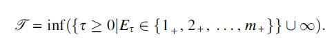
If the path length from the root to a tip of the tree is
Otherwise, at the tip that arose from reaching state
Go to Step 2.
Uncolor all edges to obtain a sampled tree.
An example simulation of a colored tree from a binary-type model is shown in Figure 1, with the color indicating type hidden in Figure 2.
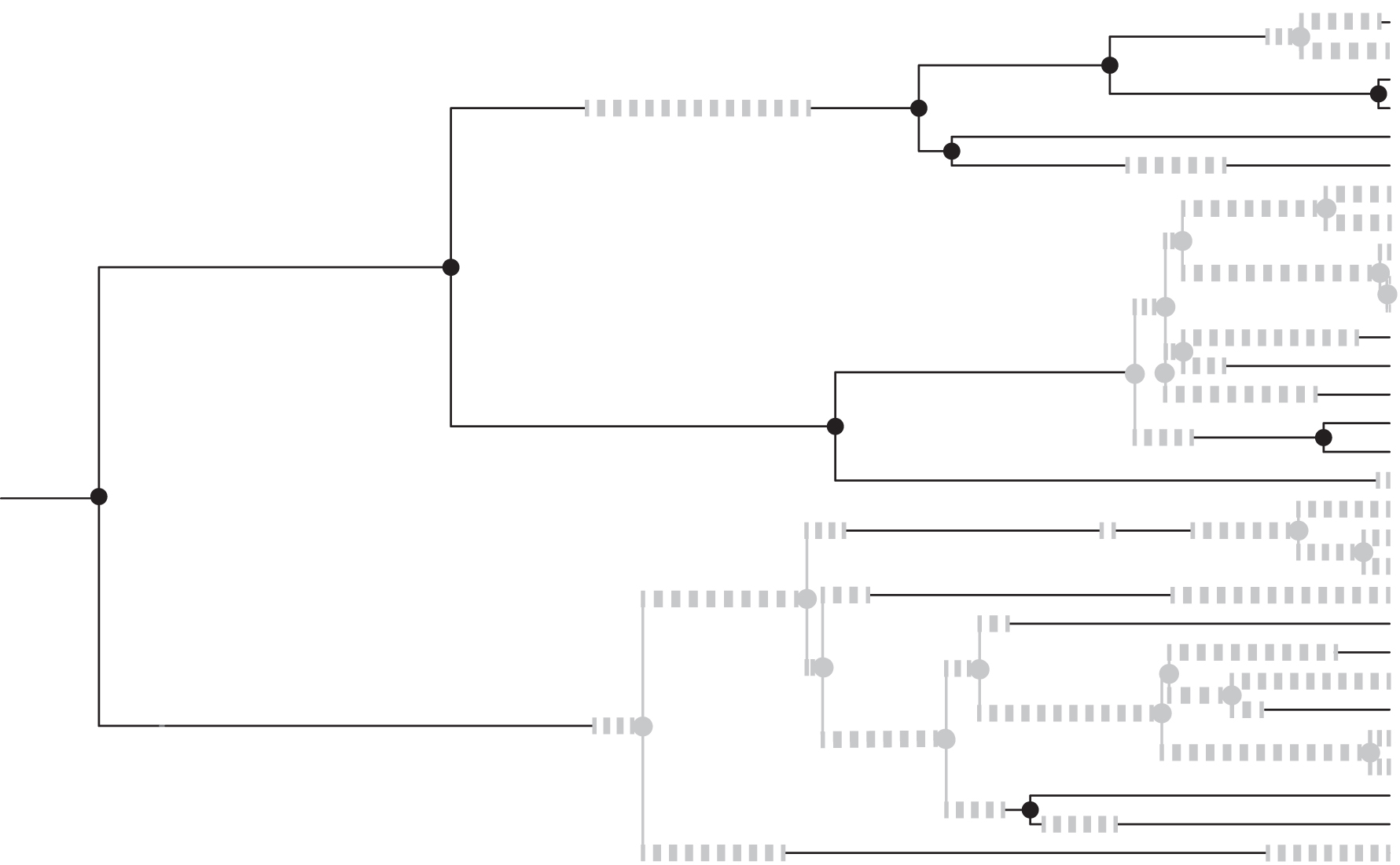
A finite-length colored tree generated by the binary-type pure birth tree model, before colors are hidden. Here black represents type 1 and dashed gray type 2, with

The uncolored tree of Figure 1, of depth T, generated by the binary-type pure birth tree model. The black line at t determines several highlighted triples of edges whose lengths are possible draws from the probability distribution GT,t of Definition 5 of Section 5.
Remark. Inherent in the model are several notions of time. For an individual edge process,

We can thus view a random tree as growing with time t, as its terminal edges lengthen while changing type, and speciate.
Remark. While we have defined the MPBT model as starting with a single edge descending from the root node, it is equally common to define diversification models as starting at a bifurcating root. The modifications to the definition that are necessary to do so are straightforward, and working in that context would have no substantive impact on the arguments which follow.
Remark. Even if
For parameters
where
Proof. For
so

For technical reasons we impose the following assumption, which is also biologically plausible.
Proof. The assumption implies that U is strictly diagonally dominant, that is, the absolute value of each diagonal entry is strictly greater than the sum of the absolute values of all other entries in its row. Thus U is nonsingular (Horn and Johnson, 2012). Since the diagonal entries are also negative, by the Gershgorin Circle Theorem every eigenvalue of U will have negative real part.
Moreover, under Assumption 1,
Proof. Since
Under Assumption 1, by Lemma 2 the eigenvalues of U have negative real parts, so
Proof. The matrix
using that U is nonsingular by Lemma 2. But

TYPE COUNTING PROCESS
Another ingredient of our approach to establishing the identifiability of MPBT model parameters is an analysis of an associated classical branching process, in which only the type counts are observed. More specifically, it records the number of edges of the tree which have each type as a function of time, but retains no information on the topology of the tree. We call this the type counting process and in this section use established results to determine the asymptotic behavior of the relative frequencies of each type.
 -valued continuous-time stochastic process over
The asymptotics of the relative frequencies follow from results of Athreya (1968) on multitype continuous-time Markov branching processes, specifically Theorems 1 and 2 of that work, which are paraphrased below as Theorem 1. Such a model can be described as a process where individuals of type i live an exponentially-distributed length of time (whose rate only depends on type) and on death may be replaced by individuals of any type according to a distribution over 
To place the type counting process of the MPBT model into this framework, both speciation and change in type are viewed as deaths. Speciation results in replacement by two individuals of the same type, and change in type results in replacement by an individual of a different type. Since a speciation “death” of a type i individual occurs with rate
and a change to type j with probability
Basic properties of the type counting process are summarized in the following.
We introduce yet another matrix defined in terms of the MPBT model parameters, as its leading eigenvalue and corresponding eigenvector play a large role in the counting process's behavior.
A leading eigenvalue of A is an eigenvalue,
The matrix A is the infinitesimal generator of the conditional expectation of the Nis. More precisely,
with
where
We will shortly show that
1. 2. A has a unique leading eigenvalue
Proof. Fix
The Perron–Frobenius Theorem applied to B shows that it has a unique dominant (i.e., of maximal absolute value) eigenvalue which is also positive and simple, with a unique normalized left eigenvector
Key properties of the counting process follow from the following more general theorem on classical branching processes.
 Let
Let
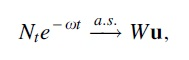
If
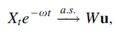
where W is a nonnegative random variable,
Moreover, if
for all

where u is the positive normalized leading left eigenvector of A.
Proof. Using the assumptions and Lemmas 3 and 4, the hypotheses of Theorem 1 are met, including inequality [Eq. (1)]. Thus
where
Since the random variable
Thus we find

for each i.
Remark. In studying diversification models with a single type but time-dependent rates of speciation and extinction, it is common to consider the random function giving the number of lineages through time in a tree. This loses no information on parameters from the full tree, as each change in its value (speciation or extinction) is equally likely to have occurred on any lineage, and the growth of this function is thus highly informative on parameter values. For the multitype pure-birth model, however, the function
Using the distributions of edge lengths and relative frequencies of each type of edge in a tree at a given time found in Sections 3 and 4, we are ready to establish identifiability of the MPBT parameters. To do so, we consider an asymptotic joint distribution of the lengths of 3 edges around a common node in the tree (Fig. 2). We seek to show that from this distribution the model parameters
Due to the conditional independence of the lengths of three edges sharing a common node, given that node's type, this distribution is a mixture of product distributions, with the mixing distribution and the components of the products closely related to distributions previously computed. This structure allows for the application of the following theorem, to obtain unmixed distributions of edge lengths conditioned on the type of the parental node. Thus, even though we have no observation of type at any point in the tree, we can extract a distribution that is conditioned on type.
The following is a variant of Theorem 8 of Allman et al (2009), with the hypotheses modified as discussed on p. 3116 of that article.
be a product of 3 independent, absolutely continuous distributions
Then, up to label swapping in i, the
More precisely, P determines distributions
To apply this theorem, we make a further technical assumption, denoting the vector of 1s by
is nonsingular.
While the role of this assumption in our arguments will be clear in our proofs of Lemma 6 and Theorem 3 below, to understand its implications concretely, consider first the case
so
The nonsingularity of M thus is equivalent to
For general m, Assumption 3 is equivalent to the nonvanishing of
The nonvanishing of
For instance, when
Nonvanishing of the polynomial, then, requires that the three
Next, we define the joint edge length distribution for several edges of a tree.
We call
The three edge lengths used in the definition of
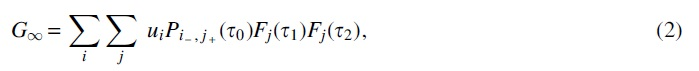
where Fj,
Proof. Note that the event E which is conditioned upon in the definition of
where the function
Letting Ai denote the event that the uniformly at random chosen edge is of type i at time

In this last expression, the only dependence on T is in
Remark. While the specific time
This immediately gives that

where
To apply Theorem 2 to
We now introduce an additional assumption, which holds for generic parameters.
Proof. Since  we need to only consider the cases
Consider first the case
Suppose
For
From Lemma 1 the vector G of all
Suppose  for some vector
  it follows that
In particular, for
To show that every pair of the
Using
We now arrive at our main result.
Proof. Suppose two parameter choices,
By Theorem 2. Corollary 2, and Lemma 6 the distributions
Using Proposition 1 the equations
where

Using Equation (4) and the definition of
Equation (4) further implies
Using Equation (5) then yields
and since M is nonsingular,
Since
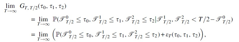
Remark. Theorem 3 establishes that an asymptotic distribution, as tree depth
Fortunately, a minor modification to the proofs above again yields identifiability of parameters from an asymptotic distribution derived from a single observation, as the depth of the tree goes to infinity. Indeed, modify Definition 5 so that GT,t is the distribution of edge lengths around a node from a single growing tree. The proof of Lemma 5, then, is modified only in its last line, as
Theorem 3 and the succeeding remark show that parameters
For applications, it would be highly desirable to extend our identifiability result to a model incorporating constant extinction rates for each type. In most biological settings, the obtainable “data,” however, is not the tree with edges stopping at extinction events, but rather the pruned tree in which all edges with no extant descendants are removed.
For a single type, parameter identifiability of a model with pruning was essentially considered by Nee et al (1994), where it was shown that the lineages-through-time function's rate of change allowed the speciation and extinction rates to be determined, by separately considering the time regimes much earlier than the tree tips and near the tree tips. An analysis combining the insight from Nee et al (1994) with the mixture distribution framework used in this work might be successful in showing that parameters can be recovered from a single large tree observation for the multitype birth–death tree model.
We emphasize that our work here in no way suggests that a multitype model incorporating arbitrary time-dependence in its rates will have identifiable parameters. Indeed, the issues that Louca and Pennell (2020) raised are likely to only be compounded in such a setting, unless the time-dependence is restricted to some specific form. Results such as those of Legried and Terhorst (2022a, 2022b) in the single-type case, which show identifiability for piecewise constant and polynomial time-dependent rates, can be expected to generalize to more types.
Another interesting identifiability question for multitype tree models concerns what information on parameters is contained in the tree topology alone or from weaker metric information than precise branch lengths. While our analysis depends heavily on metric features of the tree, that of Popovic and Rivas (2016) required no metric information. However, it did use type observations at the tips of the tree and at their parental nodes. While types at tree tips may be observed in some biological studies, types of the parental nodes are generally not observable, as data are generally collected only from the taxa extant at the present. Even if ancient DNA or other trait data from earlier times are available, it is unlikely to be from the time of the last speciation.
Footnotes
AUTHORs' CONTRIBUTIONS
All authors contributed equally to this work.
AUTHOR DISCLOSURE STATEMENT
The authors declare they have no competing financial interests.
FUNDING INFORMATION
E.S.A. and J.A.R. were supported, in part, by NSF Grant DMS-2051760.