Gene Regulatory Network Inference Using Convolutional Neural Networks from scRNA-seq Data

Abstract

In recent years, with the rapid development of single-cell sequencing technology, this brings new opportunities and challenges to reconstruct gene regulatory networks. On the one hand, scRNA-seq data reveal statistical information of gene expression at single-cell resolution, which is beneficial to construct gene expression regulatory networks. On the other hand, the noise and dropout of single-cell data bring great difficulties to the analysis of scRNA-seq data, resulting in lower accuracy of gene regulatory networks reconstructed by traditional methods. In this article, we propose a novel supervised convolutional neural network (CNNSE), which can extract gene expression information from 2D co-expression matrices of gene doublets and identify interactions between genes. Our method can avoid the loss of extreme point interference by constructing a 2D co-expression matrix of gene pairs and significantly improve the regulation precision between gene pairs. And the CNNSE model is able to obtain detailed and high-level semantic information from the 2D co-expression matrix. Our method achieves satisfactory results on simulated data [accuracy (ACC): 0.712, F1: 0.724]. On two real scRNA-seq datasets, our method exhibits higher stability and accuracy in inference tasks compared with other existing gene regulatory network inference algorithms.

1. INTRODUCTION

Gene regulatory network (GRN) consists of transcription factors, genes, and regulatory systems. Each node of the GRN represents a TF or a gene. Edges connecting transcription factors (TFs) to target genes represent regulation. Edges are labeled as either activated or repressed, showing the regulatory function of transcription factors on their target genes (Mao et al, 2022; Marbach et al, 2012). The GRNs underlie cellular identity and primary function in most biological processes and complex diseases (Hamey et al, 2017).

Due to the difficulty of large-scale gene regulatory network exploration experiments, computational network inference methods have been widely used to infer gene regulatory networks. Given the complexity of GRNs, for example, even seemingly homogeneous populations of cells may exhibit significant transcriptional variation (Landan et al, 2012). Thus, single-cell analysis becomes feasible. scRNA-seq data provide a two-dimensional matrix of cells and genes, with each value representing the expression level of the gene in the cell. However, scRNA-seq data have features such as low signal-to-noise ratio and high sparsity, which are caused by measurements, which bring great challenges to the analysis of scRNA-seq data (Aubin-Frankowski and Vert, 2020).

In recent years, with the popularity of scRNA sequencing technology, many approaches have been proposed for reconstructing gene regulatory networks from different computational perspectives. It is roughly divided into the following four types: (1)

Regression-based methods. The regression method is that the expression level of one gene is determined by the regression coefficients of the expression levels of several other genes. Such classic representative methods are GENIE3 (Va et al, 2010). The GENIE3 method employs random forests and extra trees to solve regression problems. An obvious disadvantage of this type of approach is that complex nonlinear regulatory relationships cannot be found

(2)

Ordinary differential equation-based (ODE) method. The ODE approach describes the gene regulatory network as a complex dynamical system. The S-system model (Nakayama et al, 2011) is one of the nonlinear differential equation models of gene regulatory networks, which can describe various dynamics of relationships between genes. Such methods are limited by the computational speed and insufficient data volume, and they can only be applied to some simple control networks.

(3)

Gene co-expression analysis-based method. Gene co-expression analysis usually uses Pearson correlation or mutual information (Song et al, 2012) methods. The relationship between genes obtained with this type is symmetric, which means that there is only one relationship value per pair. This is advantageous for some applications (e.g., clustering), but it is problematic for network reconstruction tasks because the direction of regulation between each pair of genes cannot be clearly defined.

Several research methods have been proposed to address the regulatory direction problem, such as SINGE (Deshpande et al, 2022), LEAP (Specht and Li, 2016), and SCRIBE (Qiu et al, 2018). SINGE (Deshpande et al, 2022) uses Granger causality to detect correlations in single-cell gene expression data annotated with pseudo-times. An obvious drawback of this method is that the association between pseudo-time trajectories and cellular sorting cannot be verified. LEAP (Specht and Li, 2016) utilizes the estimated pseudotime of the cells to find gene co-expression that involves time delay.

This method is able to infer direct associations between genes and cannot identify indirect associations between genes. SCRIBE (Qiu et al, 2018) employs Restricted Directed Information to determine causality by estimating the strength of information transferred from a potential regulator to its downstream target. This method is only suitable for small-scale gene regulatory networks. For complex and large-scale gene networks, SCRIBE (Qiu et al, 2018) has difficulty in predicting accuracy fairly quickly.

(4)

Deep learning-based methods. Some methods based on deep learning have been proposed for designed a deep learning framework to integrate known gene interactions and gene expression data for predicting and discovering new interactions.

Yuan et al (2019) used convolutional neural networks (CNN) to infer GRN, named CNNC. They converted the expression data of TF and target gene into a two-dimensional matrix by calculating the 2D histogram. Then, they normalized it as the input of CNN and achieved good results. Chen et al (2021) proposed a new supervised deep neural network called DeepDRIM, which represents the joint gene expression distribution of gene pairs as images. The neural network uses the image of target TF-gene pairs and the image of potential neighbors for dichotomization.

Due to the consideration of the neighborhood environment of TF-gene pairs, DeepDRIM (Chen et al, 2021) can effectively eliminate false positives caused by transmitted gene-gene interactions. However, the DeepDRIM method adds the neighbor images of genes, making the algorithm's running time and memory quite large. Zhao et al (2022) developed a hybrid deep learning framework DGRNS, which includes a gated recursive unit network for exploring time-related information and a CNN for learning spatial-related information.

It uses sliding windows to extract valuable features while maintaining the direction of adjustment. The DGRNS method (Zhao et al, 2022) is using a sliding window to extract features, which also results in the loss of useful information. A complex neural network structure is used, which leads to quite large training parameters. In the previous method, Li et al (2022) added image data to predict the regulation between gene pairs by using CNN (SDINet) method to fuse gene expression images and histogram between genes in RNA-seq data for image classification. Although the CNNC method and the SDINet method have good performance compared with other non-deep learning methods, they suffer from histogram distortion caused by dropouts and extreme values.

Due to the high noise and dropouts of scRNA-seq data, we propose a new deep convolutional network model (supervised convolutional neural network [CNNSE]) with better performance, which uses 2D CNN to classify 2D co-expression matrices of gene doublets to predict regulatory relationships. Our method can avoid the loss of extreme point interference by constructing a 2D co-expression matrix of gene pairs. Further, most CNN-based methods mainly focus on extracting high-level semantic information of images, while ignoring detailed information.

This is because the convolutional network model (CNN) applies multiple downsampling to obtain a larger receptive field, resulting in reduced resolution of the feature maps. To solve the problems cited earlier, the CNNSE model designs two branches for image data. One branch acquires high-level semantic information, and the other branch preserves detailed information using spatial pyramid pooling (Chen et al, 2017) and channel attention mechanism, specifically as shown in Figure 2. Our model is trained and tested on the BEELINE dataset: BEELINE is an evaluation framework for benchmarking different GRN inference algorithms based on single-cell transcriptome data.

Experiments show that our model achieves satisfactory results on simulated data [accuracy (ACC): 0.712, F1: 0.724]. On two real scRNA-seq datasets, our method exhibits higher stability and accuracy in inference tasks compared with other existing GRN inference algorithms.

2. METHODS

The entire flow chart of our CNNSE algorithm is shown in Figure 1, which is divided into data preprocessing, building a 2D co-expression matrix, and a deep CNN model.

FIG. 1.

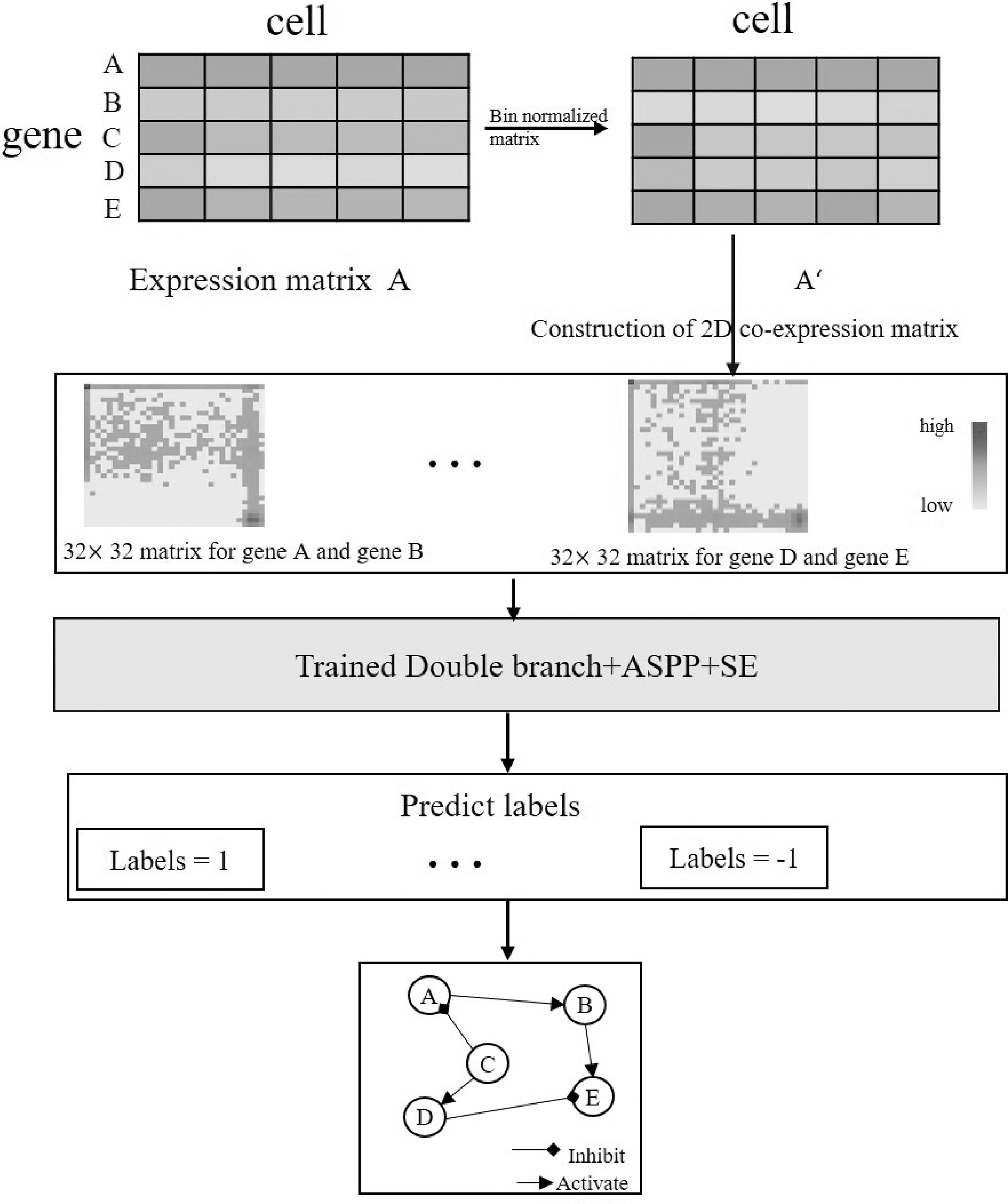
The whole GRN inference process. GRN, gene regulatory network.

2.1. Problem statement

In this study, we aim at predicting the regulatory interactions between TFs and target genes according to the features extracted from their expression level. Thus, the input is a pair of genes, and the output label is 0 or 1, denoting the existence of the regulatory relationship, that is, a binary classification problem. scRNA-seq provides a sparse gene expression matrix with g rows and c columns. $A^{g \times c} = [\begin{matrix} a_{11} & \dots & a_{1 c} \\ \dots & \dots & \dots \\ a_{g 1} & \dots & a_{g c} \end{matrix}]$ (1)

where g is the number of genes and c is the number of cells. $a_{i j}$ is the expression value of the ith gene in the jth cell. Let G be the set of genes and R the set of unknown regulatory edges. Reconstructing a GRN is to build a directed network $(G, R)$ from scRNA-seq expression data.

2.2. Construction of 2D co-expression matrix

A 2D co-expression matrix $E_{x y}$ reflects the co-expression distribution of x and y genes in all cells. Here, we set the matrix size to $32 \times 32$ , which is determined according to the appropriate amount of accurately retaining information and consuming disk space. For each gene, we first discretize the expression value of the gene into integers 1–32. This has the disadvantage that extreme points stretch the entire range, causing normal points to squeeze together instead of being uniformly distributed across all bins. The solution is to reduce the extreme points by reducing the variation of gene expression values.

The zero elements in the gene expression matrix are mainly caused by dropouts, and we label the zero elements as NaN. The extreme points still exist after the logarithm of all non-zero elements, so the bins of each gene need to be calculated in a limited range. The specific operations are as follows:

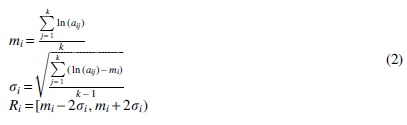
where k is the number of non-zero elements in the expression value of the ith gene, m_i is the mean of the non-NaN values of the ith gene, $σ_{i}$ is the standard deviation of the non-NaN values for the ith gene, and R_i is the range of the ith gene. Then, we divide R_i into 32 bins of equal range: $R_{i k} = [m_{i} + \frac{(k - 17) σ_{i}}{8}, m_{i} + \frac{(k - 16) σ_{i}}{8}), k = 1, 2, \dots, 32 .$ (3)

Discretizing all genes, we can rewrite the expression values as their bin index numbers and obtain the bin-normalized matrix B: $B^{g \times c} = [\begin{matrix} b_{11} & \dots & b_{1 c} \\ \dots & \dots & \dots \\ b_{g 1} & \dots & b_{g c} \end{matrix}]$ (4) $b_{i j} = \{\begin{matrix} k, ln (a_{i j}) \in R_{i k} \\ 1, ln (a_{i j}) < m_{i} - 2 σ_{i} o r a_{i j} = N a N . \\ 32, ln (a_{i j}) \geq m_{i} + 2 σ_{i} \end{matrix}$ (5)

Here, $b_{i j}$ is the integer expression level of the ith gene in the jth cell. Based on the bin normalization matrix B, we can construct a co-expression matrix for all gene pairs. The specific algorithm flow is in Algorithm 1. Specifically, we first set the element in the co-expression matrix E to 0, and then scan each column in matrix B in turn to obtain two integer values of gene x and gene y in each cell. We use the two integers as index to find the element in E, and plus it by 1 to record one co-expression of the two genes.

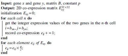
Then, we multiply each element by a factor such that the sum of all elements in the 2D matrix is a constant p. We set p to 4096 in our experiments. The time complexity of constructing the 2D co-expression matrix is $O (g c) + O (c)$ .

Algorithm 1: The co-expression matrix of the two genes.

2.3. CNNSE model

Our task is to judge whether there is an interaction between genes, so we treat it as an image classification problem. For single-cell gene expression data, we used the 2D co-expression matrix as the input to the CNNSE model to calculate the interaction probability between genes. We propose a CNNSE model for analyzing gene co-expression matrix data based on ResNet18 (He et al, 2016).

To reduce overfitting, we halve the number of convolution kernels in each layer of ResNet18. We describe our modified ResNet18 next and show it in Figure 2. We add a multi-scale detail branch that does not perform downsampling based on our modified ResNet18. Not performing downsampling preserves more information, but it reduces the receptive field. Therefore, we introduce the atrous spatial pyramid pooling (ASPP) module (Ayanzadeh, 2019). The schematic diagram of the model is shown in Figure 3.

FIG. 2.

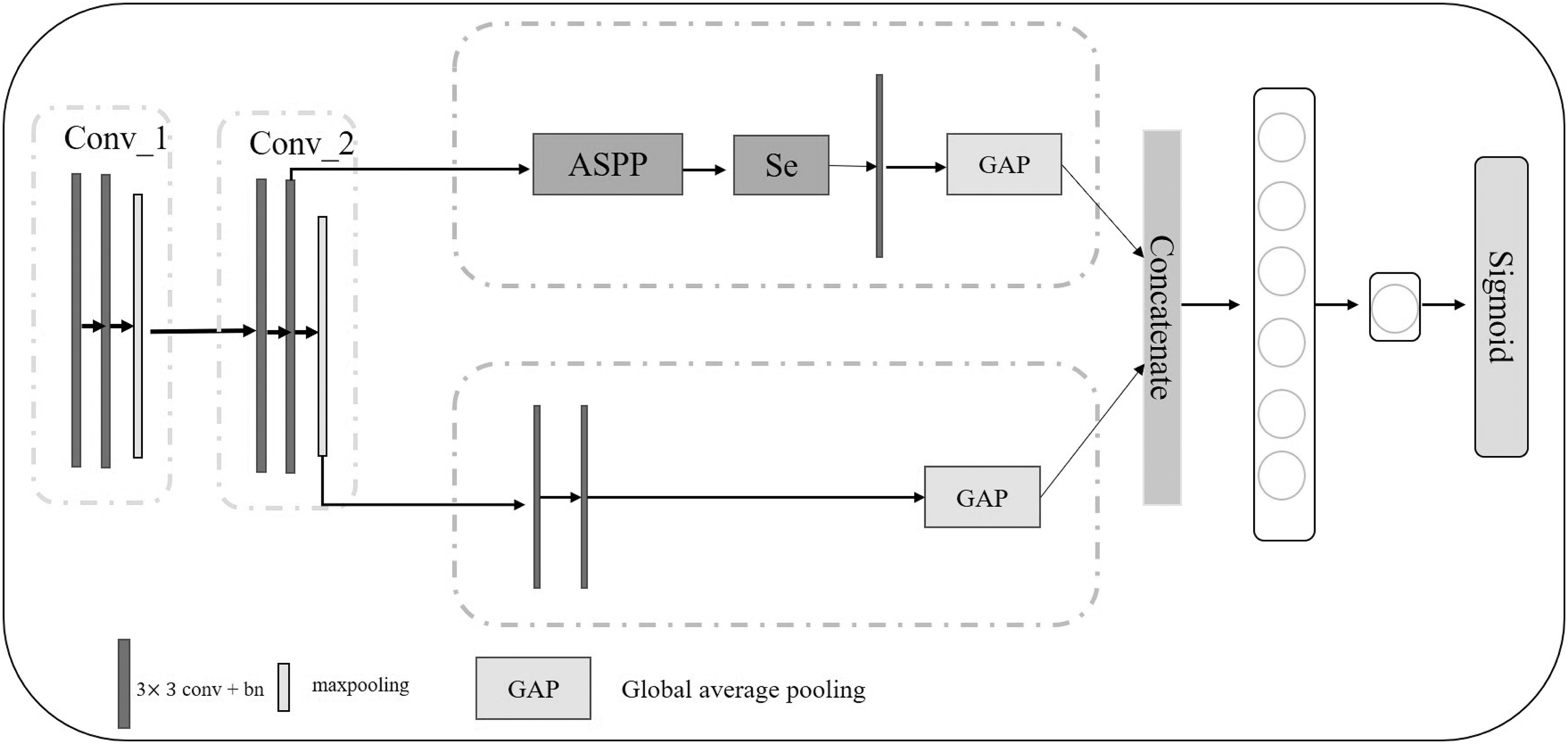
The structure of CNNSE model. It applies ResNet18 as the backbone. It contains the multi-scale detail branch and high-level semantic branch, which extract multi-scale information and high-level semantic information, respectively. CNNSE, supervised convolutional neural network.

FIG. 3.

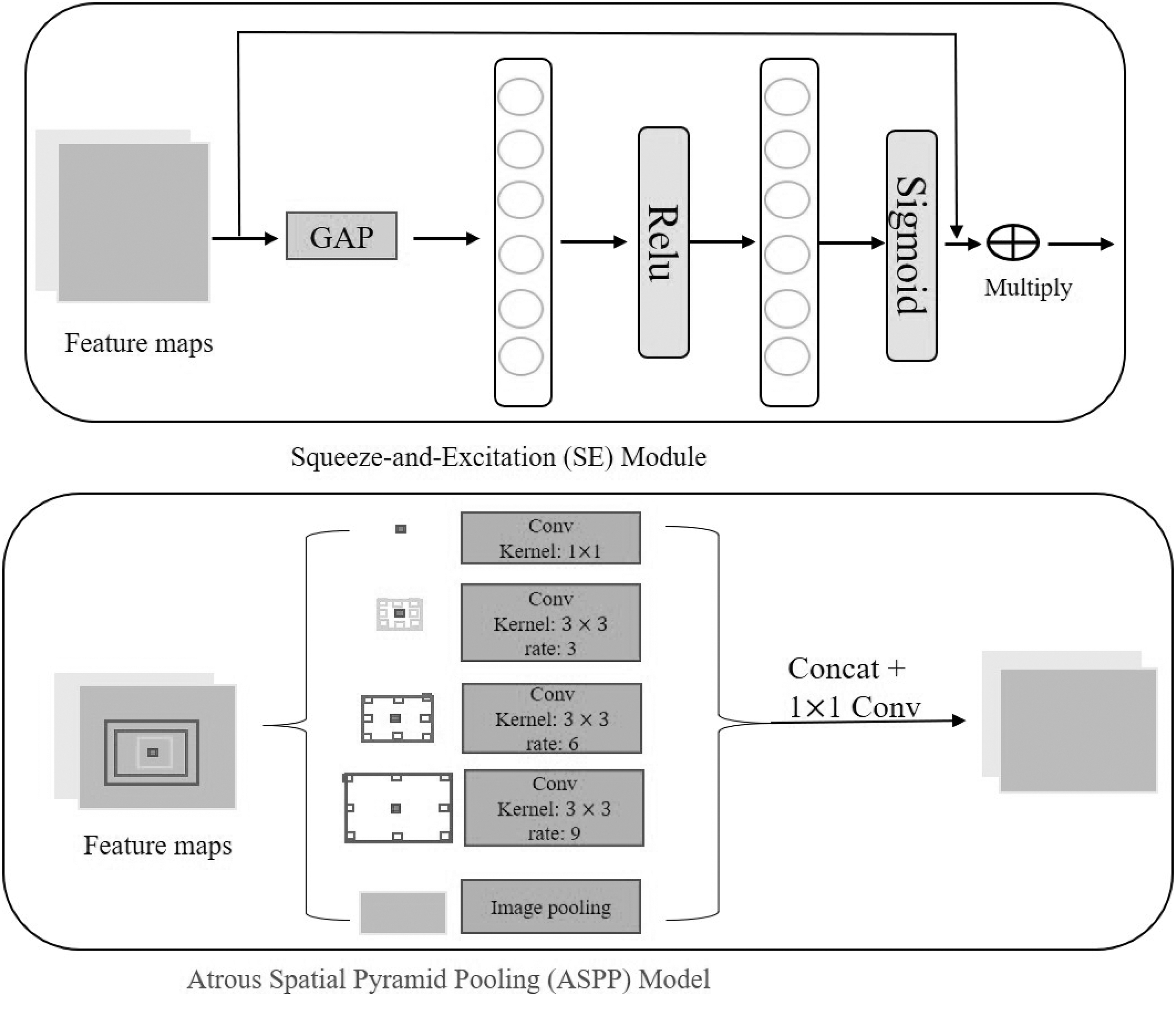
The structure of SE module and ASPP module. The SE module uses two fully connected layers to learn the relationships among channels and recalibrate the channels. The ASPP module applies detailed convolutions at different rates to obtain the information of different scales. ASPP, atrous spatial pyramid pooling; SE, squeeze-and-excitation.

This module applies dilated convolutions at different rates to obtain receptive fields of different scales and semantic information. In other words, we apply ASPP instead of downsampling to obtain multi-scale detail information, which is beneficial to extract objects of different sizes. The ASPP concatenates all feature maps of different scales, which may add redundant information. Therefore, we add the squeeze-and-excitation (SE) module (Hu et al, 2017) (shown in Fig. 3) after ASPP to learn the relationship between channels and recalibrate the channels.

Finally, the semantic branch and the multi-scale detail branch are combined for final prediction. The two branches can obtain complementary information, which greatly improves the prediction performance. The CNNSE model adds a multi-scale detail branch after Conv_2, as shown in Figure 2. This is because adding branches too early extracts more redundant information.

2.3.1. ASPP model

As shown in the lower panel in Figure 3, the ASPP module uses dilated convolutions at different rates to obtain different receptive fields. Further, ASPP uses image pooling to obtain global features. Finally, these features are concatenated, and then the feature channel is reduced by $1 \times 1$ convolution. The formula can be expressed as follows: $Z = f_{1}^{1} (f_{1}^{1} (x) ⨁ f_{3}^{3} (x) ⨁ f_{3}^{6} (x) ⨁ f_{3}^{9} (x) ⨁ U (a v e (x)))$ (6)

where $f_{m}^{n}$ represents the convolution kernel size is m, the rate is n, $⨁$ is the connection operation, ave is the averaging operation, and U represents the upsampling by linear interpolation. The ASPP module obtains receptive fields at different scales while maintaining the resolution of feature maps.

2.3.2. SE module

The previous step ASPP concatenates all features at different scales, but not all features are useful. Therefore, a channel attention mechanism is added after ASPP to filter out useless features. We directly apply the SE block (Hu et al, 2017) to weight the channel features. As shown in the upper graph in Figure 3, in SE, the channel features are constructed by two fully connected layers, and then the channel weights are output by the sigmoid layer. The channel weights are then multiplied by the original features. The formula can be expressed as follows:

where x is the input feature, and W and H are the width and height of the feature map, respectively. represents global average pooling, f is a fully connected layer, and $⨁$ represents element-wise multiplication.

3. RESULTS

To conduct a comprehensive and detailed evaluation of CNNSE, we analyzed the importance of each module of the deep learning framework, the effectiveness of the method framework, and the accuracy of the results. Through a series of comparative experiments with different model frameworks, it is shown that the deep learning framework in CNNSE is reasonable and applicable. By comparing with the latest methods, CNNSE is proved to outperform other state-of-the-art approaches. In addition, the robustness, accuracy, and stability of CNNSE are proved by applying our model to datasets of different tissues.

3.1. Experimental data

We use the dataset under the BEELINE framework (Pratapa et al, 2020) for experiments. One simulated data and two scRNA-seq datasets were selected for testing the performance of the CNNSE model and the other four algorithms. The in silico dataset was created by randomly simulating hematopoietic stem cell (HSC) differentiated GRNs using the BoolODE (Pratapa et al, 2020) model. The number of genes in HSC is 11, the number of simulated cells is 2000, and pseudo-time information is provided.

Mouse embryonic stem cells (mESCs)(Hayashi et al, 2018) and erythroid mouse hematopoietic stem cells (mHSC-E)(Nestorowa et al, 2016) are two scRNA-seq datasets. mHSC-E contains 4764 genes and 1071 cells, and its GRN is constructed from the ChIP-Atlas database. The mESCs contain 18,387 genes and 421 cells, of which ESCAPE and ChIP-Atlas are GRN sources.

3.2. Experimental setup

Positive samples are composed of TF–Target gene pairs whose directed regulatory relationship is recorded in the standard network. Negative samples are TF–gene pairs that are not included in the standard network. Since the sparsity nature of in vivo GRNs, the number of negative samples is much larger than that of positive samples. All TF-gene pairs with regulatory relationships were first divided into training and test sets in a ratio of 8:2.

The number of negative samples in the training set is determined by the number of positive samples, that is, by the ratio of positive samples to negative samples. We use Adam as the optimizer, and the initial learning rate is set to $3 e^{- 4}$ . We use 1, −1, 0 to denote activation, inhibition, and no regulation. Therefore, our task is to use the CNNSE model for classification predictions of the 2D co-expression matrix. We use conventional accuracy, F1 score, AUC, and AUPR as our evaluation metrics.

Among them, the F1 score takes into account the precision and recall of the classification model. AUC is the area under the ROC curve. AUPR is the area under the precision-recall curve. The larger their values, the better the model performance.

3.3. Ablation experiment for CNNSE

To verify the effectiveness of the multi-scale detail branch, our CNNSE model applies ablation experiments on the HSC dataset, as shown in Table 1. A single branch represents our backbone, which is our modified ResNet18. A double branch means that we add a new branch to the trunk. Their detailed model architectures are shown in Figure 4. The accuracy of Double branch and Single branch+ASPP+SE reach 0.533 and 0.571, respectively, which are better than that of Single branch.

FIG. 4.

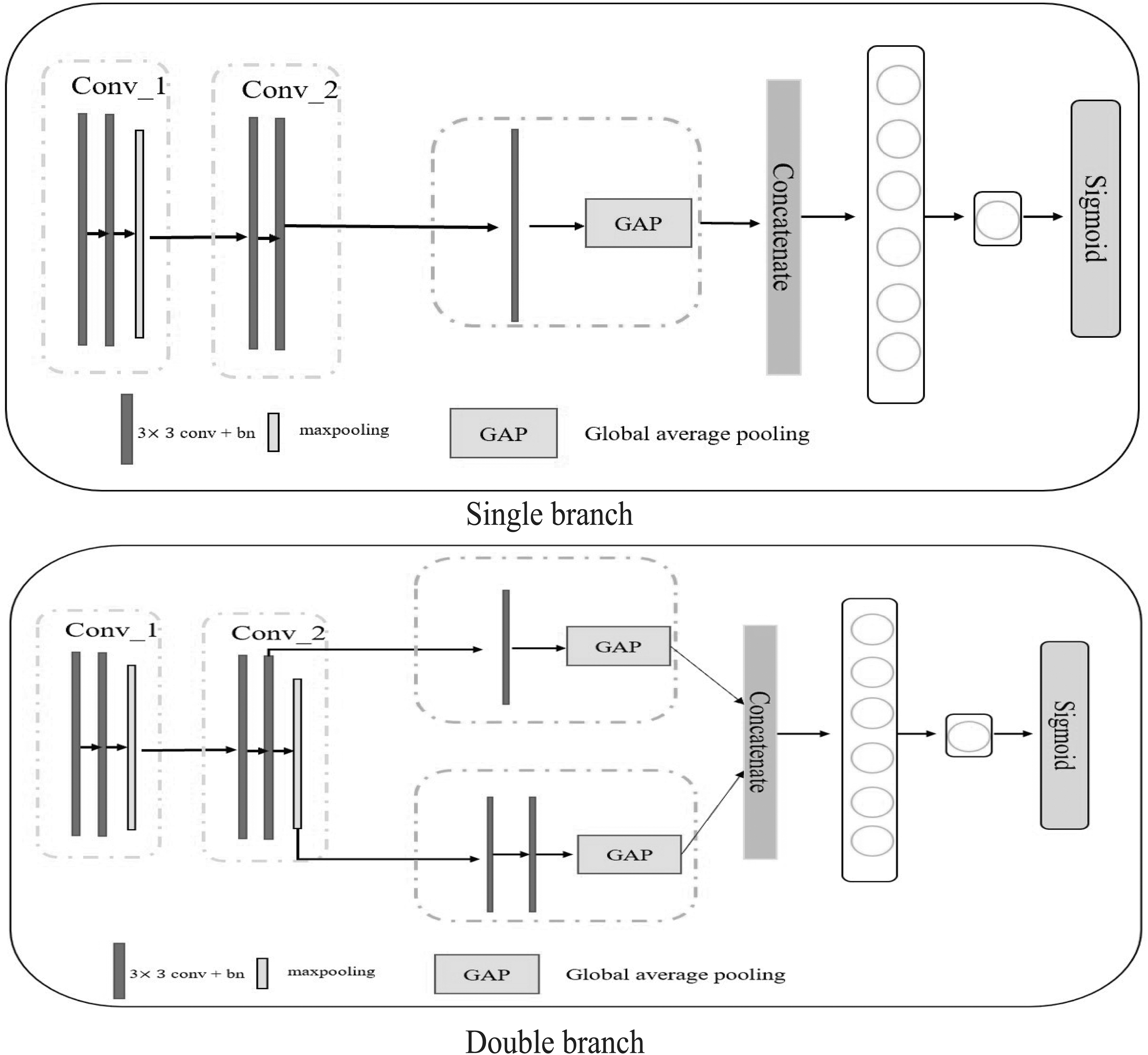
The structure of single branch module and double branch module.

Table 1.

Ablation Experiment for Supervised Convolutional Neural Network

Model	ACC	F1
Single branch	0.524	0.518
Single branch+ASPP+SE	0.571	0.589
Double branch	0.533	0.557
Double branch+ASPP	0.594	0.601
Double branch+SE	0.606	0.615
Double branch+ASPP+SE	0.712	0.724

Bold font indicates maximum value.

ACC, accuracy; ASPP, atrous spatial pyramid pooling; SE, squeeze-and-excitation.

It shows that one branch extracts potential high-level semantic features between genes, and the other branch extracts multi-scale details of gene pair co-expression matrix. The role of these two branches extracts the importance features of gene co-expression matrix sufficiently to better reflect the intensity of gene correlation. Double+ASPP does not outperform Double+ASPP+SE, which means that multi-scale detail information is not all useful.

Among them, the Single branch has the worst performance with an accuracy rate of 0.524, which shows that useless and redundant details can even have a bad impact on our model. In short, high-level semantics and multi-scale detail information are very important, but not all scale features are useful. Therefore, SE is also very important for filtering multi-scale information.

Because of the randomness of the neural network, the results will change for each run. In fact, these methods are run 10 times. The area under the receiver operating characteristic curve (AUROC) and AUPR are shown in Figures 5 and 6 respectively. As shown in Figure 5, the results of 10 run of our method are stable, and the average value of our method is better than that of other methods, which further illustrates the effectiveness and robustness of our method.

FIG. 5.

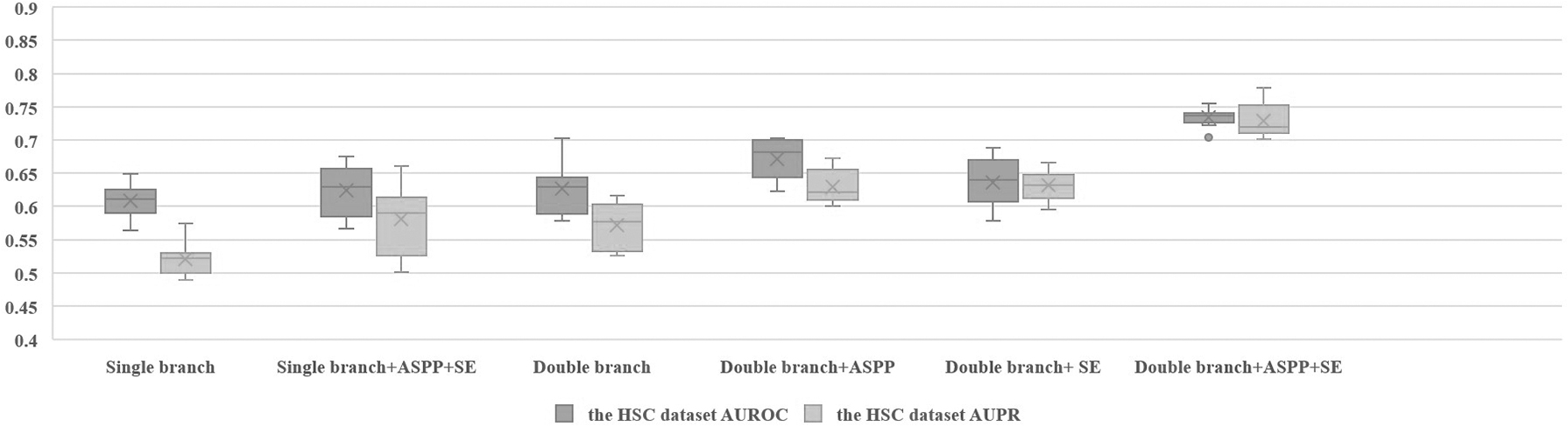
The AUROC and AUPR of the different model architectures on the HSC dataset. AUPR, area under precision-recall curve; AUROC, area under the receiver operating characteristic curve; HSC, hematopoietic stem cell.

FIG. 6.

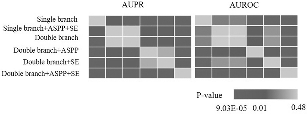
Mann–Whitney test for six AUROC and AUPR distributions on the HSC dataset.

The significant differences between the AUROC and AUPR distributions of different structures are analyzed in Figure 5, and the Kruskal–Wallis test is performed on the six structures to obtain p-values of $2.03 e^{- 06}$ and $9.07 e^{- 09}$ for the AUROC and AUPR distributions, respectively, both of which are less than 0.01. The test reports a statistically significant difference; they perform pairwise tests such as the Mann–Whitney test.

The results are shown in Figure 6. Double branch+ASPP+SE is significantly different from all the other five structures of the method. It further proves that the structure of our method is significantly effective. It can provide an effective research tool for reconstructing GRNs.

3.4. Comparison of model architectures

To verify the validity of 2D co-expression matrix and convolutional neural module constructed by our method respectively, we will construct the following models to compare with our model: The first is the CNNC method; the second is the 2D histogram constructed by the CNNSE method and the deep learning model of the CNNC method, which is called a variation of the CNNC method (CNNC_var); the third is the 2D histogram constructed by the CNNC method and the deep learning model of the CNNSE method, which is called a variation of the CNNSE method (CNNSE_var); and the fourth is our CNNSE model. To verify the effectiveness of each module, we conducted verification on two real scRNA-seq datasets: mESCs dataset (Hayashi et al, 2018) and mHSC-E.

Since raw datasets are usually massive and redundant, preprocessing is essential to screen out genes that contain valuable biological information. By calculating the variance and P value of each gene expression vector, we only focus on those genes whose P value is lower than 0.01. To evaluate the effectiveness of the module, we rank all genes in descending order of variance, and we take the first 200 genes to form a dataset. The performance results of four different model frameworks run 10 times on these two datasets are shown in Figure 7.

FIG. 7.

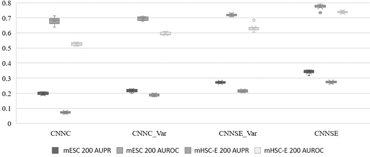
Performance of different model architectures.

As shown in the figure, comparing the results of the CNNC method and the CNNC_Var model on these two datasets, the CNNC_Var model is obviously better than the CNNC method. This shows that our method is reliable in constructing 2D co-expression matrices, and it further verifies that our method can effectively solve the extreme point problem generated by using histograms to construct co-expression matrices.

Compared with the experimental results of the CNNC method, the CNNSE_Var model also has a significant improvement, which shows that when using the same histogram to construct the co-expression matrix, the neural network model constructed by our method to extract gene features is more important and more able to filter out useful information, and to filter out redundant information. Therefore, the experimental results show that the neural network model constructed by our method is more effective than the neural network model constructed by the CNNC method.

To further investigate the results of the different models in Figure 7, we perform statistical tests on these results. The Kruskal–Wallis test is performed on the results of the two metrics in both datasets separately, with p-values <0.01. As in the previous section, the Mann–Whitney test is then performed. The results are presented in Figure 8.

FIG. 8.

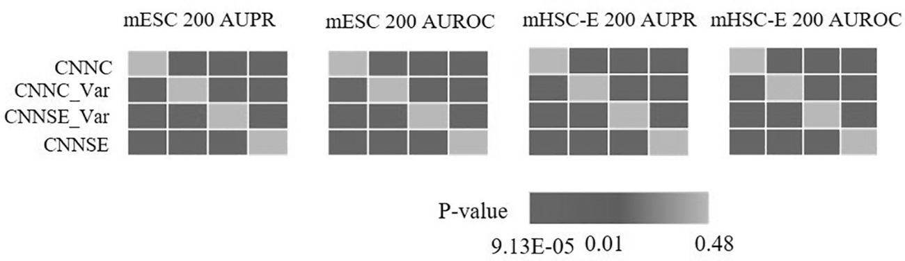
Mann–Whitney test for AUROC and AUPR distributions of different model architectures.

The significance performance of CNNSE in the figure shows that the 2D co-expression matrix and neural network model constructed by our method can accurately ignore interference information and identify significant features meanwhile, which makes a great contribution to the recognition of TF-Target regulation.

3.5. Comparison with other outstanding methods

To fully verify the performance of our proposed CNNSE model, we compare it with five classic algorithms for building GRNs in recent years, specifically CNNC (Yuan et al, 2019), 3DCEMA (Fan and Ma, 2021), DeepDRIM (Chen et al, 2021), SDINet (Li et al, 2022), and GENIE3 (Va et al, 2010). The 3DCEMA (Fan and Ma, 2021) method uses a 3D CNN to predict gene regulation by classifying a 3D co-expression matrix of gene triplets.

In the experiments, we use the same training configuration as the CNNSE model for the other four algorithms. We performed validation on two real scRNA-seq datasets: mESCs (Hayashi et al, 2018) and mHSC-E (Nestorowa et al, 2016). We choose 200, 500 genes from mESC and mHSC-E to build four datasets. In each dataset, genes are divided into two groups with no intersection: one for training and the other for testing. In the training phase, the proportions of class 0 and 1 (including +1/−1) are set to 0.8 and 0.2. During testing, the output of the last layer is used as the predicted edge weights.

The experimental results are shown in Tables 2 and 3. The algorithm outperforms all competing methods on scRNA-seq datasets (mESC and mHSC-E), including deep learning methods CNNC, DeepDRIM, 3DCEMA, and SDINet. Except on the mHSC-E 200 dataset, our model is 0.016 less than the SDINet method in AUPR value. The SDINet method uses the CNNC method to construct the co-expression histogram between genes, so it will also have an impact on the final prediction result.

Table 2.

Results on Mouse Embryonic Stem Cell Datasets

	mESC 200		mESC 500
Model	AUPR	AUROC	AUPR	AUROC
GENIE3	0.096	0.514	0.128	0.503
CNNC	0.196	0.694	0.136	0.524
DeepDRIM	0.184	0.676	0.131	0.531
3DCEMA	0.126	0.656	0.131	0.564
SDINet	0.217	0.689	0.234	0.627
CNNSE	0.351	0.785	0.314	0.759

Bold font indicates maximum value.

AUPR, area under precision-recall curve; AUROC, area under the receiver operating characteristic curve; CNNC, convolutional neural networks (CNN) to infer GRN; CNNSE, supervised convolutional neural network; mESC, mouse embryonic stem cell.

Table 3.

Results on Erythroid Mouse Hematopoietic Stem Cells Datasets

	mHSC-E 200		mHSC-E 500
Model	AUPR	AUROC	AUPR	AUROC
GENIE3	0.074	0.500	0.039	0.500
CNNC	0.077	0.534	0.145	0.651
DeepDRIM	0.164	0.662	0.184	0.691
3DCEMA	0.145	0.674	0.194	0.692
SDINet	0.217	0.761	0.264	0.721
CNNSE	0.274	0.745	0.341	0.802

Bold font indicates maximum value.

mHSC-E, erythroid mouse hematopoietic stem cells.

For CNNC, the noise will disturb the co-expressed histogram of x and y, affecting the final prediction result. By using the third dimension for comparison, 3DCEMA can avoid this interference to a certain extent, but it introduces more redundant information resulting in more false positives. Our CNNSE model constructs a 2D co-expression matrix, which avoids the interference of extreme points and also makes full use of the high-level semantic information and detailed information in the 2D co-expression matrix to predict gene interactions. Experiments demonstrate that our CNNSE model has important value in reconstructing gene regulatory networks.

4. DISCUSSION

We propose new methods and ideas to infer GRNs. We propose a deep learning method called 2D co-expression matrix, named CNNSE. CNNSE first constructs a 2D co-expression matrix of gene duplexes, and it then predicts gene regulation by classifying the 2D co-expression matrix. And the CNNSE model uses deep CNN to simultaneously extract detailed features and high-level semantic features of matrix data.

However, the properties of these two branches have no biological interpretation, and extending the models to have biological interpretability will be important in the future. Models in the dataset partitioning problem may lead to information leakage from training to testing, and future work can perform inductive evaluation like in the case of CNNC. In addition, the parameters and computational complexity of our model are small, so it is very beneficial to be applied in future experimental devices. Importantly, CNNSE outperforms other existing algorithms in both stability and accuracy, and it can serve as a reliable tool that enables researchers to more efficiently identify gene regulatory networks.

Footnotes

AUTHORs' CONTRIBUTIONS

G.M. and J.L. conceived the study, developed the methods, performed the statistical analysis, and drafted the article. Both authors have read and approved the final article. The authors agree to give consent for publication.

ACKNOWLEDGMENT

The authors thank YingTing Jiang for her helpful comments and suggestions.

AUTHOR DISCLOSURE STATEMENT

The authors declare they have no conflicting financial interests.

FUNDING INFORMATION

This research work was supported in part by the National Key Research and Development Program of China (2021YFB0300101).

References

Aubin-Frankowski

P-C

, Vert

J-P

. Gene regulation inference from single-cell RNA-seq data with linear differential equations and velocity inference. Bioinformatics, 2020; 36(18):4774–4780.

Ayanzadeh

A study review: Semantic segmentation with deep neural networks. Int J Multimed Info Retr, 2019; 7:87–93; doi: 10.1007/s13735-017-0141-z

Chen

, Cheong

, Lan

, et al. DeepDRIM: A deep neural network to reconstruct cell-type-specific gene regulatory network using single-cell RNA-seq data. Brief Bioinform, 2021; 22(6):bbab325; doi: 10.1093/bib/bbab325

Deshpande

, Chu

L-F

, Stewart

, et al. Network inference with granger causality ensembles on single-cell transcriptomics. Cell Rep, 2022; 38(6):110333; doi: 10.1016/j.celrep.2022.110333

Fan

, Ma

. Gene regulatory network inference using 3D convolutional neural network. In: Proceedings of the Conference on Artificial Intelligence (35/1);, 2021; doi: 10.1609/aaai.v35i1.16082

Hamey

, Nestorowa

, Kinston

, et al. Reconstructing blood stem cell regulatory network models from single-cell molecular profiles. Proc Natl Acad Sci, 2017; 114(23):5822–5829; doi: 10.1073/pnas.1610609114

Hayashi

, Ozaki

, Sasagawa

, et al. Single-cell full-length total rna sequencing uncovers dynamics of recursive splicing and en-hancer rnas. Nat Commun, 2018; 9:619.

, Zhang

, Ren

, et al. Deep residual learning for image recognition. In: 2016 IEEE Conference on Computer Vision and Pattern Recognition (CVPR); 2016; pp. 770–778.

, Shen

, Sun

Squeeze-and-excitation networks. CoRR abs/1709.01507, 2017. Available from: http://arxiv.org/abs/1709.01507

10.

Landan

, Cohen

, Mukamel

, et al. Epigenetic polymorphism and the stochastic formation of differentially methylated regions in normal and cancerous tissues. Nat Genet, 2012; 44:1207–1214.

11.

, Ma

, Liu

, et al. Inferring gene regulatory network via fusing gene expression image and RNA-seq data. Bioinformatics, 2022; 38(6):1716–1723.

12.

Mao

, Zeng

, Peng

, et al. Reconstructing gene regulatory of networks biological function using differential equations of multilayer perceptrons. BMC Bioinform 2022;23,, 11; doi: 10.1186/s12859-022-05055-5

13.

Marbach

, Costello

, Küffner

, et al. Wisdom of crowds for robust gene network inference. Nat Methods, 2012; 9(1548-7105):796–804.

14.

Nakayama

, Seno

, Takenaka

, et al. Inference of s-system models of gene regulatory networks using immune algorithm. J Bioinform Comput Biol, 2011; 09(supp01):75–86; doi: 10.1142/S0219720011005768

15.

Nestorowa

, Hamey

, Pijuan Sala

, et al. A single-cell resolution map of mouse hematopoietic stem and progenitor cell differentiation. Blood, 2016; 128(8):e20–e31.

16.

Pratapa

, Jalihal

, Law

, et al. Benchmarking algorithms for gene regulatory network inference from single-cell transcriptomic data. Nat Methods, 2020; 147–154.

17.

Qiu

, Rahimzamani

, Wang

, et al. Towards inferring causal gene regulatory networks from single cell expression measurements. bioRxiv, 2018; doi: 10.1101/426981

18.

Song

, Langfelder

, Horvath

, et al. Comparison of co-expression measures: Mutual information, correlation, and model based indices. BMC Bioinform, 2012; 13(1471-2105):328.

19.

Specht

, Li

. LEAP: Constructing gene co-expression networks for single-cell RNA-sequencing data using pseudotime ordering. Bioinformatics, 2016; 33(5):764–766; doi: 10.1093/bioinformatics/btw729

20.

H.-T

, A I

L W

, et al. Inferring regulatory networks from expression data using tree-based methods. PLoS One, 2010; 9(5):e12776.

21.

Yuan

, Bar-Joseph

, Horvath

, et al. Deep learning for inferring gene relationships from single-cell expression data. Proc Natl Acad Sci U S A, 2019; 116(0027-8424):27151–27158.

22.

Zhao

, He

, Tang

, et al. A hybrid deep learning framework for gene regulatory network inference from single-cell transcriptomic data. Brief Bioinform, 2022; 23(2):bbab568; doi: 10.1093/bib/bbab568