Enforcing Temporal Consistency in Migration History Inference

Abstract

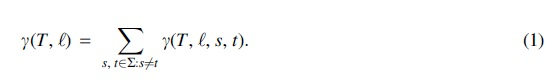
In addition to undergoing evolution, members of biological populations may also migrate between locations. Examples include the spread of tumor cells from the primary tumor to distant metastases or the spread of pathogens from one host to another. One may represent migration histories by assigning a location label to each vertex of a given phylogenetic tree such that an edge connecting vertices with distinct locations represents a migration. Some biological populations undergo comigration, a phenomenon where multiple taxa from distinct lineages simultaneously comigrate from one location to another. In this work, we show that a previous problem statement for inferring migration histories that are parsimonious in terms of migrations and comigrations may lead to temporally inconsistent solutions. To remedy this deficiency, we introduce precise definitions of temporal consistency of comigrations in a phylogenetic tree, leading to three successive problems. First, we formulate the temporally consistent comigration problem to check if a set of comigrations is temporally consistent and provide a linear time algorithm for solving this problem. Second, we formulate the parsimonious consistent comigrations (PCC) problem, which aims to find comigrations given a location labeling of a phylogenetic tree. We show that PCC is NP-hard. Third, we formulate the parsimonious consistent comigration history (PCCH) problem, which infers the migration history given a phylogenetic tree and locations of its extant vertices only. We show that PCCH is NP-hard as well. On the positive side, we propose integer linear programming models to solve the PCC and PCCH problems. We demonstrate our algorithms on simulated and real data.

1. INTRODUCTION

Studying the precise pattern of migration of biological populations holds significant importance in various areas of biology and medical science. For instance, understanding the migration history of metastatic cancer can provide insights into the mechanism of metastasis and aid in the development of novel drugs (Comen et al., 2011; El-Kebir et al., 2018; Faries et al., 2013; Sanborn et al., 2015; Somarelli et al., 2017; Tabassum and Polyak, 2015). Similarly, investigating the transmission of pathogens can help in identifying the source of an outbreak and tracing the patterns of disease spread (Campbell et al., 2019; Dellicour et al., 2018; Faye et al., 2015; Ferguson et al., 2001; Spada et al., 2004).

To successfully trace the migration history of a biological population, one may analyze genomic data as the migrated subpopulations have evolved independently, resulting in genomic differences that are location specific. More specifically, from the genomic data, one may first construct a phylogenetic tree T with each vertex v corresponding to a subpopulation with similar genetic makeup, and then label each vertex v with their location of origin $ℓ (v)$ . As such, directed edges $(u, v)$ with distinct labels at their endpoints, that is, $ℓ (u) \neq ℓ (v)$ indicate subpopulation u migrating from $ℓ (u)$ to $ℓ (v)$ and evolving into subpopulation v. A key issue is that while locations of extant subpopulations, corresponding to leaves of T, are known, the locations of ancestral subpopulations, corresponding to internal vertices, are typically unknown. Slatkin and Maddison (1989) proposed to use parsimony, inferring an internal vertex labeling that minimizes the number of migrations. Later, McPherson et al. (2016) used the same approach to infer the migration history of cancer cells in metastatic ovarian cancer.

While the approach used by Slatkin and Maddison (1989) and McPherson et al. (2016) considers each migration in isolation, there are evolutionary processes where multiple migrations between the same pair of locations may occur simultaneously. For instance, cancer cells from distinct clones may comigrate as part of a single cluster (Aceto et al., 2014; Birkbak and McGranahan, 2020; Cheung and Ewald, 2016; Cheung et al., 2016; Dadiani et al., 2006; El-Kebir et al., 2018; Kok et al., 2021; Maddipati and Stanger, 2015; Marrinucci et al., 2012; Yamamoto et al., 2023; Yu et al., 2013). Similarly, many pathogens are subject to a weak transmission bottleneck, where multiple variants of the same pathogen are cotransmitted in a single event, including influenza (Sobel Leonard et al., 2017), SARS-CoV-2 (Rambaut et al., 2004; Sashittal and El-Kebir, 2020; Sashittal and El-Kebir, 2019), HIV (Tonkin-Hill et al., 2021), and hepatitis B (Margeridon-Thermet et al., 2009; Wang et al., 2010).

MACHINA (El-Kebir et al., 2018) was the first method to incorporate comigrations in the analysis of metastatic cancer, defining a comigration as a set of migrations that occur on distinct lineages of the tree and are between the same pair of locations. Using this definition, MACHINA extended Slatkin and Maddison (1989)'s approach by choosing the location labeling that first minimized the number of migrations followed by minimizing the number of comigrations. Two other methods, SharpTNI (Sashittal and El-Kebir, 2019) and TiTUS (Sashittal and El-Kebir, 2020), use a similar definition of comigration to infer transmission histories during pathogen outbreaks.

A key problem with the MACHINA definition of comigration is its failure to adequately capture temporal dependencies between migrations. Note that time moves forward along the directed edges of a phylogeny. Therefore, if a migration $(u, v)$ precedes another migration $(u', v')$ , then all migrations in the comigration with $(u, v)$ should occur before those in the comigration with $(u', v')$ . However, MACHINA's comigration definition does not enforce this condition, potentially leading to temporally inconsistent solutions.

In species phylogenetics, similar temporal restrictions arise concerning lateral gene transfers. Specifically, since gene transfer occurs in coexisting entities, if a transfer occurs from a species X to another species Y in a species tree, there cannot be another transfer from an ancestor of X to a descendant of Y. The temporal consistency of lateral gene transfers has been addressed in studies involving gene tree reconciliation (David and Alm, 2011; Libeskind-Hadas and Charleston, 2009; Merkle and Middendorf, 2005; Nøjgaard et al., 2018; Tofigh et al., 2010), species tree ranking (Chauve et al., 2017), and species tree inference (Lafond and Hellmuth, 2020).

Here, we present a new model that enforces spatial and temporal consistency of comigrations as well as three problems that use this new model. First, the temporally consistent comigration (TCC) problem seeks to assign timestamps to migrations such that migrations in the same comigration have the same timestamp and timestamps increase monotonically along the edges of any root-to-leaf path of the tree (Fig. 1a). We present a linear time algorithm to solve TCC. Second, the parsimonious consistent comigrations (PCC) problem seeks a minimum-cardinality set of spatially and TCC given a rooted tree with locations assigned to all vertices (Fig. 1b). We prove that this problem is NP-hard. Third, we formulate the parsimonious consistent comigration history (PCCH) problem, where, given a rooted tree with locations assigned to only the leaves, we seek a location labeling and comigrations that minimize the number of migrations and subsequently comigrations, while maintaining spatial and temporal consistency (Fig. 1c). We prove that PCCH is also NP-hard.

FIG. 1.

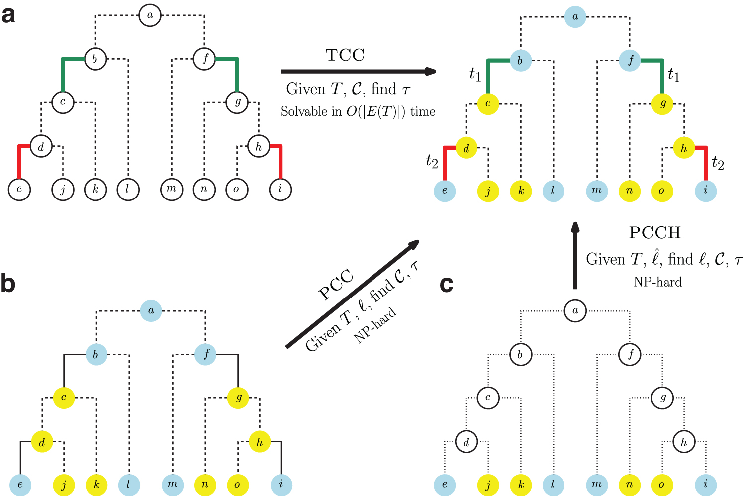
Outline of the three problems studied in this article. (a) Given a tree T and comigrations $C$ indicated by edge colors, the TCC problem seeks a timestamp labeling $τ$ that is temporally consistent with $C$ . Here, the timestamps $τ$ are represented by the edge labels, with $t_{1} = τ ((f, g)) = τ ((b, c)) < τ ((h, i)) = τ ((d, e)) = t_{2}$ ensuring temporal consistency. (b) Given a location labeling $ℓ$ (vertex colors) of a tree T, the PCC problem seeks a set $C$ of minimum-cardinality spatiotemporally consistent comigrations. Note that in both TCC and PCC, migrations (indicated by solid edges) and nonmigrations (indicated by dashed edges) are known and uniquely determined by $C$ and $ℓ$ , respectively. (c) Finally, given a tree T and a leaf labeling $\hat{ℓ}$ , the PCCH problem seeks a location labeling $ℓ$ that admits a minimum-cardinality set $| M (T, ℓ) |$ of migrations and subsequently induces the smallest, spatiotemporally consistent set $C$ of comigrations. PCC, parsimonious consistent comigrations; PCCH, parsimonious consistent comigration history; TCC, temporally consistent comigrations.

We formulate integer linear programs (ILPs) for exactly solving PCC and PCCH. We introduce a workflow for checking MACHINA migration histories for temporally consistency, and, if necessary, correcting them using the problems and algorithms introduced in this article. On simulated data, we find that MACHINA may fail to return temporally consistent solutions. On real data of metastatic cancers with relatively small phylogenetic trees, we find that MACHINA returned temporally consistent solutions. In summary, this work addresses a deficiency in a previous mathematical model of comigration, providing precise definitions and conditions for temporal consistency.

2. PROBLEM STATEMENT

We consider directed trees T rooted at a vertex $r (T)$ . We use the term edge to refer to a directed edge or arc, denoted as the pair $(u, v)$ where the vertex u is closest to the root $r (T)$ . Vertices of T are denoted by $V (T)$ , edges by $E (T)$ , and leaves by $L (T)$ . We use the term lineage to refer to root-to-leaf paths of T. To indicate that vertex u is an ancestor of vertex v, that is, there is a directed path from u to v, we write $u ≼_{T} v$ . We note that it holds that $v ≼_{T} v$ for all vertices v, that is, the relation $≼_{T}$ is reflexive. We denote the set of children of any vertex v by $δ (v)$ . To represent migration histories, we follow the work of Slatkin and Maddison (1989) and let $Σ$ be the set of all locations of origin and define a labeling $ℓ : V (T) \to Σ$ of the vertices of T by locations $Σ$ , called the location labeling, as follows.

Definition 1. A location labeling is a function $ℓ : V (T) \to Σ$ that labels the vertices of T with locations from $Σ$ .

Migrations are edges of T whose endpoints are assigned different locations by $ℓ$ .

Definition 2. A migration is an edge $(u, v) \in E (T)$ whose endpoints u and v have different locations, that is, $ℓ (u) \neq ℓ (v)$ . The set of all migrations of T induced by location labeling $ℓ$ is denoted by $M (T, ℓ)$ .

We say a location s is seeding a location t if there exists a migration $(u, v) \in M (T, ℓ)$ such that $ℓ (u) = s$ , $ℓ (v) = t$ , and $s \neq t$ . As mentioned previously, some evolutionary process allow for multiple migrations between the same pair of locations to occur in a single event. Thus, we wish to partition the set $M (T, ℓ)$ of migrations into set $C$ of comigrations rather than considering each migration in isolation.

Definition 3. A set $C$ of comigrations is a partition of a set $M \subseteq E (T)$ of migrations, that is, (i) each migration $(u, v) \in M$ occurs in exactly one part and (ii) the union of all parts $C \in C e q u a l s M$ .

For comigrations $C$ to be valid, all the migrations belonging to the same comigration needs to migrate between the same pair of locations at the same time. To that end, we define spatial and temporal consistency as follows.

Definition 4. A set $C$ of comigrations is spatially consistent with location labeling $ℓ$ if for all two migrations $(u, v), (u', v')$ in the same part $C \in C$ it holds that $ℓ (u) = ℓ (u')$ and $ℓ (v) = ℓ (v')$ .

To model temporal consistency, we first introduce a timestamp labeling that labels each migration by a timestamp defined as follows.

Definition 5. A timestamp labeling is a function $τ : M \to N$ that labels each migration of M with a timestamp.

We now define temporal consistency as follows.

Definition 6. A set $C$ of comigrations is temporally consistent with timestamp labeling $τ$ provided (i) all pairs $(u, v), (u', v')$ of migrations in the same part $C \in C$ have the same timestamp, that is, $τ ((u, v)) = τ ((u, v'))$ and (ii) $τ ((u, v)) < τ ((u', v'))$ for any two migrations $(u, v), (u', v')$ where $v ≼_{T} u'$ .

For the first problem, we focus on finding the chronological order of comigrations. That is, given a set $C$ of comigrations, we wish to identify a timestamp labeling $τ$ with which $C$ is temporally consistent.

Problem 1 (TCC). Given a rooted tree T and comigrations $C$ on migrations $M \subseteq E (T)$ , find a timestamp labeling $τ$ s.t. $C$ is temporally consistent with $τ$ .

We say that comigrations $C$ are temporally consistent if the corresponding TCC problem instance has a solution.

Next, we consider the problem where we are no longer given the set $C$ of comigrations but only the location labeling $ℓ$ and seek to identify temporally consistent comigrations $C$ . As there may be multiple possible scenarios, we seek the most parsimonious solution, that is, the solution with the fewest comigrations, leading to the following problem.

Problem 2 (PCC). Given a rooted tree T with location labeling $ℓ : V (T) \to Σ$ , find comigrations $C$ of migrations $M (T, ℓ)$ s.t. (i) $C$ is spatially consistent with $ℓ$ , (ii) $C$ is temporally consistent for some timestamp labeling $τ$ , and (iii) the number $| C |$ of comigrations is minimized.

We note that in practice, we are only given a leaf labeling $\hat{ℓ} : L (T) \to Σ$ as input, where each leaf $v \in L (T)$ is labeled with a location $\hat{ℓ} (v)$ from $Σ$ , rather than a location labeling that labels all vertices of T. In the third problem, we wish to infer the vertex labeling that corresponds to a most parsimonious solution for the given leaf labeling. Similarly to the problem solved by MACHINA (El-Kebir et al., 2018), we seek to find the solution that lexicographically minimizes the number of migrations and the number of comigrations. The key difference between the PCCH problem posed below and the previous problem solved by MACHINA is that here we explicitly enforce temporal consistency.

Problem 3 (PCCH). Given a rooted tree T with location leaf labeling $\hat{ℓ} : L (T) \to Σ$ , find location labeling $ℓ$ and comigrations $C$ of $M (T, ℓ)$ s.t. (i) $ℓ (v) = \hat{ℓ} (v)$ for all leaves $v \in L (T)$ , (ii) C is spatially consistent with $ℓ$ , (iii) there exist timestamps $τ$ temporally consistent with $C$ , and (iv) the number $| M (T, ℓ) |$ of migrations, and subsequently the number $| C |$ of comigrations is minimized.

To understand why we chose this particular ordering of the two objectives, note that there is a trade-off between the number of migrations and comigrations, where minimizing one objective comes at the expense of the other. Assuming that the location leaf labeling $\hat{ℓ}$ is injective, that is, for each location s in $Σ$ , there exists at least one leaf v such that $\hat{ℓ} (v) = s$ , it holds that the number $| C |$ of comigrations is at least $| Σ | - 1$ for any location labeling $ℓ$ and corresponding set $C$ of comigrations subject to conditions (i) and (ii) of the PCCH problem. To see why, observe that each location must be seeded or migrated into at least once except or the location at the root $r (T)$ . In other words, for each of the $s \in | Σ | ∖ {ℓ (r (T))}$ locations, there is at least one migration $(u, v) \in M (T, ℓ)$ such that $ℓ (u) \neq s$ and $ℓ (v) = s$ . There always exists a (temporally-consistent) location labeling with $| Σ | - 1$ comigrations, for example, labeling all the internal vertices with the same location.

Location labelings with $| Σ | - 1$ comigrations correspond to tree-like migration histories, with each location not equal to $ℓ (r (T))$ seeded by exactly one other location. To allow for more complex migration scenarios, we follow the problem statement introduced in El-Kebir et al. (2018) and minimize the number of migrations first and then comigrations. Note that the problem with the two objectives reversed, that is, minimizing comigrations first followed by migrations, was previously considered and shown to be NP-hard (El-Kebir, 2018).

3. COMBINATORIAL CHARACTERIZATION AND COMPLEXITY

This section includes the theoretical results on the combinatorial characteristics and complexity of the three discussed problems. The proofs have been moved to Appendix A (Supplementary Data) because of space constraints.

3.1. Combinatorial characterization of the TCC problem

To solve the TCC problem, we define the comigration graph $G_{T, C}$ , which is obtained from a tree T with comigrations $C$ as follows.

Definition 7. A comigration graph $G_{T, C}$ for a tree T with comigrations $C = {C_{1}, \dots, C_{| C |}}$ is a directed graph with vertices $V (G_{T, C}) = C$ and a directed edge $(C_{a}, C_{b}) \in E (G_{T, C})$ if there exist migrations $(u_{a}, v_{a}) \in C_{a}$ and $(u_{b}, v_{b}) \in C_{b}$ s.t. $v_{a} ≼_{T} u_{b}$ and $C$ does not contain any other migration on the path from v_a to u_b in T.

A comigration graph $G_{T, C}$ seeks to order comigrations $C$ by the placement of their corresponding migrations in T. More specifically, $G_{T, C}$ contains an edge $(C_{a}, C_{b})$ if and only if a migration from C_a immediately precedes a migration from C_b on the same root-to-leaf path in T. Note $G_{T, C}$ need not be connected (Fig. 2c). On the contrary, comigration graphs for migrations obtained by a location labeling do not contain self-loops.

FIG. 2.

Temporally inconsistent and consistent comigrations with comigration graphs. 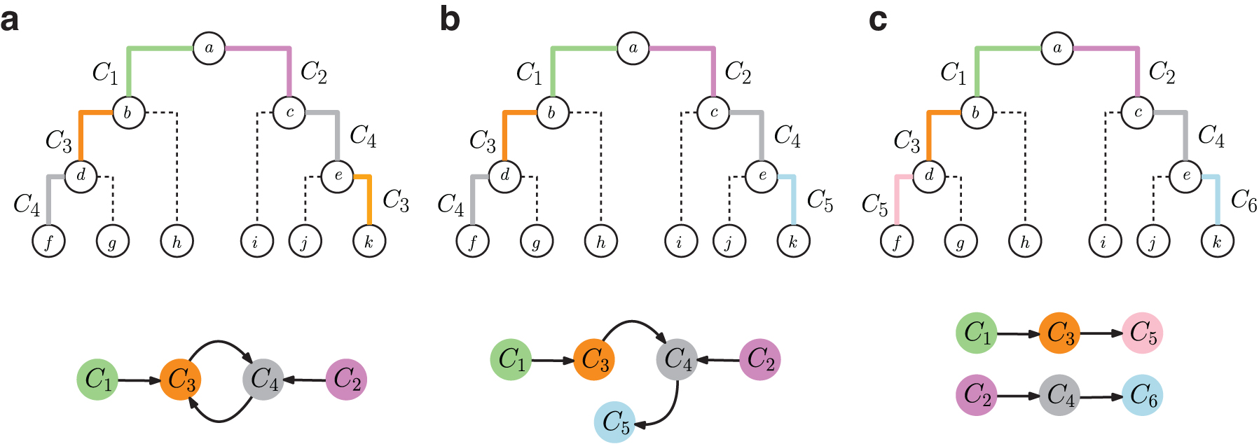(a–c) Three distinct sets of comigrations (edge colors) in the same tree with migrations (solid edges) and nonmigrations (dashed edges), resulting in different comigration graphs. (a) The comigration graph contains a directed cycle between C₃ and C₄, and therefore the corresponding set of comigrations is temporally inconsistent. (b, c) The comigration graphs are DAGs and, therefore, the corresponding sets of comigrations are temporally consistent. DAG, directed acyclic graph.

Lemma 1. There are no self-loops in the comigration graph $G_{T, C}$ of any set $C$ of comigrations for migrations $M (T, ℓ)$ induced by location labeling $ℓ$ of a tree T.

We have the following important theorem, stating that comigrations $C$ admit temporally consistent timestamps if and only if $G_{T, C}$ is a directed acyclic graph (DAG)—see Figure 2.

Theorem 1. There exists a timestamp labeling $τ$ that is temporally consistent with comigrations $C$ of a tree T if and only if the comigration graph $G_{T, C}$ is a DAG.

We show how to solve TCC in $O (| E (T) |)$ time in Section 4.1.

3.2. Relationship to MACHINA's comigrations

As we have mentioned earlier, MACHINA (El-Kebir et al., 2018) was the first method to incorporate comigrations in its problem formulation. Our notion of comigrations is similar to the one introduced in MACHINA (El-Kebir et al., 2018), but there are significant distinctions. MACHINA requires comigrations $C$ such that for each comigration $C \in C$ , all the migrations belonging to C migrate between the same pair of locations, and no two migrations from C are in the same root-to-leaf path. In other words, MACHINA considers comigrations $C$ to be valid if they maintain compatibility defined as follows.

Definition 8 (El-Kebir et al., 2018). Comigrations $C$ for migrations $M (T, ℓ)$ are compatible with location labeling $ℓ$ provided for any two migrations $(u, v), (u', v')$ in the same comigration $C \in C$ , it holds that (i) $ℓ (u) = ℓ (u')$ and $ℓ (v) = ℓ (v')$ , and (ii) neither $v ≼_{T} u'$ nor $v' ≼_{T} u$ .

The minimum number $γ (T, ℓ)$ of comigrations among all comigrations $C$ that are compatible with a fixed location labeling $ℓ$ can be computed as follows.

Lemma 2 (El-Kebir et al., 2018). The minimum number $γ (T, ℓ)$ of comigrations among all comigrations compatible with $ℓ$ equals

where $γ (T, ℓ, s, t)$ is the maximum number of migrations between locations $(s, t)$ on any root-to-leaf path of T.

While comigrations $C$ compatible with location labeling $ℓ$ are clearly spatially consistent, they may not be temporally consistent. We give one example in Figure 3 where the comigrations are compatible with the location labeling $ℓ$ but not temporally consistent. The following lemma relates our notions of spatial and temporal consistency (Definitions 4 and 6, respectively) with compatibility (Definition 8).

FIG. 3.

Comigrations inferred by MACHINA (El-Kebir et al., 2018) might not be temporally consistent. (a) Given the tree T and location labeling $ℓ$ with locations $Σ$ indicated by colors $Σ = {r e d, g r e e n, c y a n, o r a n g e}$ , comigrations ${C_{(r e d, g r e e n)}, C_{(c y a n, o r a n g e)}}$ indicated by gray boxes are compatible with $ℓ$ . However, assigning timestamps $τ$ such that $τ ((u'_{c y a n}, v'_{o r a n g e})) > τ ((u'_{r e d}, v'_{g r e e n}))$ violates temporal consistency as $(u'_{c y a n}, v'_{o r a n g e}) ≼_{T} (u'_{r e d}, v'_{g r e e n})$ . A similar violation happens if the timestamp of $C_{(c y a n, o r a n g e)}$ precedes that of $C_{(r e d, g r e e n)}$ instead. To get comigrations that are temporally consistent, we must break up either (b) $C_{(r e d, g r e e n)}$ or (c) $C_{(c y a n, o r a n g e)}$ , leading to an additional comigration in either case.

Lemma 3. Comigrations $C$ for migrations $M (T, ℓ)$ that are spatially and temporally consistent with location labeling $ℓ$ of a tree T are also compatible with $ℓ$ .

The following corollary directly follows from Lemma 2 and Lemma 3.

Corollary 1. Comigrations $C$ that are spatially and temporally consistent with location labeling $ℓ$ of a tree T consist of at least $| C | \geq γ (T, ℓ)$ parts.

Note that MACHINA only computes the number $γ (T, ℓ)$ of comigrations and does not explicitly infer the corresponding comigrations $C^{*}$ s.t. $| C^{*} | = γ (T, ℓ)$ . We present a simple greedy algorithm, denoted as Greedy-Comigrations $(T, ℓ)$ , to infer $C^{*}$ . In brief, the algorithm starts with $C^{*} = {C_{1}, \dots, C_{| M (T, ℓ) |}}$ , where each comigration $C \in C^{*}$ contains exactly one unique migration from $M (T, ℓ)$ . Then in each iteration, two distinct parts C and $C'$ are merged in $C^{*}$ if all the migrations from C and $C'$ are between the same pair of locations and exist in distinct root-to-leaf paths in T. The algorithm continues until no more comigration pairs can be merged. We refer to Algorithm 2 in Appendix B.1 for pseudocode more formally describing this algorithm. Note that the algorithm maintains compatibility as a loop invariant, which ensures correctness.

Lemma 4. For any rooted tree T and location labeling $ℓ$ , Greedy-Comigrations $(T, ℓ)$ infers comigrations $C^{*}$ for $M (T, ℓ)$ s.t. (i) $C^{*}$ is compatible with $ℓ$ and (ii) $| C^{*} | = γ (T, ℓ)$ .

Note that the greedy approach is not guaranteed to output comigrations that are both compatible with location labeling $ℓ$ and temporally consistent, even if there exist compatible comigrations $C$ for a given tree T and location labeling $ℓ$ such that $| C | = γ (T, ℓ)$ . One such example is discussed in Appendix B.1 and Supplementary Figure S1.

Finally, we explore a sufficient condition under which compatible comigrations $C$ exhibit temporal consistency. We say a location labeling $ℓ$ results in reseeding if there exists k distinct migrations $(u_{1}, v_{1}), \dots, (u_{k}, v_{k})$ such that $ℓ (v_{i}) = ℓ (u_{i + 1})$ for any $1 \leq i \leq k$ and $ℓ (u_{1}) = ℓ (v_{k})$ . In other words, the directed multigraph formed by vertices $Σ$ and containing a directed edge $[ℓ (u), ℓ (v)]$ for each migration $(u, v) \in M (T, ℓ)$ —called migration graph in El-Kebir et al. (2018)—is acyclic. We show that comigrations $C$ compatible with a location labeling $ℓ$ that does not result in reseeding are temporally consistent in the following proposition.

Proposition 1. If a location labeling $ℓ$ of a tree T does not result in reseeding then any set $C$ of comigrations on $M (T, ℓ)$ that is compatible with $ℓ$ is also temporally consistent.

This means that versions of MACHINA that restrict location labeling $ℓ$ to not have reseeding, including versions that only support tree-like migration patterns with $| Σ | - 1$ comigrations (El-Kebir, 2018), return temporally consistent solutions, although the solution may be suboptimal for the original unrestricted problem. Similarly, TiTUS (Sashittal and El-Kebir, 2020), which considers timed phylogenetic trees and imposes tree-like migration constraints (i.e., each location is seeded by at most one other location), will result in temporally consistent solutions.

In conclusion, MACHINA does not guarantee temporal consistency unless the inferred location labeling is reseeding-free. We will make use of this when developing a workflow for solving the PCCH problem in Section 4.4.

3.3. NP-hardness of the PCC problem

The example in Figure 3 and Lemma 1 demonstrates that the smallest set $C$ of TCC can have more comigrations than the polynomial-time computable lower bound $γ (T, ℓ)$ . In this section, we explore the complexity of PCC, which seeks the smallest set $C$ of temporally consistent comigrations for migrations $M (T, ℓ)$ induced by a location labeling $ℓ$ of a tree T. We have the following hardness result.

Theorem 2. PCC is NP-hard when $| Σ | \geq 3$ .

We prove this by a reduction from shortest common supersequence (SCS) in polynomial time. The SCS problem takes as input a set ${S_{1}, \dots, S_{n}}$ of n sequences, where each sequence S_i is an ordered list $s_{i, 1} s_{i, 2} \dots s_{i, | S_{i} |}$ of symbols from a finite set $S$ . We say sequence Y is a supersequence of sequence X if there exists a function $F_{X, Y} : {1, \dots, | X |} \to {1, \dots, | Y |}$ such that $F_{X, Y} (i) = j$ if $X_{i} = Y_{j}$ and F is a strictly increasing monotone function. The goal of the SCS problem is to find the shortest sequence $S^{*}$ such that $S^{*}$ is a supersequence of all input sequences $S_{1}, \dots, S_{n}$ . The SCS problem is NP-hard when $| S | \geq 2$ (Räihä and Ukkonen, 1981). We describe a polynomial time reduction from SCS to PCC. To that end, we build a tree T with location set $Σ = S \cup {⊥}$ and location labeling $ℓ : V (T) \to [S \cup {⊥}]$ given the input sequences $S_{1}, \dots, S_{n}$ in polynomial time. The construction is described below.

1.
Add the root o to the empty tree T and set the label of root o to be $ℓ (o) = ⊥$ . For convenience, The root o may also be represented as $o_{i, 0}$ for any $1 \leq i \leq n$ .
2.
For each input sequence S_i, attach the path $a_{i, 1}, o_{i, 1}, \dots, a_{i, | S_{i} |}, o_{i, | S_{i} |}$ of length $2 | S_{i} |$ to the root o. Vertices $a_{i, j}$ are referred to as a-vertices, while vertices $o_{i, j}$ are referred to as o-vertices. By construction, the edges in the tree T are either from an o-vertex to an a-vertex or from an a-vertex to an o-vertex. These are, respectively, called o-a edges and a-o edges.
3.
Label each a-vertex $a_{i, j}$ with $ℓ (a_{i, j}) = s_{i, j}$ and each o-vertex $o_{i, j}$ with $ℓ (o_{i, j}) = ⊥$ . Since $s_{i, j} \neq ⊥$ for all $i \in [n]$ and $j \in {1, \dots, | S_{i} |}$ , each edge of the tree T is a migration.

The lower bound of $| Σ | \geq 3$ in Theorem 2 is established by combining the facts that $Σ = S \cup {⊥}$ in the PCC instance corresponding to an SCS instance with set $S$ of symbols, and SCS is NP-hard when $| S | \geq 2$ . Figure 4 shows an example reduction.

FIG. 4.
Reduction from SCS to PCC. (a) Given an SCS problem instance with $n = 4$ sequences $S_{1}, S_{2}, S_{3}, S_{4}$ , we have the SCS $S^{} = s_{1}^{} \dots s_{m^{}}^{}$ of length $m^{} = | S^{} | = 5$ . The solution is illustrated as an alignment such that $s_{i, j}$ , the jth character of sequence i, is in column p if $s_{i, j}$ matches with the p-th character $s_{p}^{}$ of $S^{}$ . (b) The corresponding tree T with location labeling $ℓ$ on $Σ = {⊥, C, A, R, T}$ is shown. Each a-vertex $a_{i, j}$ is labeled by location $ℓ (a_{i, j}) = s_{i, j}$ , with the color matching (a), and each o-vertices $o_{i, j}$ is labeled by locations $ℓ (o_{i, j}) = ⊥$ and are colored white. The corresponding set $C$ of $2 m^{} = 2 \cdot 5 = 10$ comigrations is indicated by gray boxes, with migrations/edges overlapping a gray box belonging to the same part of $C$ . SCS, shortest common supersequence.

In the following, let $(T, ℓ)$ be the PCC instance obtained from SCS instance ${S_{1}, \dots, S_{n}}$ . Moreover, we denote with $C^{}$ any optimal solution of the PCC instance, that is, $C^{}$ is a set of comigrations that is spatially consistent with $ℓ$ , temporally consistent, and minimizes the number $| C^{} |$ of comigrations. We have the following definition.

Definition 9. A set $C$ of comigrations for migrations $M (T, ℓ) = E (T)$ is balanced if $C$ consists of an even number of parts, half of which comprised only o-a edges and the other half comprised only a-o edges.

Lemma 5. Any optimal set $C^{}$ of comigrations that is spatially and temporally consistent with location labeling* $ℓ$ of T is balanced.

Next, we show that there exists a mapping between supersequences S of length m and balanced sets $C$ of $2 m$ spatiotemporally consistent comigrations.

Lemma 6. There exists a common supersequence $S = s_{1} \dots s_{m}$ of ${S_{1}, \dots, S_{n}}$ if and only if there exists a balanced set $C$ of comigrations with $| C | = 2 m$ parts that is spatially and temporally consistent with location labeling $ℓ$ of T.

Finally, we prove the following lemma from which Theorem 2 follows.

Lemma 7. There exists a SCS $S^{} = s_{1}^{} \dots s_{m^{}}^{}$ of ${S_{1}, \dots, S_{n}}$ if and only if there exists a minimum-cardinality set $C^{}$ of comigrations for migrations* $M (T, ℓ) = E (T)$ that is spatially and temporally consistent with $ℓ$ and has $| C^{} | = 2 m^{}$ parts.
3.4. NP-hardness of the PCCH problem

In this subsection, we prove PCCH to be NP-hard.

Theorem 3. PCCH is NP-hard when $| Σ | \geq 3$ .

We show that PCCH is NP-hard by reduction from PCC. To that end, given a tree T with location labeling $ℓ$ , we construct another tree $T'$ with leaf labeling $\hat{ℓ}'$ . The steps are as follows.

1.
For every vertex $v \in V (T)$ , add a vertex $v'$ to $V (T')$ .
2.
For every edge $(u, v) \in E (T)$ , add an edge $(u', v')$ to $E (T')$ .
3.
For every leaf $v \in L (T)$ , keep its label $ℓ (v)$ for the corresponding vertex $v'$ in $T'$ , that is, $\hat{ℓ}' (v') = ℓ (v)$ .
4.
For each internal vertex $v \in V (T) ∖ L (T)$ with degree $d e g (v)$ , attach $d e g (v) + 1$ leaves ${v'_{1}, \dots, v'_{d e g (v) + 1}}$ to vertex $v'$ of $T'$ , labeling each of these leaves with $ℓ (v)$ , that is, $\hat{ℓ}' (v'_{i}) = ℓ (v)$ for $i \in {1, \dots, d e g (v) + 1}$ .

Clearly, the reduction described above takes polynomial time. Note that the set $Σ$ of locations is the same for both the PCC instance and the corresponding PCCH instance. Therefore, our hardness result for PCCH has the same bound $| Σ | \geq 3$ as in Theorem 2 establishing hardness for PCC. We give an example construction in Supplementary Figure S2.

Given the constructed tree $T'$ with leaf labeling $\hat{ℓ}'$ from PCC instance $(T, ℓ)$ , PCCH aims to find the location labeling $ℓ'$ as well as spatially and TCC $C'$ that result in the minimum number $| M (T', ℓ') |$ of migrations and subsequently the minimum number $| C' |$ of comigrations. The reduction ensures that an optimal location labeling $ℓ'$ assigns the same locations to internal vertices of $T'$ as location labeling $ℓ$ does to the corresponding internal vertices v of T, as we show in the following lemma.

Lemma 8. For each vertex $v \in V (T)$ , an optimal location labeling $ℓ'$ of $T'$ labels the corresponding vertex $v'$ as $ℓ' (v') = ℓ (v)$ .

The previous lemma means that the number $| M (T', ℓ') |$ of migrations is fixed for optimal location labelings $ℓ'$ .

Corollary 2. The number $| M (T', ℓ') |$ of migrations for an optimal location labeling $ℓ'$ of $T'$ equals the number $| M (T, ℓ) |$ of migrations in T with location labeling $ℓ$ .

Finally, we prove the main lemma from which hardness follows.

Lemma 9. Let $(T, ℓ)$ be a PCC instance with $| M (T, ℓ) | = μ$ and $(T', \hat{ℓ}')$ be the corresponding PCCH instance. There exists an optimal solution $C$ for $(T, ℓ)$ s.t. $| C | = γ$ if and only if there exists an optimal solution $(ℓ', C')$ for $(T', \hat{ℓ}')$ s.t. $| M (T', ℓ') | = μ$ and $| C' | = γ$ .
4. METHODS

In this section, we introduce algorithms to solve the three problems we discussed, and also introduce a workflow for inferring a temporally consistent migration history from input trees with leaf labeling.

4.1. Linear time algorithm for the TCC problem

The proof of Theorem 1 describes a way of solving TCC by computing a topological ordering of the vertices of the given comigration graph $G_{T, C}$ . A topological ordering is a linear ordering of the comigration graph's vertices such that for every edge $(u, v)$ vertex u comes before v in the ordering; such an ordering exists if and only if $G_{T, C}$ is a DAG. Given a topological ordering $t : C \to {1, \dots, | C |}$ of the vertices $V (G_{T, C}) = C$ , we can obtain timestamps $τ : M \to N$ by setting $τ ((u, v)) = t (C)$ if the migration $(u, v) \in C$ where C is a comigration in the set $C$ of comigrations. Using Kahn's algorithm (Kahn, 1962), we can obtain the topological ordering in time $O (| V (G_{T, C}) | + | E (G_{T, C}) |)$ . Since the number $| C |$ of comigrations can be at most the number $| M |$ of migrations, which in turn can be at most the number $| E (T) |$ of edges in tree T, we have $| V (G_{T, C}) | = | C | = O (| E (T) |)$ . The following lemma provides a bound for $| E (G_{T, C}) |$ .

Lemma 10. The number of edges in comigration graph $G_{T, C}$ is at most the number of edges in T, that is, $| E (G_{T, C}) | = O (| E (T) |)$ .

Thus, by Lemma 10, TCC can be solved in $O (| V (G_{T, C}) | + | E (G_{T, C}) |) = O (| E (T) |)$ time if $G_{T, C}$ is given. We still need to show how to construct the comigration graph $G_{T, C}$ itself. One naive way to construct $G_{T, C}$ is by checking each pair $(u, v), (u', v') \in M$ of migrations, and adding edge $(C_{s}, C_{t})$ to $G_{T, C}$ if $(u, v) \in C_{s}$ , $(u', v') \in C_{t}$ , $v ≼_{T} u'$ , and there is no migration on the path from v to $u'$ . But this approach requires quadratic time, so we propose a new linear-time algorithm. The recursive algorithm BuildComigrationGraph $(T, M, C, v)$ takes as input a tree T, set M of migrations, set $C$ of comigrations, and a vertex $v \in V (T)$ . It returns two outputs: (i) a comigration graph denoted as $G_{T_{v}, C}$ such that an edge $(C_{s}, C_{t})$ exists if there are two migrations $(u, v) \in C_{s}$ and $(u', v') \in C_{t}$ in the subtree T_v rooted at v, and (ii) a subset $X_{v} \subseteq C$ of comigrations such that $C \in X_{s}$ if C includes a migration $(u', v')$ that is the first migration encountered on a directed path from v to any leaf. Since $T_{r (T)} = T$ , BuildComigrationGraph $(T, M, C, r (T))$ infers the comigration graph $G_{T, C}$ . The pseudocode is given in Algorithm 1 in Appendix A.1.

Theorem 4. BuildComigrationGraph $(T, M, C, r (T))$ returns comigration graph $G_{T, C}$ in $O (| E (T) |)$ time.

4.2. ILP for the PCC problem

In the previous section, we have shown that PCC is NP-hard. We solve the problem to optimality using an ILP. To solve the problem to optimality, we formulate an ILP, modeling comigrations $C$ and timestamp labeling $τ$ for the given set $M (T, ℓ)$ of migrations induced by a given location labeling $ℓ$ of a given tree T. The objective is to minimize the number $| C |$ of comigrations while ensuring that $C$ is spatiotemporally consistent.

4.2.1. Timestamp labeling

First, we begin by noting that the number of unique timestamps is at most the number $| M (T, ℓ) |$ of migrations. Thus, we enumerate all possible timestamps as ${1, \dots, | M (T, ℓ) |}$ . To model the assignment of timestamps $τ ((u, v))$ to migration edges $(u, v) \in M (T, ℓ)$ , we introduce binary variables $x \in {0, 1}^{M (T, ℓ) \times | M (T, ℓ) |}$ such that $x_{(u, v), e}$ is 1 if $τ ((u, v)) = e$ and 0 otherwise. We have the following corresponding constraints, ensuring each migration edge is assigned one timestamp.

For any two migrations $(u, v), (u', v') \in M (T, ℓ)$ where $v ≼_{T} u'$ , we require $τ ((u, v)) < τ ((u', v'))$ by the definition of temporal consistency (Definition 6). Now if $τ ((u, v)) < τ ((u', v'))$ then for any $τ ((u, v)) \leq E < τ ((u', v'))$ we have $\sum_{e = 1}^{E} x_{(u, v), e} > \sum_{e = 1}^{E} x_{(u', v'), e}$ . Conversely, if $E < τ ((u, v))$ or $E \geq τ ((u', v'))$ then $\sum_{e = 1}^{E} x_{(u, v), e} = \sum_{e = 1}^{E} x_{(u', v'), e}$ . We combine these two conditions to form the following constraints.

where $π (T, ℓ)$ consists of all ordered pairs $((u, v), (u', v'))$ of migrations s.t. (i) $(u, v), (u', v') \in M (T, ℓ)$ , (ii) $v ≼_{T} u'$ , and (iii) there is no migration in the path from v to $u'$ . Note that the third condition is not necessary but results in fewer constraints, potentially speeding up the ILP.

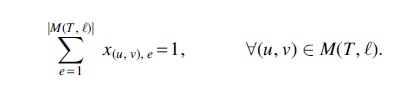
4.2.2. Comigrations

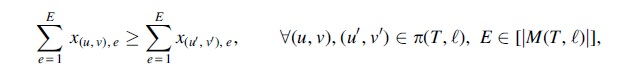
For spatiotemporally consistent comigrations $C$ , each part $C \in C$ consists of migrations between the same pair of locations indicated by $ℓ$ that have the same timestamp given by a timestamp labeling $τ$ . In general, one may use the same timestamp for two comigrations occurring between distinct pairs of locations. However, in this formulation, we will require each comigration to have a unique timestamp, which we use to identify the comigration. This is without loss of generality because one can relabel any temporally consistent $τ$ to use unique timestamps maintaining temporal consistency. Thus, to model comigrations, we introduce binary variables $x \in {0, 1}^{| M (T, ℓ) | \times Σ \times Σ}$ , where $y_{e, s, t} = 1$ if there exists at least one migration $(u, v)$ such that $ℓ (u) = s, ℓ (v) = t$ , and $τ ((u, v)) = e$ , and $y_{e, s, t} = 0$ otherwise. We have the following constraints ensuring that each timestamp corresponds to at most one comigration.

For each migration $(u, v)$ with timestamp $τ ((u, v)) = e$ , we force $y_{e, ℓ (u), ℓ (v)}$ to be 1 as follows. $y_{e, ℓ (u), ℓ (v)} \geq x_{(u, v), e}, \forall (u, v) \in M (T, ℓ), \forall e \in [| M (T, ℓ) |] .$

4.2.3. Symmetry-breaking constraints

To increase performance, we use symmetry breaking constraints enforcing smaller timestamps to be used first.

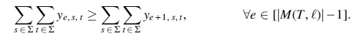
4.2.4. Optimization function

Since we require each comigration to have a unique timestamp, the total number of comigrations equals the number of nonzero entries in y.

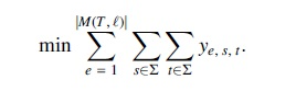
Note that the objective function will ensure that $y_{e, s, s} = 0$ for all timestamps $e \in [| M (T, ℓ) |]$ and $s \in Σ$ .

4.2.5. Model size

PCC's ILP consists of variables and $O (| M (T, ℓ) |^{2}) = O (| E (T) |^{2})$ constraints.

4.3. ILP for the PCCH problem

In the previous section, we showed PCCH to be NP-hard. We solve the problem to optimality using an ILP. To do so, we must model (i) a location labeling $ℓ$ , (ii) comigrations $C$ identified by the labels of endpoints and timestamps of the member edges, (iii) an assignment of edges to parts, and (iv) symmetry-breaking constraints. The details of each step are discussed as follows.

4.3.1. Location labeling

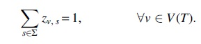
To model location labeling $ℓ$ , we introduce binary variables $z \in {0, 1}^{V (T) \times Σ}$ such that $z_{v, s} = 1$ if $ℓ (v) = s$ , and $z_{v, s} = 0$ otherwise. As each vertex must be labeled by a location, we have

In addition, for the leaves of T, we force location labeling $ℓ$ to match with input leaf labeling $\hat{ℓ}$ . $z_{v, \hat{ℓ} (v)} = 1, \forall v \in L (T) .$

4.3.2. Timestamp labeling

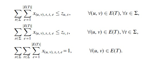
For efficient ILP formulation, we assign timestamps on nonmigrations and include them in comigrations. This modification does not change the original PCCH algorithm, as the timestamps on nonmigrations can be ignored while still ensuring temporal consistency. Again the number of distinct comigrations and thus timestamps is at most the number $| E (T) |$ of edges, allowing us to enumerate our timestamps as ${1, \dots, | E (T) |}$ . Like our ILP for PCC, we introduce binary variables $x \in {0, 1}^{E (T) \times Σ \times Σ \times | E (T) |}$ s.t. $x_{(u, v), s, t, e}$ is 1 if $ℓ (u) = s$ , $ℓ (v) = t$ , and $τ ((u, v)) = e$ , and $x_{(u, v), s, t, e} = 0$ otherwise. These described conditions are enforced by the following three conditions.

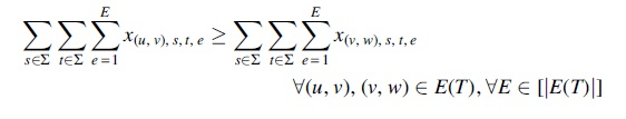
To ensure temporal consistency, for any two consecutive edges $(u, v), (v, w) \in E (T)$ , we require the timestamp of $(u, v)$ to be smaller than the timestamp of $(v, w)$ .

4.3.3. Comigrations

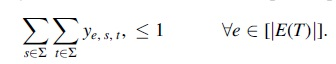
Similar to our ILP for PCC, we again require each comigration to have a unique timestamp and use the timestamps to identify individual comigrations in this ILP. To that end, we introduce binary variables $y \in {0, 1}^{| E (T) | \times Σ \times Σ}$ where $y_{e, s, t} = 1$ if there exists a migration $(u, v)$ such that $ℓ (u) = s$ , $ℓ (v) = t$ , and $τ ((u, v)) = e$ , and $y_{e, s, t} = 0$ otherwise. The following constraint ensures spatial consistency by enforcing each comigration to be associated with a specific pair of locations.

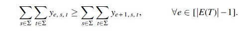
For each edge $(u, v)$ with $ℓ (u) = s$ , $ℓ (v) = t$ , and $τ ((u, v)) = e$ , we force $y_{e, s, t}$ to be 1. $x_{(u, v), s, t, e} \leq y_{e, s, t}, \forall (u, v) \in E (T), \forall s, t \in Σ, \forall e \in [| E (T) |] .$

4.3.4. Symmetry-breaking constraints

Like the ILP model for PCC, we eliminate some symmetrical solutions by forcing smaller partition numbers to be used first.

4.3.5. Optimization function

We compute the number of migrations from variables x by counting the number of migrations. Since we ignore the comigrations with nonmigrations, we only count the number of comigrations that contain migrations from variables y. Thus, we define the objective function as

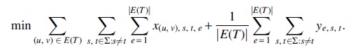
In the optimization function, the factor $\frac{1}{| E (T) |}$ ensures that the ILP first minimizes the number of migrations and then the number of comigrations.

4.3.6. Model size

PCCH's ILP consists of $O (| E (T) |^{2} | Σ |^{2})$ variables and $O (| E (T) |^{2} (| E (T) |^{2} | + | Σ |^{2})) = O (| E (T) |^{4})$ constraints.

4.4. Workflow for inferring temporally consistent migration histories

MACHINA, like PCCH, employs an ILP for migration history inference. While both methods minimize migrations and comigrations lexicographically, MACHINA does not enforce temporal consistency like PCCH, resulting in a simpler ILP with 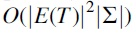$O (| E (T) |^{2} | Σ |)$ variables and $O (| E (T) |^{2} | Σ |)$ constraints, considerably fewer than PCCHs ILP with variables and $O (| E (T) |^{4})$ constraints. Due to the increased size of PCCHs ILP, we expect it to be slower compared to MACHINA. Furthermore, as per Proposition 1, MACHINA is guaranteed to infer optimal TCC when there is no reseeding. Therefore, we propose a workflow for migration history inference that leverages MACHINA's speed whenever feasible and ensures temporal consistency in the solutions by falling back to PCC and PCCH when necessary.

The workflow has five steps in total (Fig. 5). In step I, given an input tree T and leaf labeling $\hat{ℓ}$ , we run MACHINA to obtain a location labeling $ℓ_{M A C H I N A}$ with the minimum number $γ (T, ℓ_{M A C H I N A})$ of compatible comigrations. For step II, we note that MACHINA does not explicitly output the comigrations. If one is not interested in this set of comigrations but only the number of comigrations, we can use Proposition 1 and check whether $ℓ_{M A C H I N A}$ is reseeding-free, and if so, only report the number $γ (T, ℓ_{M A C H I N A})$ of comigrations. Therefore, we run Greedy-Comigrations to get the set of compatible comigrations $C_{M A C H I N A}$ such that $| C_{M A C H I N A} | = γ (T, ℓ_{M A C H I N A})$ . In step III, we run the TCC algorithm to check whether $C_{M A C H I N A}$ is temporally consistent. If $C_{M A C H I N A}$ is temporally consistent then, by Corollary 1, $C_{M A C H I N A}$ is optimal and we terminate.

FIG. 5.

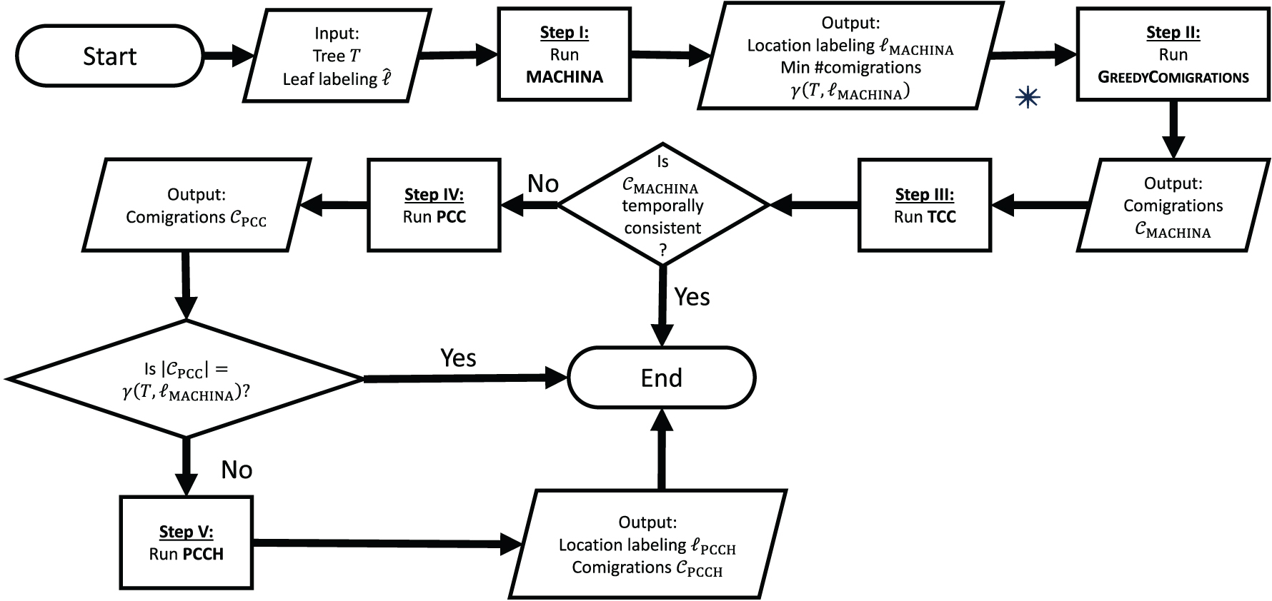
Workflow for inferring temporally consistent migration histories. The workflow consists of sequentially running MACHINA and the algorithms discussed in this article, falling back on more complex algorithms whenever necessary. *In case the user is not interested in the specific set $C_{M A C H I N A}$ of comigrations but only the number of comigrations, one can utilize Proposition 1 and check whether $ℓ_{M A C H I N A}$ is reseeding-free, and if so, report the number $γ (T, ℓ_{M A C H I N A})$ of comigrations.

Otherwise if $C_{M A C H I N A}$ is temporally inconsistent, we proceed to step IV. In this step, we run the PCC ILP on input tree T and MACHINA location labeling $ℓ_{M A C H I N A}$ to obtain the minimum set $C_{P C C}$ of TCC. Since Greedy-Comigrations does not guarantee $C_{M A C H I N A}$ to be temporally consistent, PCC helps checking whether there exists a temporally consistent set $C_{P C C}$ of comigrations such that $| C_{P C C} | = γ (T, ℓ_{M A C H I N A})$ . If $| C_{P C C} | = γ (T, ℓ_{M A C H I N A})$ then the location labeling $ℓ_{M A C H I N A}$ combined with the spatially consistent comigrations $C_{P C C}$ form an optimal solution to the PCCH (Corollary 1), thus allowing us to terminate the workflow. Otherwise, if $| C_{P C C} | > γ (T, ℓ_{M A C H I N A})$ , we proceed with step V. In this final step, we run the PCCH ILP to compute the optimal location labeling $ℓ_{P C C H}$ along with the minimum temporally consistent set $C_{P C C H}$ of comigrations.

5. RESULTS

In this section, we compare the performance of MACHINA with our methods on simulated (Section 5.1) and real data (Section 5.2). All experiments were run on a server with Intel Xeon Gold 5120 dual CPUs with 14 cores each at 2.20 GHz and 512 GB RAM. The code, which uses Gurobi to solve the ILPs, as well as simulation and real data instances are available at https://github.com/elkebir-group/PCCH.

5.1. Simulated data

This section aims to evaluate the performance of our algorithms relative to MACHINA. To that end, we generated simulation instances following a three-step process. First, we sampled a comigration graph G resulting in a set $V (G) = C$ of comigrations. Second, we sampled a tree $T'$ with location labeling $ℓ$ and assigned migrations $M (T', ℓ)$ to the comigrations $C$ such that $T'$ and $C$ induced the edges of the sampled comigration graph, that is, G is a subgraph of $G_{T, C}$ . We imposed an additional condition ensuring that each part of $C$ consists of migrations that occur on distinct lineages. Third, we obtained the final tree T with leaf labeling $\hat{ℓ}$ by adding edges to $T'$ in a manner that minimizing the number of migrations and subsequently the number of compatible comigrations would yield the simulated comigrations $C$ .

We generated three classes of simulation instances, with increasing complexity in the initially sampled comigration graphs in the form of cycles. The details are provided in Supplementary Section D.1 and Supplementary Figure S3. We ran all five steps of the workflow for each instance without terminating prematurely. Thus, we ran MACHINA on each simulation instance $(T, \hat{ℓ})$ resulting in a location labeling $ℓ_{M A C H I N A}$ . We then used Greedy-Comigrations to extract the set $C_{M A C H I N A}$ of comigrations from $(T, ℓ_{M A C H I N A})$ . Next, we checked whether $C_{M A C H I N A}$ was temporally consistent using the TCC algorithm. In addition, we ran the PCC algorithm on the output $(T, ℓ_{M A C H I N A})$ produced by MACHINA, yielding a parsimonious set $C_{P C C}$ of TCC. Finally, we ran the PCCH algorithm on the original simulation instance $(T, \hat{ℓ})$ resulting in a location labeling $ℓ_{P C C H}$ and set $C_{P C C H}$ of comigrations. To assess the performance, we compared the outputs of each method, and also running times.

For our first set of simulations, we sampled five comigration graphs without any cycles, obtaining a total of five instances $(T, \hat{ℓ})$ , one for each sampled comigration graph. These instances had 26 to 74 vertices and included 3 to 7 locations. We expect all methods to yield temporally consistent solutions with identical numbers of migration and comigrations for these instances. Indeed, for each instance, we observed that $| M (T, ℓ_{M A C H I N A}) | = | M (T, ℓ_{P C C H}) |$ , $| C_{M A C H I N A} | = | C_{P C C} | = | C_{P C C H} |$ , and that MACHINA's solution was temporally consistent (Fig. 6a). Note that the $C_{P C C}$ and $C_{P C C H}$ are by definition temporally consistent. In terms of running time, MACHINA outperformed PCCH slightly, with median running times of 12.029 seconds for MACHINA and 18.806 seconds for PCCH (Fig. 6b). Despite PCCs NP-hardness, the corresponding ILP executed much faster than MACHINA and PCCH due to fewer constraints and variables in the ILP model, with a median running time of 0.043 seconds (Fig. 6b and Supplementary Table S4).

FIG. 6.

Simulation results. (a) The inferred numbers of comigrations (y-axis) for each method (color) across simulation instances (x-axis), additionally indicating temporal consistency (shape). (b) The running time (y-axis) for each method (color) across simulation instances (x-axis). (c–f) One simulation instance $(T, \hat{ℓ})$ where MACHINA fails to return a temporally consistent solution is included here, with (c) showing the MACHINA location labeling $ℓ_{M A C H I N A}$ and (d) the corresponding comigration graph $G_{T, C_{M A C H I N A}}$ containing several cycles (dashed). (e) By contrast, PCCH infers a location labeling $ℓ_{P C C H}$ that differs at the indicated vertex (“*”) and TCC $C_{P C C H}$ , (f) not containing any cycles in the induced comigration graph $G_{T, C_{P C C H}}$ . Note that while for both solutions, we have $| C_{M A C H I N A} | = 9 < 10 = | C_{P C C H} |$ .

We also executed our workflow on all five instances, which terminated at step III because of $C_{M A C H I N A}$ being temporally consistent (Supplementary Table S4). As the workflow skipped steps IV and V (PCC and PCCH), and the combined running time for steps II and III (Greedy-Comigrations and TCC) was significantly shorter, with a median of 0.002 seconds, the workflow's running time closely matched that of MACHINA (Fig. 6b and Supplementary Table S4).

To generate the second set of simulation instances, we picked comigration graphs with $k \in {1, 2, 3, 4}$ disjoint cycles. For each value of k, we generated five comigration graphs with k cycles and simulated five instances $(T, \hat{ℓ})$ , totaling 20 instances. The simulated trees had 26 to 88 vertices and 3 to 11 locations. Because of the presence of cycles in the initially sampled comigration graphs, MACHINA failed to return a temporally consistent set $C_{M A C H I N A}$ of comigrations for all the instances (Fig. 6a and Supplementary Table S4). As such, the number of comigrations inferred by MACHINA, PCC, and PCCH differed, although the number of migrations inferred by MACHINA matched that of PCCH. To be more specific, for the instances generated from initially sampled comigration graphs with $k \in {1, 2, 3, 4}$ cycles, MACHINA underestimated the minimum number of comigrations by k, that is, $| C_{M A C H I N A} | = | C_{P C C} | - k$ (Supplementary Table S4).

Note that MACHINA's inability to accurately determine the number of comigrations for a specific instance does not necessarily imply that the associated location labeling is incorrect. For example, in 9 out of 20 cases, $ℓ_{M A C H I N A}$ matched $ℓ_{P C C H}$ , and $C_{P C C}$ computed from $ℓ_{M A C H I N A}$ inferred by PCC matched $C_{P C C H}$ computed by PCCH. But in the other 11 cases, $| C_{P C C} |$ was greater than $| C_{P C C H} |$ , indicating that achieving the minimum comigration count with $ℓ_{M A C H I N A}$ was not possible, rendering $ℓ_{M A C H I N A}$ suboptimal (Fig. 6a and Supplementary Table S4). In these cases, we observed 1 to 3 vertices to be labeled differently between $ℓ_{M A C H I N A}$ and $ℓ_{P C C H}$ .

In Figure 6, we present a simulation instance with $k = 2$ cycles where MACHINA and PCCH produced different results. This instance corresponds to a tree T with 36 vertices and 5 locations. MACHINA provided the location labeling $ℓ_{M A C H I N A}$ shown in Figure 6c, reporting 15 migrations and 9 comigrations. However, the corresponding comigration graph $G_{T, C_{M A C H I N A}}$ in Figure 6d revealed two disjoint cycles, indicating temporal inconsistency in MACHINA's comigrations (Theorem 1). Running PCC on the location labeling $ℓ_{M A C H I N A}$ inferred by MACHINA deduced the minimum set $C_{P C C}$ of TCC to be of size 11. Conversely, PCCHs location labeling $ℓ_{P C C H}$ , depicted in Figure 6e, accounted for 15 migrations and 10 comigrations, with the corresponding comigration graph $G_{T, C_{P C C H}}$ in Figure 6f being a DAG. So the location labeling $ℓ_{P C C H}$ minimizes the number of TCC, and the solution returned by MACHINA is temporally inconsistent and suboptimal.

Although MACHINA was faster in $k = 1$ cases (median: 16.56 seconds for MACHINA, 19.48 seconds for PCCH), a clear pattern does not emerge for the instances where $k > 1$ (Fig. 6b and Supplementary Table S4). For instance, MACHINA was slower for $k = 3$ instances (median: 323.448 seconds for MACHINA, 201.011 seconds for PCCH), but faster for $k = 4$ instances (median: 2109.8 seconds for MACHINA, 3001.178 seconds for PCCH). Since MACHINA returned temporally inconsistent comigrations $C_{M A C H I N A}$ this time, the workflow ran both PCC and PCCH and terminated at step V. The workflow's running time was primarily influenced by MACHINA and PCCH, as the running times of Greedy-Comigrations, TCC, and PCC were negligible in comparison.

Finally, we constructed our third set of simulations by sampling comigration graphs with complex, nested cycles. Specifically, we began by sampling a comigration graph with one cycle. Then, we randomly selected pairs of vertices from the comigration graph, ensuring that they do not share an edge with the cycle, and connected them. We generated five such comigration graphs, and for each of these comigration graph, we simulated one tree T with leaf labeling $\hat{ℓ}$ following the aforementioned simulation procedure. The simulation instances had 37 to 61 vertices and 7 to 10 locations. Like the previous case, MACHINA returned a temporally inconsistent set $C_{M A C H I N A}$ of comigrations for all the simulation instances (Fig. 6a and Supplementary Table S4). The differences between the number of comigrations reported by MACHINA and PCC were between 1 and 2, and for two instances, MACHINA failed to return the optimal location labeling, that is, $| C_{P C C} | > | C_{P C C H} |$ (Fig. 6a and Supplementary Table S4).

In terms of running time, we observed MACHINA outpacing PCCH, with a median running time of 31.176 seconds for MACHINA and 37.542 seconds for PCCH (Fig. 6b and Supplementary Table S4). Like the second class of simulations, the workflow terminated at step V, and the running time was dominated by MACHINA and PCCH.

5.2. Real data

5.2.1. Ovarian cancer

We applied PCCH to infer the migration history of seven patients diagnosed with high-grade serous ovarian cancer from McPherson et al. (2016). McPherson et al. (2016) sequenced 68 tumor samples across seven patients, encompassing samples from various sites such as the ovary, omentum, fallopian tube, peritoneal locations, and distant metastatic sites, using whole genome and targeted sequencing. After identifying the dominant clones from detected SNVs and rearrangement breakpoints, they constructed clone trees T using a probabilistic phylogenetic model based on the stochastic Dollo process. Finally, for each patient, they inferred the migration history by finding the location labeling $ℓ$ minimizing only the number $| M (T, ℓ) |$ of migrations. El-Kebir et al. (2018) reanalyzed the same dataset using MACHINA and identified simpler migration patterns for patients 1, 3, and 9 based on the comigration criterion.

For instance, for patient 1, McPherson et al. (2016) originally identified the right ovary (ROv) as the primary tumor location, as their reported optimal location labeling had 13 migrations and 10 comigrations with ROv as the primary site. Also, they reported the occurrence of metastasis-to-metastasis migration for patient 1. In contrast, MACHINA found a more optimal solution with the same number of migrations but only seven comigrations, designating the left ovary as the primary tumor location. Furthermore, MACHINA inferred a simpler migration pattern for patient 1 without reporting any metastasis-to-metastasis migration.

For each of the seven patients, we generated the location labeling with timestamps by solving PCCH. We found that PCCHs location labelings perfectly matched those of MACHINA. Moreover, we found both methods returned the same number of comigrations. As both the location labelings and the number of comigrations matched, MACHINA's solutions are temporally consistent. As an example, we show the PCCH output for patient 1 in Figure 7a with location and timestamp labels. Both MACHINA and PCCH report reseeding in the migration history, which can easily be seen by observing the edges with timestamps 1 and 7. Note that there are other possible timestamp labelings, and PCCH returns only one single solution.

FIG. 7.

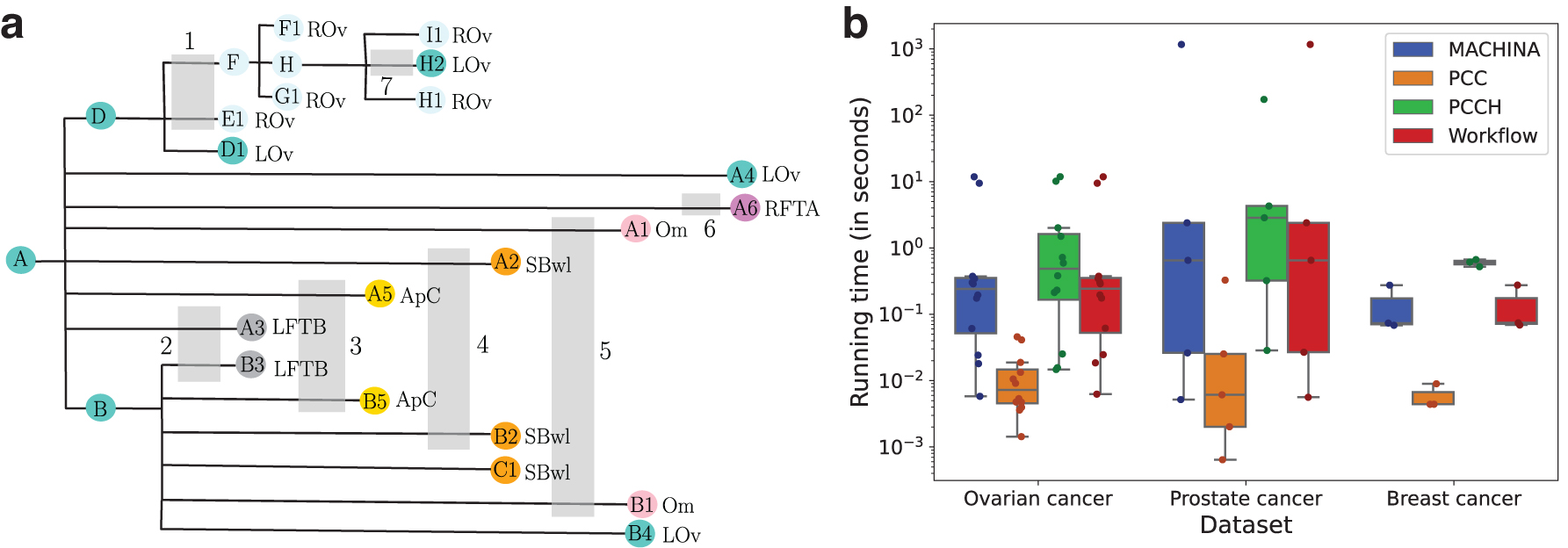
MACHINA and PCCH results for ovarian (McPherson et al., 2016), prostate (Gundem et al., 2015), and breast cancer (Hoadley et al., 2016) datasets. (a) PCCH results for ovarian cancer patient 1. Migrations enclosed within the same gray box represent a comigration (additionally labeled by timestamp) and vertex colors specify location labeling. (b) The running time (y-axis) for each method (color) across real datasets (x-axis).

We show the running time analysis for PCC, PCCH, MACHINA, and the workflow in Figure 7b and Supplementary Table S1. We found that PCCH generally takes slightly longer to finish (median of 0.474 seconds vs. 0.244 seconds for MACHINA). This is expected, as unlike MACHINA, PCCH includes checks for temporal consistency and returns timestamps along with a location labeling. Similar to the findings on simulated data, we found PCC to be significantly faster than PCCH or MACHINA. Since the MACHINA comigrations are temporally consistent, the workflow stops at step III, resulting in the running time of the workflow matching closely with that of MACHINA.

5.2.2. Prostate cancer

We ran PCCH and inferred the migration history of five androgen-deprived metastaic prostate cancer patients from Gundem et al. (2015). For the five selected patients, Gundem et al. (2015) sequenced both primary (prostate) and metastatic samples using whole-genome sequencing (WGS) technology. For each patient, they constructed a clone tree T by first identifying mutation clusters and calculating cancer cell fractions of each cluster in each sample by using an n-dimensional Bayesian Dirichlet process, and then inferring evolutionary relationships between pairs of mutation clusters by applying the “pigeon-hole” principle to mutation clusters within individual samples. To infer the migration histories, they deduced the location of origin of each mutation cluster by examining cancer cell fractions in each sample and using the “pigeon-hole” principle, and reported metastasis-to-metastasis migration in four (A10, A22, A31, and A32) out of five patients in consideration.

The samples from the same five patients were reanalyzed by MACHINA in El-Kebir et al. (2018), where it found simpler solutions with metastasis-to-metastasis spread only in two patients (A22, A32). MACHINA also did not report reseeding for any of the patients, which implies that the migration histories inferred by MACHINA are temporally consistent by Proposition 1. Indeed, we found that the inferred location labeling and the number of comigrations were identical for both PCCH and MACHINA. In terms of running times, we observed similar trends (Fig. 7b and Supplementary Table S2)—MACHINA was slightly faster than PCCH (median of 27.795 seconds vs. 0.67 seconds for MACHINA), although for patient A22, MACHINA (1702.24 seconds) needed more time than PCCH (185.18 seconds). For PCC, the running time was significantly shorter (median: 0.025 seconds). The workflow stops at step III because of $C_{M A C H I N A}$ being temporally consistent,

5.2.3. Breast cancer

We applied our methods to examine the migration history of two triple-negative breast cancer patients from Hoadley et al. (2016). DNA whole-genome sequencing was conducted on matched primary and multiple distant metastasis samples for both patients. The clonal structure was inferred using SciClone (Miller et al., 2014), and the phylogeny was determined using the ClonEvol R package (Dang et al., 2017). For patient A1, ClonEvol reported two potential clone trees due to its inability to accurately determine the evolutionary origin of clone 7. For patient A1, MACHINA recapitulated the findings reported in Hoadley et al. (2016) that all the clones except clones 6 and 9 originated in the primary location for both trees. For patient A7, MACHINA reported a parsimonious solution with eight migrations and six comigrations, and a comigration from primary location to lung for clones 2 and 4, which agreed with Hoadley et al. (2016).

All the results returned by MACHINA were temporally consistent, and so the workflow stopped at step III. Consequently, the migration histories inferred by MACHINA and PCCH were identical. Running times followed the same trend (Fig. 7b and Supplementary Table S3), with MACHINA being slightly faster than PCCH (median of 0.613 seconds vs. 0.074 seconds for MACHINA), and PCC being the fastest (median: 0.004 seconds).

6. CONCLUSION

In this article, we addressed a flaw in the definition of comigration adopted by MACHINA (El-Kebir et al., 2018). Specifically, we precisely defined spatial and temporal consistency for comigrations, leading to the formulation of three successive problems. The first problem, TCC, determines temporal consistency given a set of comigrations and derives a timestamp labeling for migrations in case the comigrations are temporally consistent. We showed that TCC can be solved in linear time. The second problem, PCC infers the smallest set of TCC given the locations of both leaf and internal vertices. We proved the problem to be NP-hard, indicating that even if the location of origin of every vertex and thus every migration is given as input, it is still computationally hard to deduce which migrations occurred simultaneously under a parsimony criterion.

Our third problem, PCCH, takes as input a leaf labeling, and infers the location labeling that minimizes the number of migrations, and subsequently the number of spatiotemporally consistent comigrations. We proved that PCCH is also NP-hard. In addition, we discussed MACHINA's views on comigrations and its limitations concerning temporal consistency and reported a sufficient condition under which MACHINA accurately computes comigrations. We presented ILP models for PCC and PCCH and proposed a workflow that combines the strengths of MACHINA, PCC, and PCCH—by using TCC to verify MACHINA's results and resorting to PCC and PCCH when needed. Finally, we conducted a comparative analysis of PCCH and MACHINA's performance on simulated and real data.

We generated simulation instances to investigate when MACHINA fails to determine temporally consistent comigrations and showed that MACHINA underestimates comigrations and may yield suboptimal location labeling in the presence of comigration graph cycles. For real data, PCCH returned the same location labeling as MACHINA for all instances.

PCCH offers several promising avenues for future research. While our current study focused on applying PCCH exclusively to cancer data, its versatility extends to inferring migration history in various organisms, including disease pathogens, as discussed earlier. Broadening the application of PCCH to diverse real datasets is crucial for gaining a comprehensive understanding of temporal inconsistency in practical scenarios. Drawing inspiration from MACHINA, which introduced parsimonious migration history with tree refinement, we plan to expand PCCH to incorporate tree refinement, aiming to minimize the number of migrations and comigrations lexicographically across all location labelings for possible tree refinements of the input tree. Furthermore, a captivating challenge lies in exploring the existence of multiple optimal solutions within the PCCH framework. Currently, PCCH provides a single optimal solution, yet, instances may arise where distinct location labelings yield the same number of migrations and TCC. Investigating the solution space within PCCH to detect and characterizing these alternatives represents a promising avenue for future research in this field.

Footnotes

ACKNOWLEDGMENTS

An earlier version of this article was published in WABI 2023 (doi: ). This project started as a collaboration at the Computational Genomics Summer Institute 2022.

AUTHORs' CONTRIBUTIONS

M.S.R.: Conceptualization, Implementation, Formal analysis, and Writing—Review. S.S.: Conceptualization and Writing—review. M.E.-K.: Conceptualization, Validation, and Writing—review and editing.

AUTHOR DISCLOSURE STATEMENT

The authors declare they have no conflicting financial interests.

FUNDING INFORMATION

Mohammed El-Kebir was supported by the National Science Foundation (CCF-2046488) as well as funding from the Cancer Center at Illinois. Sagi Snir was supported by the Israel Science Foundation (Grant No. ISF 1927/21) and the American/Israeli Binational Science Foundation (Grant No. BSF 2021139).

SUPPLEMENTARY MATERIAL

References

Aceto

, Bardia

, Miyamoto

, et al. Circulating tumor cell clusters are oligoclonal precursors of breast cancer metastasis. Cell, 2014; 158(5):1110–1122.

Birkbak

, McGranahan

. Cancer genome evolutionary trajectories in metastasis. Cancer Cell, 2020; 37(1):8–19.

Campbell

, Cori

, Ferguson

, Jombart

. Bayesian inference of transmission chains using timing of symptoms, pathogen genomes and contact data. PLoS Comput Biol, 2019; 15(3):e1006930.

Chauve

, Rafiey

, Davin

, et al. MaxTiC: Fast ranking of a phylogenetic tree by maximum time consistency with lateral gene transfers. bioRxiv, 2017; 2017:127548.

Cheung

, Ewald

. A collective route to metastasis: Seeding by tumor cell clusters. Science, 2016; 352(6282):167–169.

Cheung

, Padmanaban

, Silvestri

, et al. Polyclonal breast cancer metastases arise from collective dissemination of keratin 14-expressing tumor cell clusters. Proc Natl Acad Sci U S A, 2016; 113(7):E854–E863.

Comen

, Norton

, Massague

. Clinical implications of cancer self-seeding. Nat Rev Clin Oncol, 2011; 8(6):369–377.

Dadiani

, Kalchenko

, Yosepovich

, et al. Real-time imaging of lymphogenic metastasis in orthotopic human breast cancer. Cancer Res, 2006; 66(16):8037–8041.

Dang

, White

, Foltz

, et al. Clonevol: clonal ordering and visualization in cancer sequencing. Ann Oncol, 2017; 28(12):3076–3082.

10.

David

, Alm

. Rapid evolutionary innovation during an Archaean genetic expansion. Nature, 2011; 469(7328):93–96.

11.

Dellicour

, Baele

, Dudas

, et al. Phylodynamic assessment of intervention strategies for the West African Ebola virus outbreak. Nat Commun, 2018; 9(1):2222.

12.

El-Kebir

Parsimonious Migration History Problem: Complexity and Algorithms. In: 18th International Workshop on Algorithms in Bioinformatics (WABI 2018). Schloss Dagstuhl-Leibniz-Zentrum fuer Informatik: Germany; 2018.

13.

El-Kebir

, Satas

, Raphael

. Inferring parsimonious migration histories for metastatic cancers. Nat Genet, 2018; 50(5):718–726.

14.

Faries

, Steen

, Ye

, et al. Late recurrence in melanoma: Clinical implications of lost dormancy. J Am Coll Surg, 2013; 217(1):27–34.

15.

Faye

, Boëlle

P-Y

, Heleze

, et al. Chains of transmission and control of Ebola virus disease in Conakry, Guinea, in 2014: An observational study. Lancet Infect Dis, 2015; 15(3):320–326.

16.

Ferguson

, Donnelly

, Anderson

. Transmission intensity and impact of control policies on the foot and mouth epidemic in Great Britain. Nature, 2001; 413(6855):542–548.

17.

Gundem

, Van Loo

, Kremeyer

, et al. The evolutionary history of lethal metastatic prostate cancer. Nature, 2015; 520(7547):353–357.

18.

Hoadley

, Siegel

, Kanchi

, et al. Tumor evolution in two patients with basal-like breast cancer: A retrospective genomics study of multiple metastases. PLoS Med, 2016; 13(12):e1002174.

19.

Kahn

. Topological sorting of large networks. Commun ACM, 1962; 5(11):558–562.

20.

Kok

, Oshima

, Takahashi

, et al. Malignant subclone drives metastasis of genetically and phenotypically heterogenous cell clusters through fibrotic niche generation. Nat Commun, 2021; 12(1):863.

21.

Lafond

, Hellmuth

. Reconstruction of time-consistent species trees. Algorithms Mol Biol, 2020; 15(1):1–27.

22.

Libeskind-Hadas

, Charleston

. On the computational complexity of the reticulate cophylogeny reconstruction problem. J Comput Biol, 2009; 16(1):105–117.

23.

Maddipati

, Stanger

. Pancreatic cancer metastases harbor evidence of polyclonality. Cancer Discov, 2015; 5(10):1086–1097.

24.

Margeridon-Thermet

, Shulman

, Ahmed

, et al. Ultra-deep pyrosequencing of hepatitis B virus quasispecies from nucleoside and nucleotide reverse-transcriptase inhibitor (NRTI)–treated patients and nrti-naive patients. J Infect Dis, 2009; 199(9):1275–1285.

25.

Marrinucci

, Bethel

, Kolatkar

, et al. Fluid biopsy in patients with metastatic prostate, pancreatic and breast cancers. Phys Biol, 2012; 9(1):016003.

26.

McPherson

, Roth

, Laks

, et al. Divergent modes of clonal spread and intraperitoneal mixing in high-grade serous ovarian cancer. Nat Genet, 2016; 48(7):758–767.

27.

Merkle

, Middendorf

. Reconstruction of the cophylogenetic history of related phylogenetic trees with divergence timing information. Theory Biosci, 2005; 123:277–299.

28.

Miller

, White

, Dees

, et al. Sciclone: Inferring clonal architecture and tracking the spatial and temporal patterns of tumor evolution. PLoS Comput Biol, 2014; 10(8):e1003665.

29.

Nøjgaard

, Geiß

, Merkle

, et al. Time-consistent reconciliation maps and forbidden time travel. Algorithms Mol Biol, 2018; 13(1):1–17.

30.

Rambaut

, Posada

, Crandall

, et al. The causes and consequences of HIV evolution. Nat Rev Genet, 2004; 5(1):52–61.

31.

Räihä

K-J

, Ukkonen

. The shortest common supersequence problem over binary alphabet is NP-complete. Theor Comput Sci, 1981; 16(2):187–198; doi: 10.1016/0304-3975(81)90075-X

32.

Sanborn

, Chung

, Purdom

, et al. Phylogenetic analyses of melanoma reveal complex patterns of metastatic dissemination. Proc Natl Acad Sci U S A, 2015; 112(35):10995–11000.

33.

Sashittal

, El-Kebir

. SharpTNI: Counting and sampling parsimonious transmission networks under a weak bottleneck. bioRxiv, 2019; 2019:842237.

34.

Sashittal

, El-Kebir

. Sampling and summarizing transmission trees with multi-strain infections. Bioinformatics, 2020; 36(Suppl 1):i362–i370.

35.

Slatkin

, Maddison

. A cladistic measure of gene flow inferred from the phylogenies of alleles. Genetics, 1989; 123(3):603–613.

36.

Sobel Leonard

, Weissman

, Greenbaum

, et al. Transmission bottleneck size estimation from pathogen deep-sequencing data, with an application to human influenza A virus. J Virol, 2017; 91(14):e00171–17.

37.

Somarelli

, Ware

, Kostadinov

, et al. Phylooncology: Understanding cancer through phylogenetic analysis. Biochim Biophys Acta, 2017; 1867(2):101–108.

38.

Spada

, Sagliocca

, Sourdis

, et al. Use of the minimum spanning tree model for molecular epidemiological investigation of a nosocomial outbreak of hepatitis C virus infection. J Clin Microbiol, 2004; 42(9):4230–4236.

39.

Tabassum

, Polyak

. Tumorigenesis: It takes a village. Nat Rev Cancer, 2015; 15(8):473–483.

40.

Tofigh

, Hallett

, Lagergren

. Simultaneous identification of duplications and lateral gene transfers. IEEE/ACM Trans Comput Biol Bioinformatics, 2010; 8(2):517–535.

41.

Tonkin-Hill

, Martincorena

, Amato

, et al. Patterns of within-host genetic diversity in SARs-CoV-2. Elife, 2021; 10:e66857.

42.

Wang

, Sherrill-Mix

, Chang

, et al. Hepatitis C virus transmission bottlenecks analyzed by deep sequencing. J Virol, 2010; 840(12):6218–6228.

43.

Yamamoto

, Doak

, Cheung

. Orchestration of collective migration and metastasis by tumor cell clusters. Annu Rev Pathol, 2023; 18:231–256.

44.

, Bardia

, Wittner

, et al. Circulating breast tumor cells exhibit dynamic changes in epithelial and mesenchymal composition. Science, 2013; 339(6119):580–584.

Supplementary Material

Please find the following supplemental material available below.

For Open Access articles published under a Creative Commons License, all supplemental material carries the same license as the article it is associated with.

For non-Open Access articles published, all supplemental material carries a non-exclusive license, and permission requests for re-use of supplemental material or any part of supplemental material shall be sent directly to the copyright owner as specified in the copyright notice associated with the article.

0.00 MB

0.48 MB