Fuzzy-Based Identification of Transition Cells to Infer Cell Trajectory for Single-Cell Transcriptomics

Abstract

With the continuous evolution of single-cell RNA sequencing technology, it has become feasible to reconstruct cell development processes using computational methods. Trajectory inference is a crucial downstream analytical task that provides valuable insights into understanding cell cycle and differentiation. During cell development, cells exhibit both stable and transition states, which makes it challenging to accurately identify these cells. To address this challenge, we propose a novel single-cell trajectory inference method using fuzzy clustering, named scFCTI. By introducing fuzzy clustering and quantifying cell uncertainty, scFCTI can identify transition cells within unstable cell states. Moreover, scFCTI can obtain refined cell classification by characterizing different cell stages, which gain more accurate single-cell trajectory reconstruction containing transition paths. To validate the effectiveness of scFCTI, we conduct experiments on five real datasets and four different structure simulation datasets, comparing them with several state-of-the-art trajectory inference methods. The results demonstrate that scFCTI outperforms these methods by successfully identifying unstable cell clusters and obtaining more accurate cell paths with transition states. Especially the experimental results demonstrate that scFCTI can reconstruct the cell trajectory more precisely.

1. INTRODUCTION

Over the past decade, single-cell RNA sequencing (scRNA-seq) has emerged as a transformative technique, enabling the quantitative assessment of gene expression at the single-cell level. Given the intricate dynamics of cellular survival states, tracing the transcriptome profiles of individual cells remains a challenging task. However, by adopting measures to sample dynamic cells from a large number of cells, one can reconstruct the cellular developmental process from a computational perspective (Deconinck et al., 2021). Therefore, to capture the transitions in cell identity, branching differentiation processes, and asynchronous changes in biological function, one can use trajectory inference (TI) methods for computational modeling (Luecken and Theis, 2019). TI has emerged as a new subfield of computational biology, aimed at better understanding the potential dynamics of biological processes, such as cell development and immune response (Zhang et al., 2021).

Currently, many different methods have been developed for various datasets (Marco et al., 2014; Saelens et al., 2019; Chen et al., 2019). Cannoodt et al. (2016) proposed a unified framework to characterize TI methods, which is mainly divided into two parts: dimensionality reduction and trajectory modeling. Based on this framework, the recent TI methods can be grouped into two distinct categories. One is to make the cells within the trajectory more coherent through computational methods analyzing pseudo-time, exemplified by Slingshot (Street et al., 2018) and scTEP (Zhang et al., 2023). The other is centered around the development of innovative approaches to the dimensionality reduction step (Zhang et al., 2021).

The dimensionality reduction component involves techniques such as clustering. Data derived from scRNA-seq is complex and noisy, encompassing cells at various developmental stages and of different types. This complexity necessitates the use of clustering to effectively segregate data into groups corresponding to similar cell types or cell states, thereby establishing a strong foundation for subsequent trajectory reconstruction. Techniques such as PAGA (Wolf et al., 2019), TiC2D (Gan et al., 2022b), and scShaper (Smolander et al., 2022) focus on enhancing trajectory reconstruction through optimized clustering methods.

In reality, clustering methods can be divided into two types, distinguished by the way data is allocated to clusters. One is known as hard clustering, or discrete clustering (Pasin and Gonenc, 2023), where each cell is strictly assigned to a single cluster, leaving no room for ambiguity. A classical example of hard clustering is the Kmeans algorithm. Both TiC2D and scShaper are novel algorithms built on optimizing the typical Kmeans method. Kmeans is a classical clustering technique favored for its simplicity both conceptually and operationally, making it suitable for a wide range of data types. However, Kmeans is sensitive to the number of clusters specified and outliers. More critically, during cellular development, some cells transition from one stable state to another, rendering hard clustering like Kmeans inappropriate for such scenarios (Zheng et al., 2020).

Cells that exhibit unique but unstable cell states, and which are unsuitable for any specific cluster, can be termed fuzzy cells. While it is effective to identify cell critical states based on dynamical network biomarkers (Zhong et al., 2022, 2023), there is a scarcity of research focusing on optimizing clustering methods to study fuzzy cells and their trajectories. Existing hard clustering-based TI methods struggle to effectively identify these cells (Wang et al., 2022). Therefore, distinguishing cell types from a probabilistic or membership perspective is more meaningful for cells in unstable states (Kharchenko, 2021). DBCTI (Lan et al., 2022) and scTite (Gan et al., 2022a) are among the few TI algorithms that employ probabilistic clustering, utilizing probability distributions to identify fuzzy cells. Due to the minority of fuzzy cells in samples, methods such as scTite and DBCTI, which fit probability distributions, might lead to underfitting.

To address the aforementioned challenges, a TI method using single-cell fuzzy clustering (scFCTI) is proposed in this study. scFCTI is designed to identify fuzzy cell clusters representing transition states and subsequently infer accurate linear and branching trajectories from scRNA-seq data. Initially, scFCTI applies the fuzzy clustering method (Ruspini, 1970) to segment cells into distinct subgroups that represent various cellular states. Subsequently, a novel metric, termed fuzzy transition entropy, is introduced to identify cells displaying unstable states. These identified fuzzy cells are then directionally filtered, and a new fuzzy cell cluster is defined between each pair of stable cellular states to obtain a refined set of cell clusters. Correspondingly, scFCTI leverages the Minimum Spanning Tree (MST) algorithm to infer the developmental paths of both stable and fuzzy cells. Ultimately, the pseudo-time of cells is calculated through the principal curve algorithm to obtain a cell trajectory with predicted pseudo-time.

To substantiate the superiority, scFCTI is evaluated on four types of simulated datasets with varying structures and five real datasets with known lineages. scFCTI successfully reconstructs more accurate cellular trajectories with transition paths. The comparison with state-of-the-art methods shows that the fuzzy clustering approach indeed enhances the efficiency of TI.

2. METHODS

2.1. Datasets and data preprocessing

To further demonstrate the effectiveness of scFCTI in inferring single-cell trajectories, we apply the method to five real scRNA-seq datasets and four simulation datasets with different structures.

The first dataset, HSMM (Trapnell et al., 2014), contains 372 single cells and 2201 genes collected from primary human skeletal muscle myoblasts at 0, 24, 48, and 72 hours. The second dataset consists of scRNA-seq samples collected from bone marrow-derived mouse dendritic cells stimulated with lipopolysaccharide, LPS (Amit et al., 2009), at 1, 2, 4, and 6 hours, consisting of 306 cells and 8215 genes. The third dataset comprises scRNA-seq samples from quiescent neural stem cells, qNSC (Shin et al., 2015), in the hippocampus, including 172 cells and 5014 genes collected from the same cell population. The fourth dataset, hESC (Leng et al., 2015), is obtained by sequencing 460 human embryonic stem cells and 12,423 genes, including 213 H1 single cells and 247 H1-Fucci single cells. Furthermore, we apply scFCTI to a hematopoiesis dataset which primarily describes the differentiation between hematopoietic stem cell (HSC) and hematopoietic progenitor cell populations, HEMA, encompassing 1428 cells and 8422 genes (Kowalczyk et al., 2015). The five datasets are referred to as HSMM, LPS, qNSC, hESC, and HEMA, respectively.

We use dyngen, a multimodal simulation engine for studying dynamic cellular processes at a single-cell resolution (Cannoodt et al., 2021), to generate simulated data for testing the effectiveness of scFCTI. Different simulated datasets are obtained by setting linear, bifurcating, cycletree, and multicycle trajectory backbones. The simulated datasets provide the ground truth of time which can be used as a gold standard for comparison with the predicted pseudo-time.

Due to the inherent limitations of single-cell sequencing, such as sparsity and dropouts (Hicks et al., 2018), a series of preprocessing steps are applied to the datasets. These include gene filtering, normalization, and square-root transformation. Specifically, scFCTI perform a filtering step to remove genes with no expression, followed by a gene selection step to retain genes expressed in over one-third of the cells. As dropouts in single-cell sequencing are a common issue, the MAGIC method (van et al., 2018) is employed to address this problem.

To highlight the effectiveness of the MAGIC method, we conduct a comparative analysis of 2D and 3D visualization and clustering results of recovered and unrecovered data. The specific results of the comparison can be found in Supplementary Figs. S1 and S2. The results clearly demonstrate that the MAGIC method significantly improves the completeness of the trajectory changes in the datasets. In addition, to avoid the issue of the curse of dimensionality in subsequent calculations, scFCTI utilizes principal component analysis (PCA) (Ringnér, 2008) to obtain a low-dimensional representation of the data.

2.2. The overview of scFCTI

To reconstruct cell trajectories from scRNA-seq data, we propose a novel single-cell TI method called scFCTI. scFCTI utilizes fuzzy clustering to identify fuzzy cells and stable-state cells by introducing the concept of fuzzy transition entropy. Based on the different states of cells, scFCTI constructs an MST based on cell clusters. scFCTI consists of four main steps: cell clustering based on membership degree, identification of fuzzy cells using fuzzy transition entropy, TI, and pseudo-time calculation, as illustrated in Figure 1. The detailed descriptions of these steps are presented in the following sections.

FIG. 1.

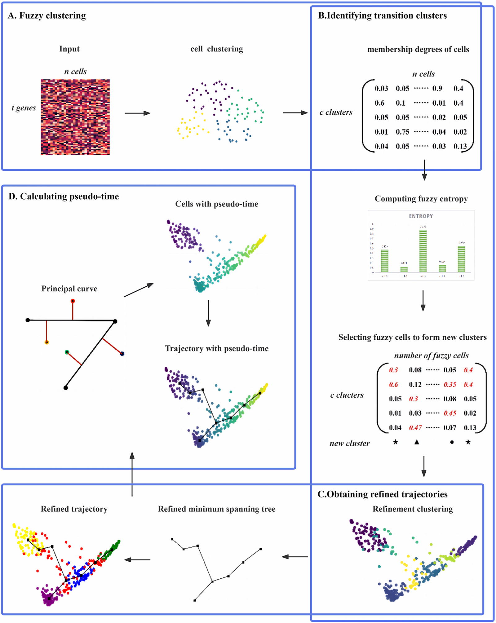
The overview of scFCTI. (A) Employ the fuzzy clustering method to cluster cells. (B) Compute the fuzzy transition entropy of each cell and selectively filtering fuzzy cells as transition cells. (C) Construct the MST for the refined cluster to derive the cell trajectory. (D) Apply the principal curve algorithm to calculate the pseudo-time of cells, thus obtaining the final cell trajectory. scFCTI, single-cell fuzzy clustering.

2.2.1. Performing fuzzy clustering on single cells

The input to the scFCTI algorithm is a preprocessed gene expression matrix with t genes and n cells X_t×n , where each element in the matrix represents the expression level of gene i in cell j. To facilitate a more insightful and efficient understanding of the data, PCA is employed to reduce the dimensionality of the matrix and obtain a low-dimensional representation of the data.

In order to infer more accurate cell trajectories, we first perform cell clustering. Due to the fuzzy cells, intermediate or uncertain phenotypic states are difficult to assign to a single cluster. To this end, scFCTI adopt the fuzzy c-means (FCM) clustering method, which is a soft clustering. When using FCM clustering, cells can be assigned to two or more clusters based on the various membership degrees that they exhibit. Unlike traditional hard clustering methods, which require cells to be unambiguously assigned to a single cluster, FCM clustering allows for greater flexibility and more organic clustering boundaries.

It calculates the membership degree of each cell to each cluster. In other words, each cell is assigned a certain membership degree to each cluster, rather than being definitively assigned to a single cluster. Similar to probability, the sum of membership degrees of each cell to all clusters is equal to 1. To achieve optimal fuzzy partitioning, the following function is minimized: $J = \sum_{i = 1}^{c} \sum_{j = 1}^{n} u_{i j}^{m} {‖ x_{j} - C_{i} ‖}^{2}, \sum_{i = 1}^{c} u_{i j} = 1,$ (1)where c represents the number of categories. Correspondingly, there are c centers C_i, where i = 1, 2, …, c. Each individual cell is represented by x_j, where j = 1, 2, …, n. The membership degree of each cell is represented as u_ij. The degree factor is m, which ranges from 1.5 to 2.5.

Subsequently, we aim to compute the minimum value of the objective function J in order to obtain the membership degree matrix U_ij. To facilitate the calculation, we utilize the Lagrange multiplier method to solve the objective function: $L (x, λ) = \sum_{i = 1}^{c} \sum_{j = 1}^{n} u_{i j}^{m} {‖ x_{j} - C_{i} ‖}^{2} + λ_{1} (\sum_{i = 1}^{c} u_{i 1} - 1) + λ_{2} (\sum_{i = 1}^{c} u_{i 2} - 1) + \cdot \cdot \cdot + λ_{j} (\sum_{i = 1}^{c} u_{i j} - 1) + \cdot \cdot \cdot + λ_{n} (\sum_{i = 1}^{c} u_{i n} - 1) .$ (2)

It can be simplified into the following form: $L (x, λ) = J + \sum_{i = 1}^{c} λ_{i} h_{i} (x),$ (3)where $h_{i} (x) = \sum_{i = 1}^{c} u_{i j} - 1,$ (4)where λ is a constant weight, its value lies within the range of [0,1].

Next, following the general steps of the Lagrange multiplier method, we derive the derivatives of u_ij and C_i respectively: $\frac{\partial J}{\partial u_{i j}} = m {‖ x_{j} - C_{i} ‖}^{2} u_{i j - 1}^{m} + λ_{j} = 0,$ (5) $\frac{\partial J}{\partial C_{i}} = \sum_{j = 1}^{n} [- u_{i j}^{m} \cdot 2 \cdot (x_{j} - x_{i})] .$ (6)

The iterative formula can be obtained as follows: $u_{i j} = \frac{1}{\sum_{k = 1}^{c} {(\frac{‖ x_{j} - C_{i} ‖}{‖ x_{j} - C_{k} ‖})}^{\frac{2}{m - 1}}},$ (7) $C_{i} = \frac{\sum_{j = 1}^{n} u_{i j}^{m} \cdot x_{j}}{\sum_{j = 1}^{n} u_{i j}^{m}} .$ (8)

From the formula above, it can be clearly observed that u_ij and C_i are interrelated. Finally, by setting the maximum iteration number p, the above equation is iteratively optimized to determine the output membership matrix, cluster centers, and other relevant values. According to the maximum membership degree belonging to a specific cluster, these cells are assigned to different clusters while maintaining their different membership degree values for different clusters.

2.2.2. Utilizing fuzzy transition entropy to identify fuzzy cells

After fuzzy clustering, we obtain a membership matrix U_ij in which each element u_ij represents the membership degree of each cell to each cluster. From the membership degree matrix, it can be observed that the majority of cells have high membership degrees for a specific cluster, indicating that these cells are in a stable state and strictly belong to that cluster. Conversely, a small proportion of cells have comparable membership degrees for multiple clusters, suggesting that these cells may have functional significance in multiple clusters. Thus, the membership degree matrix provides an intuitive way to distinguish between fuzzy and stable cells.

To quantitatively distinguish between the two aforementioned cell states, we introduce a new metric called single-cell fuzzy transition entropy, using the membership degrees that have already been calculated. Similar to Shannon entropy, this metric is defined as follows: $H (j) = \sum_{i = 1}^{c} \sum_{j = 1}^{n} u_{i j} \log (u_{i j}),$ (9)where u_ij is the membership degree of every cell x_j ∈ C _i , c denotes the number of cell clusters, and H(j) represents the fuzzy transition entropy of cell j. As a result of the properties of entropy, cells with higher values of fuzzy transition entropy are more likely to exhibit similar membership degrees in multiple clusters. While the cells with lower values are more likely to be in a stable state.

The fuzzy cells that have been selected above are considered as transition states between two stable cellular states. Then it is important to distinguish which transition cluster these fuzzy cells belong to. We compare their membership degrees and select the two original cell clusters with the highest membership degree values. Naturally, the fuzzy cells are considered as transition cells between these two cell clusters. However, it is worth noting that these transition clusters do not indicate the emergence of new cell types, but rather a reclassification of a group of preexisting cells with unstable gene expression patterns.

2.2.3. Constructing the initial and refined MST

After performing the above steps, a series of basic cell clusters and refined cell clusters are available. To establish the initial structure of cell trajectories, scFCTI employs the MST algorithm. First, the primary cell clusters are utilized as input to generate an undirected connected graph, from which a subgraph in the form of a tree is generated. Each node in the tree represents a cluster center, and the length of each edge in the graph is represented by the Euclidean distance between the connecting nodes. The MST is defined as the tree with the smallest total edge length among all possible spanning trees. Combined with previous research, it is preferred to use the Kruskal algorithm to determine the connected edges and basic cell development path. In the absence of any prior information, the Kruskal algorithm randomly selects a node as the origin of the path and iteratively optimizes to determine the initial MST.

Subsequently, the refined cell clusters are used as new input to obtain a refined MST using the same procedure, as shown in Figure 1C.

Algorithm 1: Kruskal’s Algorithm for Generating MSTInput: An undirected connected graph with f nodes G = (V_G, E_G), a set of edge weights D = (d_ij), where d_ij represents the Euclidean distance between cluster i and cluster j.Output: the MST 1: Initialize an empty MST and an empty set of edges E2: For each node in the graph v $\in$ V_G, add it as an independent set to a list of sets C3: For each edge in the graph e $\in$ E_G, add it to the set of edges E4: Sort E in ascending order of edge weight.5: For each edge e $\in$ E, execute the following steps:5.1: If both endpoints of the edge e are in the same set, discard the edge to prevent cycle formation.5.2: Otherwise, add the edge e to the MST and merge the sets containing the two endpoints of the edge e into a single set.6: Return the MST.

2.2.4. Calculating pseudo-time and obtaining refined cell trajectories

Before calculating the pseudo-time of each cell, it is essential to determine the starting point of the trajectory, namely, the initial cell cluster. It has been found that in the early stages of development, cells exhibit similar expression patterns due to the sharing of many genes (Dong et al., 2018). For example, most cells in the early stages of embryonic development demonstrate a high degree of similarity. In other words, cells located at local developmental endpoints represent highly heterogeneous mature cells. Accordingly, leveraging this trait, we introduce shared nearest neighbors (sNN) to quantify the similarity of the r-th cluster: $sNN (x, y) = | N (x) \cap N (y) |,$ (10)where x, y $\in$ cluster represent any two cells, N(x), N(y) represent their respective neighboring nodes. | · | means the size of the set, sNN(x,y) indicates the number of common neighbors between nodes x and y. Afterward, the similarity between each cell and its sNN is computed, which yields the mean similarity of sNN for each cluster.

In accordance with the research objective of this article, the principal curve algorithm is ultimately chosen to determine the pseudo-time of cells, which is implemented in Python using the princurve package. Specifically, all cells are projected onto the nearest path, and the distance from the starting point of the curve to each projected point is calculated to derive the pseudo-time ordering of the cells.

Algorithm 2: The sNN algorithm for acquiring the sNN of cells within a clusterInput: A cluster of cellsOutput: A similarity matrix for the cluster of cells 1: Find the r-nearest neighbors for each cell in the cluster.2: If neither cell x nor y is among the r-nearest neighbors of the other within the cluster then3: similarity(x,y) ← 04: else5: similarity(x,y) ← the number of shared nearest neighbors6: end if

2.2.5. Other methods for dimensionality reduction and parameter determination

PCA is the dimensionality reduction method used in this study, which is a widely used dimensionality reduction method (Wolf et al., 2019; Street et al., 2018). Other methods such as UMAP (Becht et al., 2018), t-SNE (Kobak and Berens, 2019), and PHATE (Moon et al., 2019) are also considered. We currently employ four different dimensionality reduction methods on five distinct datasets, as depicted in Supplementary Fig. S3. PCA demonstrates superior performance on these datasets. Furthermore, we conduct subsequent trajectory analysis of PCA and the other three methods on the datasets, illustrated in Supplementary Fig. S4.

During the process of fuzzy clustering, the membership degree factor, denoted as m, is typically set to 2. This value is widely used as it offers a balance between cluster separation and fuzziness, applicable for a broad range of datasets. In order to further study the influence of m, we have carried out robustness experiments on m, as shown in Supplementary Fig. S5. Set the m range to 1.5–2 and apply it to five real datasets. Adjusted Rand Index (ARI) is used as the evaluation criterion. Although with the change of m, the performance does vary. But if we observe carefully, the change of the results is not obvious. On the other hand, fuzzy clustering is an unsupervised clustering method that determines the optimal number of clusters by comparing the values of fuzzy partition coefficient (fpc). The iteration number, p, is usually set to 100, as taking a higher value may result in a longer runtime and poorer calculation outcomes.

The determination of the fuzzy transition entropy threshold is guided by the distinctive characteristics of each dataset. Also, the threshold value is chosen by considering the impact of newly formed clusters consisting of fuzzy cells on the subsequent trajectory generation. Meanwhile, it is worth noting that changes in the threshold value do not fundamentally alter the existence of transition states between clusters. Specifically, two clusters without transition states do not generate transition clusters as the threshold decreases continuously. Last, but not least, when calculating the intracluster similarity using the sNN algorithm, the nearest-neighbor number k is typically set within the range of [5,10], with a default value of k = 5.

On the basis of the parameter settings of scFCTI, we calculate the computational complexity of scFCTI. Given the size of the dataset, the computational complexity of scFCTI is O(iCp), where i represents the number of cells, C represents the number of clusters, and p represents the number of iterations involved.

3. RESULTS

3.1. TI for real single-cell datasets

To evaluate the ability and effectiveness of scFCTI in inferring cell trajectories, we apply it to five widely used scRNA-seq datasets, HSMM, LPS, qNSC, hESC, and HEMA, which are generated using different sequencing technologies in different environments. First, scFCTI clusters cells into different subgroups using the fuzzy clustering approach. Secondly, a new measure is introduced, fuzzy transition entropy, to identify fuzzy cells as transition cells. Then, we obtain cell paths by refining the basic clusters and adding transition cells. Before cell sorting, scFCTI uses the sNN to quantify the similarity of clusters. At last, scFCTI calculates the pseudo-time of cells using the principal curve algorithm to derive a cell trajectory with pseudo-time. The reconstructed cell trajectories of these five real datasets are shown in Figure 2.

FIG. 2.

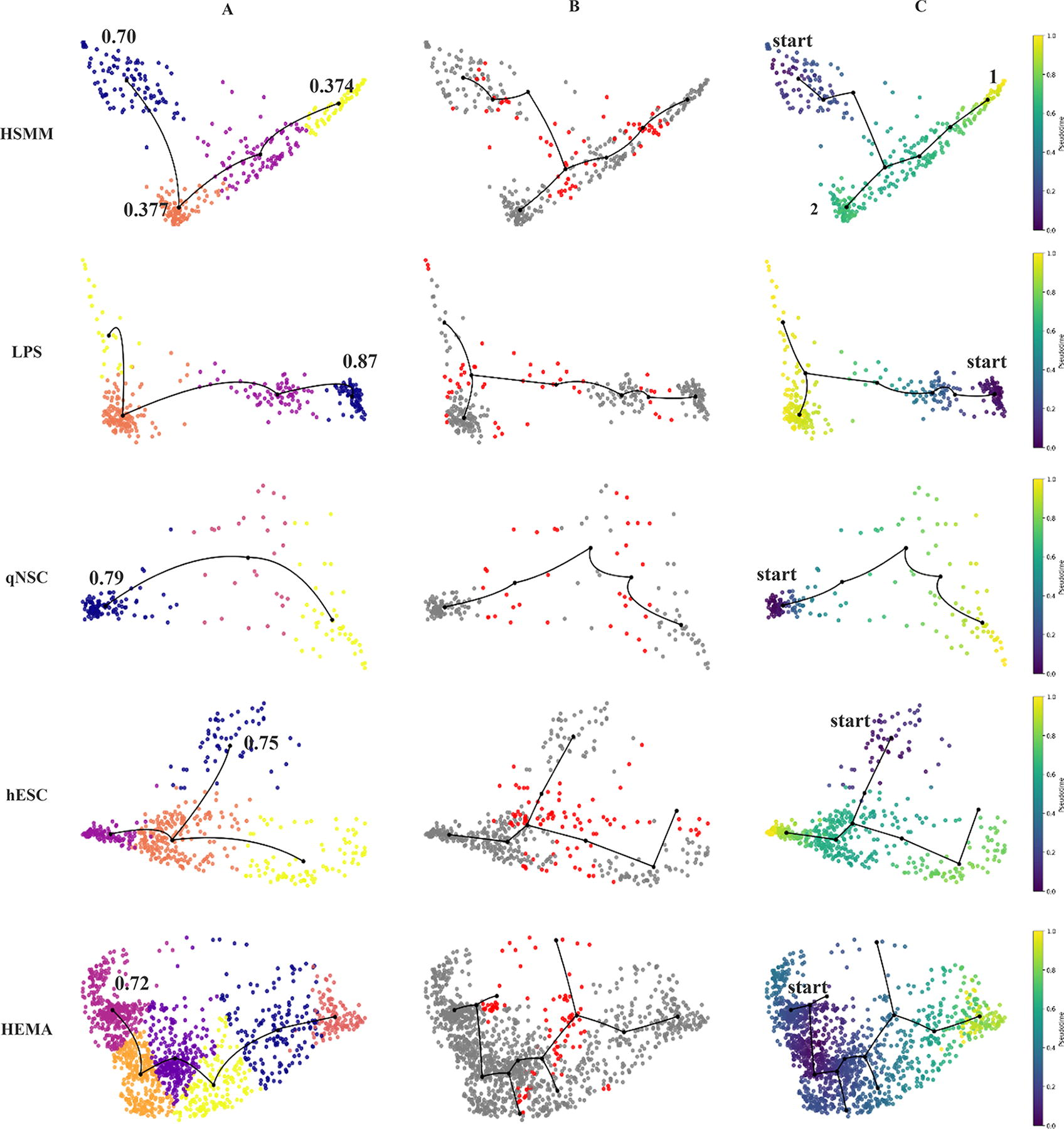
scFCTI reconstructs the trajectory and pseudo-time for five real scRNA-seq datasets (HSMM, LPS, qNSC, hESC, and HEMA). (A) Depict the cell trajectory obtained based only on the generated fundamental clusters. (B) Illustrate the refined cell trajectory generated by introducing the identified transition cell clusters. The red points represent transition cells. (C) Present the final cell trajectory formed with pseudo-time. The darker the color of the cell, the closer it is to a starting point. LPS, lipopolysaccharide; qNSC, quiescent neural stem cells.

By means of fuzzy clustering and MST, as shown in Figure 2A, we can obtain the fundamental developmental paths of cells, which generally contain only one main path. By incorporating the identified transition cells based on the defined fuzzy transition entropy, it is evidently observed that the position of the transition cells on the given trajectory calculated by scFCTI, shown in red (Fig. 2B). These cells are basically at the turning point of their trajectories, which further confirms the significance of the existence of transition cells. Based on these transition cells, the cell trajectory contains not only the main path but also refined branching paths.

Regarding the HSMM dataset, previous studies have indicated the presence of contaminated stromal mesenchymal cells in the dataset (Fig. 3A). Specifically, the start→2 path represents the contaminated cells, while the start→1 path means the main differentiation path (Fig. 3B). However, in the TiC2D (Fig. 3C), only one differentiation path is constructed for the HSMM dataset without excluding the contaminated cells, which is deemed suboptimal. This may be attributed to the fact that the consensus clustering method used in the TiC2D method has already treated the contaminated cells as effective cells. In this article, scFCTI initially identifies four clusters that mainly correspond to the cell groups collected at 0, 24, 48, and 72 hours. The maximum sNN similarity value for the initial cluster is determined to be 0.7, which further confirms the consistency of cell trajectory reconstruction for the HSMM dataset with previous research. Additionally, the contaminated cells are found not to participate in the primary cell development, as shown by the pseudo-time values (Fig. 3B, left).

FIG. 3.

scFCTI reconstructs the trajectory and pseudo-time for the dataset HSMM. (A) Ground truth from Trapnell et al. (2014) experiment results on the HSMM dataset, with the contaminated cells marked in green. (B) Visualization of scFCTI’s result on the HSMM dataset. The red points represent transition cells. The signs “1” and “2” represent two branches, respectively. (C) Visualization of TiC2D’s (Gan et al., 2022b) result on the HSMM dataset. (D) Ground truth of key factor MEF2C in original dataset with four moments. (E) Expression levels of key factor MEF2C in all clusters, which is derived from scFCTI. (F) Visualization of scFCTI’s result on the HSMM dataset, including the initial and transition clusters. Different colors indicate different clusters.

Skeletal muscle cells are multinucleated cells formed by fusion of myogenic cells. In particular, we confirm the validity of the existence of transition clusters by verifying the performance of MEF2C. Myocyte enhancer factor 2 (MEF2) is a TF family, which plays an important role in the myogenesis of skeletal muscle and is crucial for muscle differentiation (Jin et al., 2017). We examine the expression of MEF2C in the original dataset by means of a violin diagram, and the results detected at four different times are shown in Figure 3D. It can be observed that the initial expression of MEF2C is relatively stable, indicating that myogenic differentiation and proliferation have not yet started. However, the expression of MEF2C is significantly upregulated at 24 and 48 hours, indicating the initiation of myogenic proliferation to prepare for the subsequent fusion of skeletal muscle cells. Based on this, we further check the expression of MEF2C in all clusters obtained by using the scFCTI method, including transition clusters (Fig. 3E).

The first four clusters generated by scFCTI correspond to the original authentic clusters, whereas the subsequent four represent latent transition clusters (Fig. 3F). According to our definition, cluster 4 is the transition cluster from 0 to 24 hours, which means that it contains all transition cells from 0 to 24 hours. According to the violin plot, the expression of MEF2C in cluster 4 shows a transition from low to high. This is consistent with the experimental results of Trapnell et al. (2014).

For the LPS dataset, scFCTI identifies four clusters corresponding to the cell groups collected at 1, 2, 4, and 6 hours after lipopolysaccharide stimulation of bone marrow-derived dendritic cells. The initial MST has only one main path. Upon using sNN to identify the starting clusters and adding the positions of fuzzy cells, it becomes evident that there are two branching paths. The resulting sNN similarity values of the four identified clusters are 0.23, 0.26, 0.14, and 0.87. The latter cluster serves as the origin of the pseudo-time trajectory, which is consistent with previous experimental results (Fig. 2, LPS). For the qNSC dataset, it has three clusters but no multiple time points or experimental conditions. The basic structure of qNSC can be obtained by using scFCTI. Finally, a cell trajectory showing two branching paths is obtained (Fig. 2, qNSC).

For the hESC dataset, while the MST structure generated based on the initial clusters already indicates branching trajectories, we clearly visualize the transition path of cells from one stable state to another by fuzzy cells marked in red. In addition, scFCTI is also applied to hematopoietic cells. This dataset focuses on the relationship between hematopoietic stem cells and hematopoietic progenitor cell populations. By comparing the ground truth and reconstruction result (Fig. 4A, C), scFCTI successfully captures the original cell development structure. In addition, with the help of transition cells, we reconstruct subsequent developmental trajectories, which is not achieved by the DBCTI approach (Fig. 4B).

FIG. 4.

scFCTI reconstructs the trajectory and pseudo-time for the dataset HEMA. (A) Ground truth from Kowalczyk et al. (2015) experiment results on the HEMA dataset. (B) Visualization of DBCTI’s (Lan et al., 2022) results on the HEMA dataset. (C) Visualization of scFCTI’s result on the HEMA dataset. The red points represent transition cells.

3.2. Gene expression analysis of transition cells

In addition, to comprehensively understand the intricacies of the cell development process, we conduct a study on the importance of fuzzy cells and fuzzy cell clusters within cell trajectories. As previously mentioned, fuzzy cells primarily exhibit similar membership degrees to two or more clusters. By employing scFCTI, we amalgamate fuzzy cells with similar membership degrees into new sets, as fuzzy cell clusters. It is important to note that these fuzzy cell clusters do not represent novel cell types. In fact, they denote transition states between two stable cell states and can be considered as transition cells. Therefore, by analyzing the gene expression patterns of transition cells, one can further elucidate the critical role of transition cells in the developmental progression of cell trajectories.

In order to quantify the selection of specific genes, we use coefficient of gene variation (CV_gene) as a computational rationale. CV_gene is a statistic used to measure the degree of expression variation in gene expression data. The calculation formula is as follows: $C V_{gene} = \frac{σ}{μ},$ (11)where σ represents the standard deviation of gene expression levels, μ represents the mean value of gene expression level. Based on the CV_gene values of each dataset, we select the genes in Table 1 for further study.

Table 1.

The Rankings of Genes Used for Further Analysis

Datasets	Genes	Rankings	Total number of genes
HSMM	LINC03033	78	2201
HSMM	MEF2C	79	2201
LPS	PPARGC1B	2	8215
LPS	IFI44	59	8215
qNSC	Neurod1	13	5014
qNSC	Sox11	18	5014
hESC	GNA14	1	12,423
hESC	TUBB8	5	12,423
HEMA	Cdkn3	1	8422
HEMA	Nusap1	7	8422

LPS, lipopolysaccharide; qNSC, quiescent neural stem cells.

The HSMM dataset is related to skeletal muscle cell formation, which is achieved by the fusion of fibroblasts and myogenic cells. We find in our results a gene LINC03033, which is a noncoding RNA related to fibroblasts and is a member of the LncRNA-CAF family (Ding et al., 2018). In cells collected at time 0 hour, there are more fibroblasts, indicating an early stage of skeletal muscle cell development (Fig. 5A). At the period of 0 hour→48 hours, the expression of LINC03033 decreases significantly, which means fibroblasts begin to transform into myoblasts. This is consistent with the expression of transition cluster 7 between clusters 24 and 48 hours, generated by scFCTI (Fig. 5B). For further verification, we characterize the continuous expression of LINC03033 in transition cluster 7 (Fig. 5C). Obviously, the line chart shows a significant downward pattern (Fig. 5D). After screening the top 50 variable genes, we also generate the gene expression heatmap for datasets HSMM and LPS (Supplementary Fig. S6).

FIG. 5.

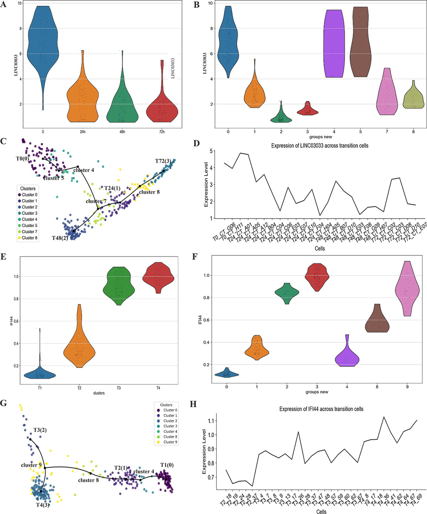
The gene expression analysis for the datasets HSMM and LPS. (A) Ground truth of key factor LINC03033 in original dataset with four moments. (B) Expression levels of key factor LINC03033 in all clusters, which is derived from scFCTI. (C) Visualization of scFCTI’s result on the HSMM dataset, including the initial and transition clusters. Different colors indicate different clusters. All four time points have been marked, and the numbers in brackets represent the index of that time point in all clusters of scFCTI. (D) Expression levels of key factor LINC03033 in transition cluster 7 between 24 (cluster 1) and 48 hours (cluster 2). (E) Ground truth of key factor IFI44 in original dataset with four states. (F) Expression levels of key factor IFI44 in all clusters, which is derived from scFCTI. (G) Visualization of scFCTI’s result on the LPS dataset, including the initial and transition clusters. Different colors indicate different clusters. All four states have been marked, and the numbers in brackets represent the index of that time point in all clusters of scFCTI. (H) Expression levels of key factor IFI44 in transition cluster 8 between T2 (cluster 1) and T4 (cluster 3).

The LPS dataset mainly concerns the degree of maturation of dendritic cells stimulated by lipopolysaccharide. When it comes to dendritic cells, IFI144 is discovered as a shared biomarker and disease target for coronavirus disease 2019 (COVID-19) (Zheng et al., 2022).

Through further research, IFI44 is actually an interferon-induced protein that expresses antiproliferative factors that have no effect on respiratory syncytial virus (RSV) attachment but reduce RSV replication in a minigenome assay (Busse et al., 2020). It has been observed that the expression levels of genes related to interferon-induced proteins, such as IFI44, are low in cells collected after the first two stimulations and significantly increase in cells collected after the subsequent two LPS stimulations (Fig. 5E). The first four clusters generated by scFCTI correspond to the original clusters, whereas the subsequent three represent potential transition clusters (Fig. 5G). Then, we quantify the expression of IFI44 in transition cluster 8, between T2 and T4. Whether it is a violin chart (Fig. 5F) or a line chart (Fig. 5H), IFI44 shows a transition from low to high in transition cluster 8. This is consistent with the expression level transition from T2→T4 in the original data. Also, it further confirms that the information carried by the original data is not lost after using MAGIC.

Regarding HEMA dataset, a rare population of multipotent HSC cells is required for the continuous production of millions of mature blood cells while maintaining a correct balance between the different lineages. At the same time, in multipotent progenitors (MPP), expression variability is largely independent of age. We obtain a consistent conclusion by visualizing the 20 genes with high CV_gene values (Fig. 6A, B). After conducting experiments, one can find that Cdkn3 prevents premature G1/S transition by dephosphorylating interphase cyclin-dependent kinases to prevent premature inactivation of the RB pathway (Sun et al., 2016), as shown in Figure 6C. It is pertinent to note that the first six clusters generated by scFCTI correspond directly to the original true clusters, whereas the subsequent seven clusters represent potential transition states (Fig. 6D). Through the annotation information, cluster 17 is a transition cluster from HSC to MPP. Likewise, it can be observed that the expression in transition clusters (Fig. 6E). This further confirms the effectiveness of scFCTI.

FIG. 6.

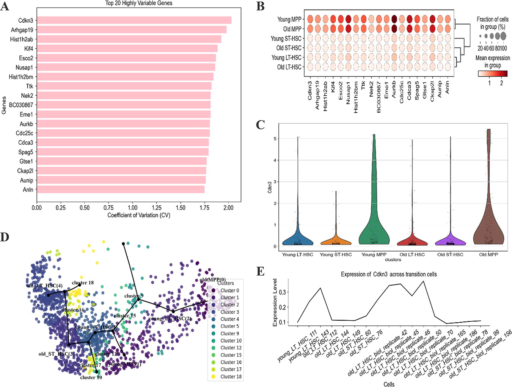
Performance of specific genes in HEMA. (A) Ranking bar chart of the top 20 genes ranked from high to low coefficient of variation. (B) Dot plot of the top 20 genes within 6 populations. (C) Expression levels of key factor Cdkn3 in original clusters. (D) Visualization of scFCTI’s result on the HEMA dataset, including the initial and transition clusters. Different colors indicate different clusters. (E) Expression levels of key factor Cdkn3 in transition clusters 17 between young_LT_HSC (clusters 3) and old_LT_HSC (cluster 5).

Through our study of transition cells, it can be demonstrated that once again these cells in transition states exhibit significant differences from their stable-state counterparts. Furthermore, it has been shown that cells within transition clusters are of particular interest, as they bridge the gap between two separate clusters and express genes in a manner that is markedly distinct from stable cells within other clusters.

As such, the scFCTI method is based on refined cell clusters and is capable of constructing trajectories that more accurately reflect the original developmental path of cells. The above research also fully demonstrates that these fuzzy cells play an irreplaceable role in the process of reconstructing cell trajectories. There are additional visualizations of transition cells in other datasets (Supplementary Figs. S6, S7, S8 and S9). Similarly, in these supplementary visualization figures, there is usually a large fluctuation in the expression of these genes in the transition cluster. This further demonstrates the significance of the existence of transition cells. In particular, there is actually no direct developmental relationship between time points C and R (Supplementary Fig. S7D). In scFCTI’s result, there is indeed no transition cluster generated between C and R, which further confirms the accuracy of scFCTI.

3.3. Comparison of methods

In order to assess the accuracy of our method, we utilize ARI, Normalized Mutual Information (NMI), and ACCuracy (ACC) as measures to evaluate the performance. ARI, as a clustering evaluation metric, calculates the degree of similarity between the real results and the clustering results by computing the number of cells that belong to the same or different clusters. ARI is calculated as follows: $ARI = \frac{2 (ε_{s s} - ε_{s q})}{(ε_{s s} + ε_{s q}) (ε_{s q} + ε_{q q}) + (ε_{s s} + ε_{q s}) (ε_{q s} + ε_{q q})},$ (12)where ε_ss represents the number of cells that belong to the same clusters in both the actual and inferred scenarios, ε_sq represents the number of cells that are in the same clusters in the actual scenario but in different clusters in the inferred scenario, ε_qs represents the number of cells that are in different clusters in the actual scenario but in the same clusters in the inferred scenario, and ε_qq represents the number of cells that are in different clusters in both the actual and inferred scenarios. The range of ARI values is [−1,1]. The closer the calculated value is to 1, the better the clustering performance is.

ACC is a metric to test whether the classification is correct or not, which calculates the proportion of cells correctly classified in the clustering results to the total number of cells. This metric only considers whether the sample classification is correct, without taking into account the precision and recall of the classification. ACC is calculated as follows: $ACC = \frac{n_{i i}}{n},$ (13)where n_ii represents the number of correctly classified samples in the i-th class of the clustering results, and n represents the total number of samples. The range of ACC values is [0,1]. A higher value of ACC indicates a better clustering performance.

To further demonstrate the effectiveness of scFCTI, we have incorporated the use of NMI as an additional evaluation criterion. NMI is a widely used metric for assessing the similarity between clustering results and known labels. It quantifies the similarity value between 0 and 1 when comparing two clustering results. One advantage of NMI is that it is not influenced by the ordering of labels, unlike the ACC metric. The calculation of NMI can be expressed as follows: $NMI (Y, C) = \frac{2 \times I (Y, C)}{C E (Y) + C E (C)},$ (14)where Y represents the true labels of the data, C represents the results of clustering, and CE(·) represents the entropy, which is calculated as follows: $C E (Y) = - \sum_{i = 1}^{| Y |} W (i) \log (i),$ (15)where W(i) represents the cross entropy when Y = i. In the formula (13), I(Y,C) = CE(Y) − CE(Y|C), which represents mutual information. Mutual information is a useful measure in time theory that represents the correlation of two time sets.

scFCTI is applied to five datasets and compared it with several state-of-the-art methods. In recent years, probability as a measure of likelihood, similar to membership degree, has been found to have important practical implications in classification. Therefore, both scTite and DBCTI use a Gaussian Mixture Model (GMM) to cluster datasets, with scTite later optimized through the EM method. scRCMF (Zheng et al., 2020) mainly employs non-negative matrix factorization to cluster cells. Although it is not a TI method, scRCMF aims to investigate the transition states of cells, which is consistent with the objectives of this study. Additionally, we compare scFCTI with two classical clustering methods, density clustering DBSCAN (Zhou et al., 2000) and one of the hierarchical clustering methods BIRCH (Zhang et al., 1997). Among these seven methods, only scShaper is supervised clustering, so we set k to the number of real cluster labels.

For each method, we perform five independent runs and obtain the average score for each method, as depicted in Figures 7–9. The ability to define cell types through unsupervised clustering based on transcriptomic similarity has emerged as one of the most powerful applications of scRNA-seq. Therefore, improved clustering methods can offer more robust data support for downstream analysis. It primarily illustrates the ARI scores of seven methods, including scFCTI (Fig. 7). It is clear from the results in the figure that scFCTI achieves the highest score on the HSMM, qNSC, and HEMA datasets. Compared to the scTite method, our approach obtains a score of 0.312 on the HSMM dataset, which is 13% higher than GMM’s score of 0.18. Notably, for the hESC dataset, the PAGA and scRCMF methods appear to have difficulty in distinguishing between different classifications, resulting in the occurrence of outliers. Moreover, BIRCH seems to get higher scores on both the LPS and hESC datasets. Nevertheless, further scrutiny reveals that the labels generated by BIRCH do not align with the real labels, leading to a strong misleading tendency in subsequent research.

FIG. 7.

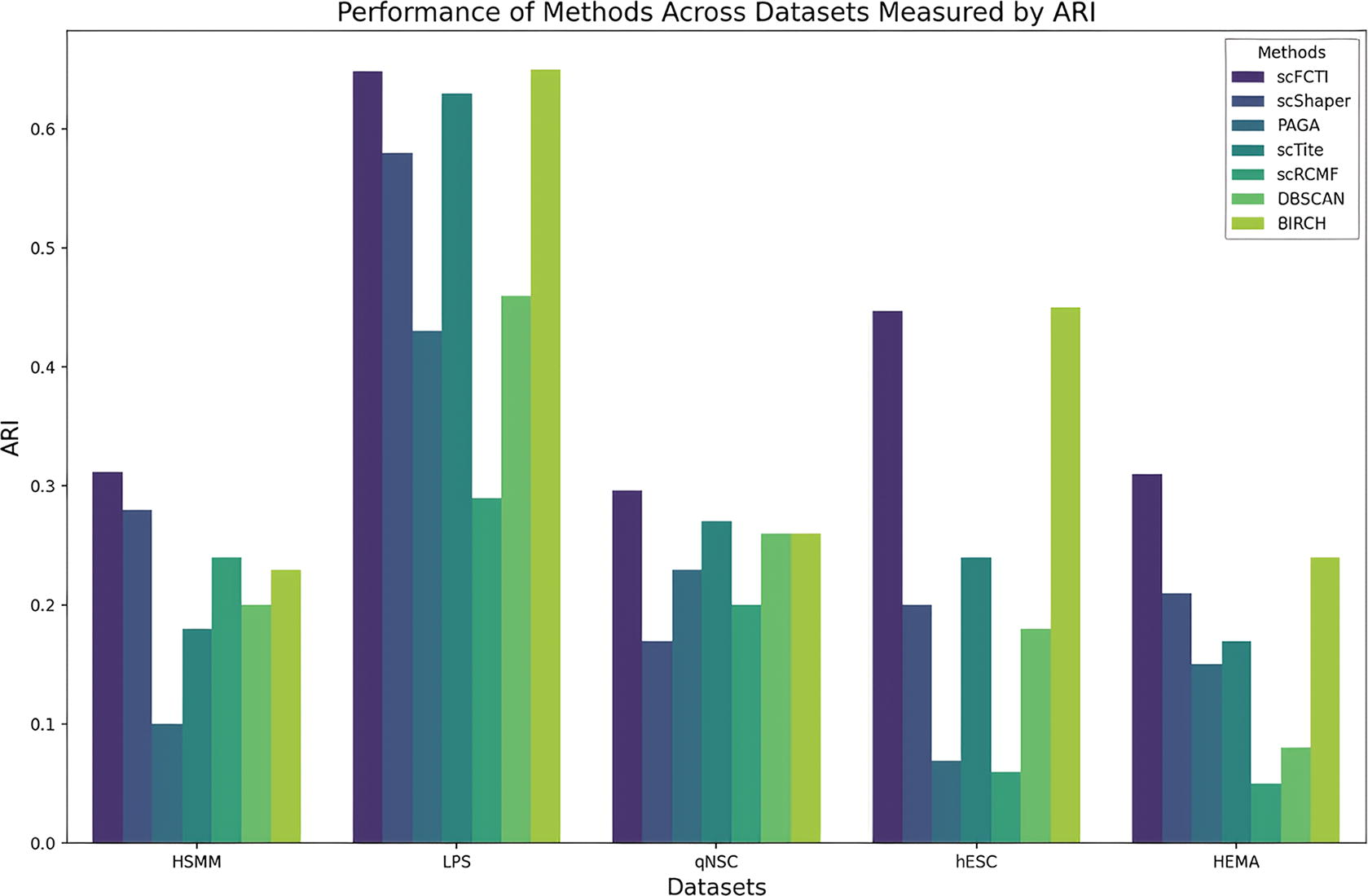
Comparison of different methods. The ARI scores of seven methods are presented in the form of a line graph. Different colors indicate different methods. ARI, Adjusted Rand Index.

FIG. 8.

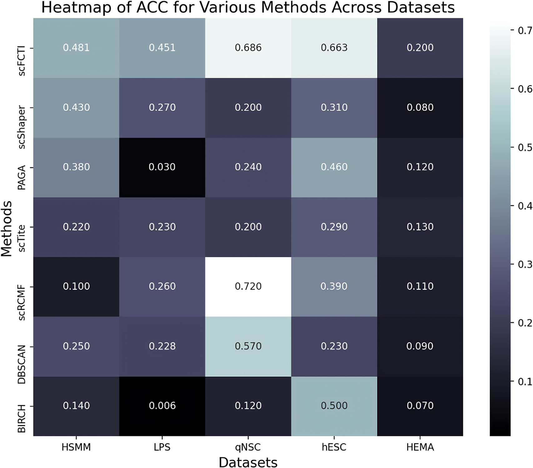
Comparison of different methods. The performance of seven methods in terms of ACC is shown in a heatmap format. The lighter the color, the better the effect. ACC, ACCuracy.

FIG. 9.

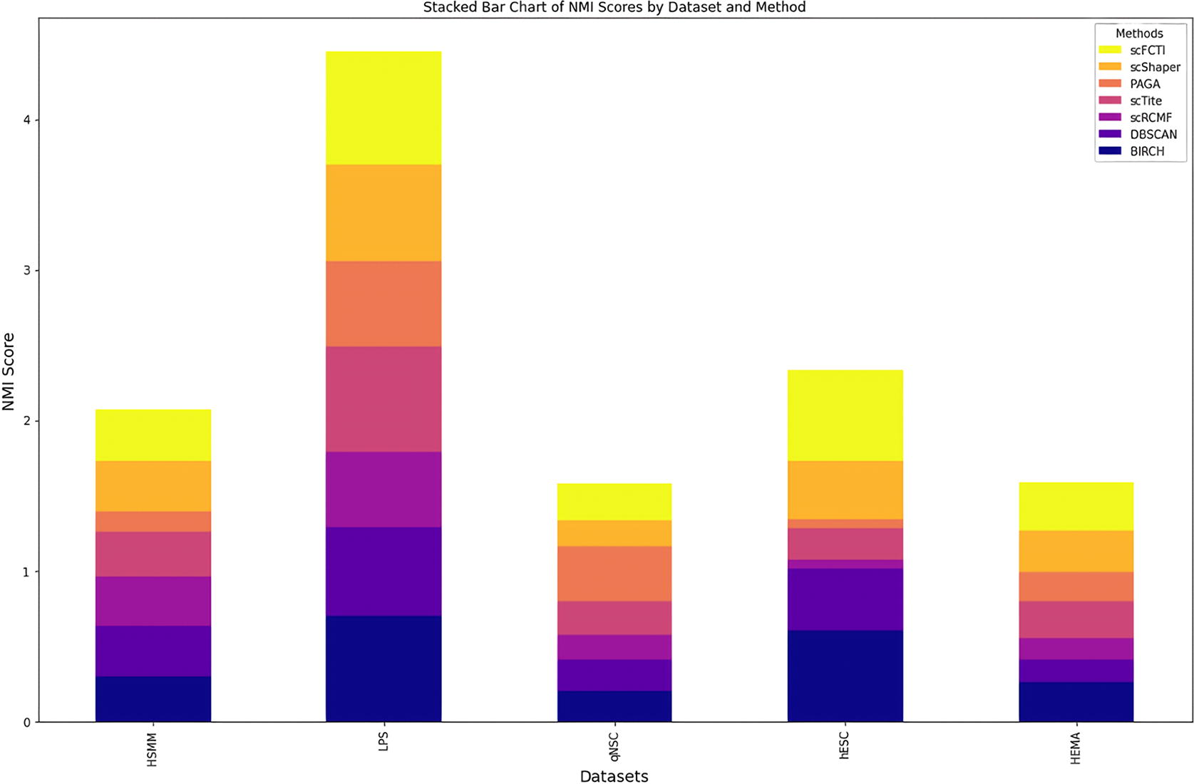
Comparison of different methods. The performance of seven methods in terms of NMI is shown in a stacked bar chart format. The larger the bar area, the better the effect. NMI, Normalized Mutual Information.

To further substantiate the efficacy of scFCTI, we compute the ACC of the seven methods on the five datasets, as illustrated in Figure 8. In order to observe the changes in ACC value more clearly, there is a heat map format of ACC. The lighter the color, the better the effect. The results in the figure unequivocally demonstrate that scFCTI consistently attains the highest score across all datasets. On the hESC dataset, scFCTI achieves an exceptional score of 0.6631, which surpasses the scores of PAGA and scRCMF by 20% and 17%, respectively. In the qNSC dataset, scRCMF achieves the highest score of 0.72, which may be attributed to the suitability of the matrix factorization approach for this dataset.

We also calculate the NMI values for seven methods on five datasets, which are shown in a stacked bar graph (Fig. 9). The higher the NMI, the larger the area on the stacked bar chart. scFCTI do not have a clear advantage in every dataset. Especially compared with the BIRCH method, scFCTI even performs worse than BIRCH on individual datasets. This could be due to the fact that the calculation principle of NMI does not take into account the order of labels, and the results of BIRCH happen have disordered label sequences. At the same time, for some datasets with potential spherical cluster structures, the results of scFCTI are not particularly satisfactory. Generally, combining all the datasets and methods, the performance of scFCTI is the most stable and achieves better results.

scFCTI is a TI method based on soft clustering, which is significantly different from hard clustering represented by Kmeans. Therefore, we also compare scFCTI with Kmeans for different number of starts. Depending on the size of the datasets, the value ranges from 10 to 10,000. ACC is chosen as the evaluation criterion, as shown in Figure 10 and Supplementary Fig. S10. The results of scFCTI are represented on the graph by the red dashed line. Obviously, the result of Kmeans is as sensitive to the choice of the number of starts as expected. Upon comparison, it is determined that employing supervised hard methods such as Kmeans carries risks for further analysis.

FIG. 10.

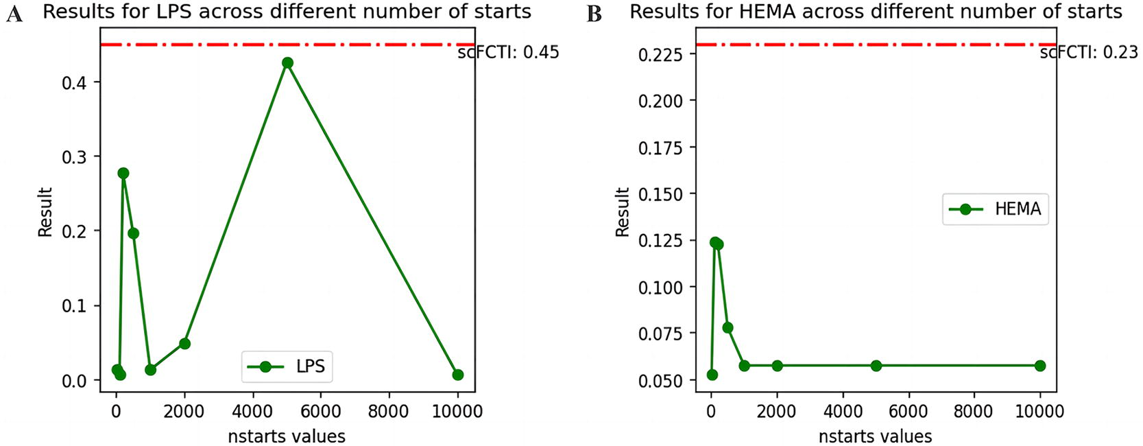
The ACC scores of different numbers of starts in the datasets of LPS and HEMA. The scFCTI’s scores are marked with a red dotted line. (A) The ACC scores in LPS. (B) The ACC scores in HEMA.

As we all know, TI not only reconstructs the trajectory, but also involves the estimation of pseudo-time. In order to analyze the performance of scFCTI from multiple angles, we compare the correlation between pseudo-time and real time on simulated datasets. The simulated datasets in this article contain four structures, linear, bifurcating, cycletree, and multicycles (Fig. 11; Supplementary Fig. S11). The distributions of pseudo-time and real time are described using Kernel Density Estimation. It is evident that although the estimated pseudo-time does not achieve perfect alignment with the actual time, scFCTI successfully captures a similar developmental trend to the original time. This finding further supports the validity and effectiveness of incorporating transitional clusters.

FIG. 11.

Visualization of correlation between pseudo-time and simulation time on different structures of simulation datasets. (A) Visualization of correlation on linear structure. (B) Visualization of correlation on bifurcation structure.

4. CONCLUSION

Some dynamic processes, such as cell differentiation, cell development, and cell fate determination, can be analyzed using gene expression matrices, modeling cell phases and pseudo-times, and ultimately inferring the trajectory of the cell. Probability and membership degrees have emerged as the primary research directions in this field. Notably, TI methods based on probability distribution fit the obtained cluster assignment probabilities to perform subsequent trajectory modeling. However, the number of clusters in a single dataset is often small, which inevitably leads to underfitting when fitting using a probability distribution. Therefore, alternative approaches are needed to address this issue.

To address this issue, we propose a novel method for single-cell TI, called scFCTI. Given a preprocessed gene expression matrix as input, scFCTI uses fuzzy transition clustering and fuzzy transition entropy to partition the cell states more finely, identifying cell populations in stable states and transition states. The latter plays a crucial role in determining subsequent cell branching trajectories and transition paths. Following the basic principle that early-stage cells exhibit high similarity, while mature cells exhibit high heterogeneity (Zhong et al., 2021), scFCTI apply shared nearest-neighbor similarity to determine the starting point of the trajectory. In the end, a cell trajectory with pseudo-time is obtained using the principal curve algorithm.

scFCTI is applied to five real scRNA-seq datasets (HSMM, LPS, qNSC, hESC, and HEMA). Compared to previous experimental results, scFCTI accurately reconstructs the cell trajectories in all datasets. More importantly, compared to the results without transition clusters, scFCTI significantly identifies transition paths and branching trajectories. Based on these transition paths, scFCTI enables more precise reconstruction of the complete cell trajectories. These findings provide further evidence that incorporating membership degree and fuzzy clustering significantly enhances the accuracy of cell classification, thereby providing a robust foundation for subsequent TI.

In summary, this article puts forward scFCTI, a novel TI method based on fuzzy clustering. We demonstrate that scFCTI achieves high precision in reconstructing cell trajectories. scFCTI opens up new possibilities for handling densely connected cell states, and we anticipate that it will become a valuable asset in the study of cellular dynamics. Indeed, scFCTI is not without its limitations. On one hand, since the input for scFCTI is a gene expression matrix, it inherits the common pitfalls of scRNA-seq data, notably the lack of directionality in transcriptional activity. scFCTI employs the sNN algorithm to determine the path direction, but future work could yield different outcomes if integrated with RNA velocity. On the other hand, this paper focuses on studying transition cells representing different states through a specialized clustering. This implies that there is substantial room for advancement in pseudo-time computation, particularly by incorporating the aforementioned RNA velocity.

In downstream analysis, based on TI, multiple sets of learning trajectory can be aligned and analyzed using the inferred results. Trajectory alignment is a popular research area currently. By aligning and analyzing trajectories (Sugihara et al., 2022), key factors can be identified in biological processes, enhancing our understanding of the mechanisms that drive biological systems. Furthermore, taking TI as a starting point, it is meaningful to investigate relevant gene regulatory networks (Kim et al., 2023) from another perspective to unravel crucial information embedded in the trajectories. In recent years, the continuous advancement of multiomics integration technology has made it possible to analyze cellular status by combining multimodal data (Pan and Zhang, 2024). The dynamic processes of cell states are not only reflected in transcriptomic data, but also other omics data such as epigenomics and proteomics (Yamada et al., 2021). Consequently, the integration of multiple omics approaches to identify fuzzy cells and infer cell trajectories is a promising avenue for research with great potential.

Footnotes

AUTHORS’ CONTRIBUTIONS

Conceptualization: X.C. and J.G.; Methodology: X.C.; Validation: Y.M. and Y.S.; Software: X.C. and H.W.; Formal analysis: J.G.; Writing—original draft preparation: X.C.; Writing—review and editing: J.G., Y.M., Y.S., H.W., and B.Z. All authors have read and agreed to the published version of the manuscript.

AVAILABILITY OF DATA AND SOFTWARE

The single-cell mRNA-seq datasets can be downloaded from Gene Expression Omnibus (GEO) repository. The corresponding datasets and GEO accession numbers are as follows: HSMM: GSE52529, LPS: GSE17721, qNSC: GSE71485, hESC: GSE64016, HEMA: GSE59114. The codes for performing analyses in this paper are available at . Computational experiments are conducted using the Jupyter Notebook of python on a laptop with an Intel i5-5350U processor running at 1.80 GHz with 8 GB of RAM. The operating system is Windows 10. The version numbers of the main python packages used are as follows: pandas: 1.5.3, anndata: 0.8.0, scanpy: 1.9.5, datatable: 1.0.0, numpy: 1.23.0, networkx: 2.8.8, seaborn: 1.11.1.

AUTHOR DISCLOSURE STATEMENT

The authors declare that they have no known competing financial interests or personal relationships that could have appeared to influence the work reported in this article.

FUNDING INFORMATION

This work is supported by the National Natural Science Foundation of China (Grant Nos. 12271216 and 11831015).

SUPPLEMENTARY MATERIAL

References

Amit

, Garber

, Chevrier

, et al. Unbiased reconstruction of a mammalian transcriptional network mediating pathogen responses. Science, 2009; 326(5950):257–263; doi: 10.1126/science.1179050

Becht

, McInnes

, Healy

, et al. Dimensionality reduction for visualizing single-cell data using UMAP. Nat Biotechnol, 2018; 37:38–44; doi: 10.1038/nbt.4314

Busse

, Habgood-Coote

, Clare

, et al. Interferon-Induced protein 44 and interferon-induced protein 44-like restrict replication of respiratory syncytial virus. J Virol, 2020; 94(18):e00297-20; doi: 10.1128/JVI.00297-20

Cannoodt

, Saelens

, Deconinck

, et al. Spearheading future omics analyses using dyngen, a multi-modal simulator of single cells. Nat Commun, 2021; 12(1):3942; doi: 10.1038/s41467-021-24152-2

Cannoodt

, Saelens

, Saeys

. Computational methods for trajectory inference from single-cell transcriptomics. Eur J Immunol, 2016; 46(11):2496–2506; doi: 10.1002/eji.201646347

Chen

, Albergante

, Hsu

, et al. Single-Cell trajectories reconstruction, exploration and mapping of omics data with STREAM. Nat Commun, 2019; 10(1):1903; doi: 10.1038/s41467-019-09670-4

Deconinck

, Cannoodt

, Saelens

, et al. Recent advances in trajectory inference from single-cell omics data. Current Opinion in Systems Biology, 2021; 27:100344; doi: 10.1016/j.coisb.2021.05.005

Ding

, Ren

, Zhang

, et al. A novel stromal lncrna signature reprograms fibroblasts to promote the growth of oral squamous cell carcinoma via LncRNA-CAF/Interleukin-33. Carcinogenesis, 2018; 39(3):397–406; doi: 10.1093/carcin/bgy006

Dong

, Hu

, Fan

, et al. Single-Cell RNA-Seq analysis unveils a prevalent epithelial/mesenchymal hybrid state during mouse organogenesis. Genome Biol, 2018; 19(1):31; doi: 10.1186/s13059-018-1416-2

10.

Gan

, Guo

, et al. entropy-based inference of transition states and cellular trajectory for single-cell transcriptomics. Brief Bioinform, 2022a;23(4):bbac225; doi: 10.1093/bib/bbac225

11.

Gan

, Li

, Guo

, et al. TiC2D: Trajectory inference from single-cell RNA-Seq data using consensus clustering. IEEE/ACM Trans Comput Biol Bioinform, 2022b;19(4):2512–2522; doi: 10.1109/TCBB.2021.3061720

12.

Hicks

, Townes

, Teng

, et al. Missing data and technical variability in single-cell rna-sequencing experiments. Biostatistics, 2018; 19(4):562–578; doi: 10.1093/biostatistics/kxx053

13.

Jin

, Liu

, Peng

, et al. Function analysis of mef2c promoter in muscle differentiation. Biotechnol Appl Biochem, 2017; 64(5):647–656; doi: 10.1002/bab.1524

14.

Kharchenko

. The triumphs and limitations of computational methods for scRNA -Seq. Nat Methods, 2021; 18(7):723–732; doi: 10.1038/s41592-021-01171-x

15.

Kim

, Tran

, Kim

, et al. Gene regulatory network reconstruction: Harnessing the power of single-cell Multi-Omic data. NPJ Syst Biol Appl, 2023; 9(1):51; doi: 10.1038/s41540-023-00312-6

16.

Kobak

, Berens

. The art of using T-SNE for single-cell transcriptomics. Nat Commun, 2019; 10(1):5416; doi: 10.1038/s41467-019-13056-x

17.

Kowalczyk

, Tirosh

, Heckl

, et al. Single-Cell RNA-Seq reveals changes in cell cycle and differentiation programs upon aging of hematopoietic stem cells. Genome Res, 2015; 25(12):1860–1872; doi: 10.1101/gr.192237.115

18.

Lan

, Hutvagner

, Zhang

, et al. Density-Based detection of cell transition states to construct disparate and bifurcating trajectories. Nucleic Acids Res, 2022; 50(21):e122; doi: 10.1093/nar/gkac785

19.

Leng

, Chu

L-F

, Barry

, et al. Oscope identifies oscillatory genes in unsynchronized single-cell RNA-Seq experiments. Nat Methods, 2015; 12(10):947–950; doi: 10.1038/nmeth.3549

20.

Luecken

, Theis

. Current best practices in Single-Cell RNA-Seq analysis: A tutorial. Mol Syst Biol, 2019; 15(6):e8746; doi: 10.15252/msb.20188746

21.

Marco

, Karp

, Guo

, et al. Bifurcation Analysis of Single-Cell Gene Expression Data Reveals Epigenetic Landscape. Proc Natl Acad Sci U S A, 2014; 111(52):E5643–E5650; doi: 10.1073/pnas.1408993111

22.

Moon

, van Dijk

, Wang

, et al. Visualizing structure and transitions in high-dimensional biological data. Nat Biotechnol, 2019; 37(12):1482–1492; doi: 10.1038/s41587-019-0336-3

23.

Pan

, Zhang

. Studying temporal dynamics of single cells: Expression, lineage and regulatory networks. Biophys Rev, 2024; 16(1):57–67; doi: 10.1007/s12551-023-01090-5

24.

Pasin

, Gonenc

. An investigation into epidemiological situations of COVID-19 with Fuzzy K-Means and K-Prototype Clustering Methods. Sci Rep, 2023; 13(1):6255; doi: 10.1038/s41598-023-33214-y

25.

Ringnér

. What is principal component analysis? Nat Biotechnol, 2008; 26(3):303–304; doi: 10.1038/nbt0308-303

26.

Ruspini

. Numerical methods for fuzzy clustering. Information Sciences, 1970; 2(3):319–350; doi: 10.1016/S0020-0255(70)80056-1

27.

Saelens

, Cannoodt

, Todorov

, et al. A comparison of single-cell trajectory inference methods. Nat Biotechnol, 2019; 37(5):547–554; doi: 10.1038/s41587-019-0071-9

28.

Shin

, Berg

, Zhu

, et al. Single-Cell RNA-Seq with Waterfall Reveals Molecular Cascades Underlying Adult Neurogenesis. Cell Stem Cell, 2015; 17(3):360–372; doi: 10.1016/j.stem.2015.07.013

29.

Smolander

, Junttila

, Venäläinen

, et al. scShaper: An ensemble method for fast and accurate linear trajectory inference from Single-Cell RNA-Seq Data. Bioinformatics, 2022; 38(5):1328–1335; doi: 10.1093/bioinformatics/btab831

30.

Street

, Risso

, Fletcher

, et al. Slingshot: Cell lineage and pseudotime inference for single-cell transcriptomics. BMC Genomics, 2018; 19(1):477; doi: 10.1186/s12864-018-4772-0

31.

Sugihara

, Kato

, Mori

, et al. Alignment of single-cell trajectory trees with capital. Nat Commun, 2022; 13(1):5972; doi: 10.1038/s41467-022-33681-3

32.

Sun

, Cerabona

, He

, et al. Cdkn3 knockout mice develop hematopoietic malignancies. Blood, 2016; 128(22):1537–1537; doi: 10.1182/blood.V128.22.1537

33.

Trapnell

, Cacchiarelli

, Grimsby

, et al. The dynamics and regulators of cell fate decisions are revealed by pseudotemporal ordering of single cells. Nat Biotechnol, 2014; 32(4):381–386; doi: 10.1038/nbt.2859

34.

van

, Sharma

, Nainys

, et al. Recovering gene interactions from single-cell data using data diffusion. Cell, 2018; 174(3):716–729.e27; doi: 10.1016/j.cell.2018.05.061

35.

Wang

, Zhong

, Ye

, et al. MarkovHC: Markov hierarchical clustering for the topological structure of high-dimensional single-cell omics data with transition pathway and critical point detection. Nucleic Acids Res, 2022; 50(1):46–56; doi: 10.1093/nar/gkab1132

36.

Wolf

, Hamey

, Plass

, et al. PAGA: Graph abstraction reconciles clustering with trajectory inference through a topology preserving map of single cells. Genome Biol, 2019; 20(1):59; doi: 10.1186/s13059-019-1663-x

37.

Yamada

, Okada

, Wang

, et al. Interpretation of omics data analyses. J Hum Genet, 2021; 66(1):93–102; doi: 10.1038/s10038-020-0763-5

38.

Zhang

, Ramakrishnan

, Livny

. BIRCH: A new data clustering algorithm and its applications. Data Mining and Knowledge Discovery, 1997; 1(2):141–182; doi: 10.1023/A1009783824328

39.

Zhang

, Tran

, Nguyen

, et al. A Robust and accurate single-cell data trajectory inference method using ensemble pseudotime. BMC Bioinformatics, 2023; 24(1):55; doi: 10.1186/s12859-023-05179-2

40.

Zhang

, Cui

, Lin

, et al. Critical downstream analysis steps for single-Cell RNA sequencing data. Brief Bioinform, 2021; 22(5):bbab105; doi: 10.1093/bib/bbab105

41.

Zheng

, Wang

, Lin

, et al. IFI44 Is an immune evasion biomarker for sars-cov-2 and staphylococcus aureus infection in patients with RA. Front Immunol, 2022; 13:1013322; doi: 10.3389/fimmu.2022.1013322

42.

Zheng

, Jin

, Nie

, et al. scRCMF: Identification of cell subpopulations and transition states from single-cell transcriptomes. IEEE Trans Biomed Eng, 2020; 67(5):1418–1428; doi: 10.1109/TBME.2019.2937228

43.

Zhong

, Han

, Chen

, et al. SGAE: Single-cell gene association entropy for revealing critical states of cell transitions during embryonic development. Brief Bioinform, 2023; 24(6):bbad366; doi: 10.1093/bib/bbad366

44.

Zhong

, Han

, Wang

, et al. Identifying the critical state of complex biological systems by the directed-network rank score method. Bioinformatics, 2022; 38(24):5398–5405; doi: 10.1093/bioinformatics/btac707

45.

Zhong

, Han

, Zhang

, et al. scGET: Predicting cell fate transition during early embryonic development by single-cell graph entropy. Genomics Proteomics Bioinformatics, 2021; 19(3):461–474; doi: 10.1016/j.gpb.2020.11.008

46.

Zhou

, Zhou

, Cao

, et al. Approaches for scaling DBSCAN algorithm to large spatial databases. J Comput Sci & Technol, 2000; 15(6):509–526; doi: 10.1007/BF02948834

Supplementary Material

Please find the following supplemental material available below.

For Open Access articles published under a Creative Commons License, all supplemental material carries the same license as the article it is associated with.

For non-Open Access articles published, all supplemental material carries a non-exclusive license, and permission requests for re-use of supplemental material or any part of supplemental material shall be sent directly to the copyright owner as specified in the copyright notice associated with the article.

0.00 MB

1.08 MB

0.51 MB

0.57 MB

0.68 MB

0.06 MB

0.10 MB

0.05 MB

0.06 MB

0.05 MB

1.36 MB

0.38 MB

0.28 MB

0.08 MB

1.64 MB

0.45 MB

0.26 MB

0.79 MB