Correcting for Observation Bias in Cancer Progression Modeling

Abstract

Tumor progression is driven by the accumulation of genetic alterations, including both point mutations and copy number changes. Understanding the temporal sequence of these events is crucial for comprehending the disease but is not directly discernible from cross-sectional genomic data. Cancer progression models, including Mutual Hazard Networks (MHNs), aim to reconstruct the dynamics of tumor progression by learning the causal interactions between genetic events based on their co-occurrence patterns in cross-sectional data. Here, we highlight a commonly overlooked bias in cross-sectional datasets that can distort progression modeling. Tumors become clinically detectable when they cause symptoms or are identified through imaging or tests. Detection factors, such as size, inflammation (fever, fatigue), and elevated biochemical markers, are influenced by genomic alterations. Ignoring these effects leads to “conditioning on a collider” bias, where events making the tumor more observable appear anticorrelated, creating false suppressive effects or masking promoting effects among genetic events. We enhance MHNs by incorporating the effects of genetic progression events on the inclusion of a tumor in a dataset, thus correcting for collider bias. We derive an efficient tensor formula for the likelihood function and apply it to two datasets from the MSK-IMPACT study. In colon adenocarcinoma, we observe a significantly higher rate of clinical detection for TP53-positive tumors, while in lung adenocarcinoma, the same is true for EGFR-positive tumors. Compared to classical MHNs, this approach eliminates several spurious suppressive interactions and uncovers multiple promoting effects.

1. INTRODUCTION

Cancer progression models (CPMs) aim to describe and reproduce the evolutionary development of a healthy tissue into a malignant tumor, driven by a series of genetic events such as mutations or copy number alterations (Beerenwinkel et al., 2014). Such events initially occur in single cells through largely random mutagenic processes, but their expansion across the cancer cell population is driven by nonrandom fitness effects they exert in the given environment and the genetic background (Mina et al., 2022). In other words, the fixation of a new event can be promoted or suppressed by previously fixated events, which constrains the probable chronological sequences of events and their co-occurrence patterns (Nowell, 1976).

For example, an initial mutation might promote growth until the tumor is starved for oxygen, whereupon subsequent mutations become beneficial and facilitate blood vessel formation. Access to blood vessels in turn sets the stage for further events culminating in metastasis. Conversely, some events can also suppress one another. This can result, for example, from synthetic lethality, where some events aid the tumor cell individually but become fatal when they occur together. Or, events may target genes in the same regulatory pathway; whichever event occurs first disrupts the whole pathway, reducing selective pressure on the other event.

At large, such interactions between events are still poorly characterized, and learning them from data is the goal of CPMs. The challenge lies in the inherent limitations of available data. Datasets with many patients typically provide only bulk genotypes and do not reliably resolve clonal structures. Most datasets are also cross-sectional. They provide a snapshot of many different tumors at a single time point each but do not track tumors over multiple stages of their evolution.

While we do not know the time at which a tumor was observed relative to the start of its progression, it is also not entirely random. During the initial stages, cancers are low in cell numbers, have accumulated few events, and are generally hard to detect. Instead, most human cancer data comes from advanced stages, after the tumor has clinically progressed and accumulated genetic events. Importantly, some of these genetic events contribute to the cancer’s phenotype: crucial driver genes accelerate proliferation and therefore promote aggressiveness and detectability. Hence, our ability to observe and study tumors depends on the events that occurred before we could detect the tumor. This dependence introduces a systematic bias to CPMs, which we resolve in this article.

So far, CPMs have been developed that can be learned from bulk genotypes (Diaz-Uriarte, 2023) under the assumption that tumors were observed at a random time independent of their progression events. The CPMs are trained on the co-occurrence patterns of events and model the probabilities of future events as functions of the events that are already present. These functions define a causal network. CPMs build on the seminal work of Fearon and Vogelstein (Fearon and Vogelstein, 1990) who manually inferred from genetic and clinical data that colorectal cancer tends to progress along a chain of mutations in the genes APC → KRAS → TP53.

Oncogenetic trees (Beerenwinkel et al., 2005; Desper et al., 1999) extend such chains and allow each event to be a necessary precursor to more than one successor event. In Conjunctive Bayesian Networks (CBNs) (Beerenwinkel et al., 2007; Gerstung et al., 2009; Montazeri et al., 2016), events may also require multiple precursors, thus extending trees to directed acyclic graphs (DAGs). CAPRESE (Loohuis et al., 2014) and CAPRI (Ramazzotti et al., 2015) are similar tree and DAG models where precursor events are not strictly necessary for successor events but raise their probabilities. Other DAG models with different functional forms are Disjunctive Bayesian Networks (Nicol et al., 2021), (Semi-)Monotone Bayesian Networks (Farahani and Lagergren, 2013), and Bayesian Mutation Landscapes (Misra et al., 2014). Pathway Linear Progression Models (Raphael and Vandin, 2015) infer groups of mutually exclusive events and arrange the groups in a chain. PathTiMEx (Cristea et al., 2017) generalizes this to CBNs of groups of mutually exclusive events. Network Aberration Models (NAMs) (Hjelm et al., 2006) are cyclic causal networks with promoting effects. HyperTraPS (Greenbury et al., 2020; Johnston and Williams, 2016) and Mutual Hazard Networks (MHNs) (Schill et al., 2019) generalize this to cyclic networks with promoting and suppressive effects. Similar approaches (Alfaro-Murillo and Townsend, 2023; Moen and Johnston, 2022) allow higher-order rather than pairwise interactions between events. TreeMHN (Luo et al., 2023) infers MHNs from intratumor phylogenetic trees derived from single-cell, multiregion, or bulk sequencing data.

Here we address a fundamental oversight in all these CPMs: They do not include the observation of the tumor itself in their causal networks. Instead, we regard observation of the tumor as an additional event indicating that the tumor was biopsied, sequenced, and eventually included in the dataset. It implies that the tumor has become conspicuous due to its size, morphology, or symptoms such as weight loss, fatigue, or pain. Since a dataset contains by definition only tumors at their moment of observation, neglecting any causal effects on this event makes CPMs prone to the notorious “conditioning on a collider” bias (Hernán MA, 2020). This bias is also known as Berkson’s paradox and refers to spurious associations between any variables that affect another conditioned variable. Joseph Berkson originally described it for a hospital in-patient population, which showed a negative association between diabetes and cholecystitis (Berkson, 1946), see Figure 1. However, since diabetes is known to increase the risk for cholecystitis (Cho et al., 2010), one would naturally expect a positive association. The explanation for the spurious negative association is that diabetes and cholecystitis are both separate causes of being in the hospital and therefore to be observed in this study. Learning of one cause explains away the need for the other cause.

FIG. 1.

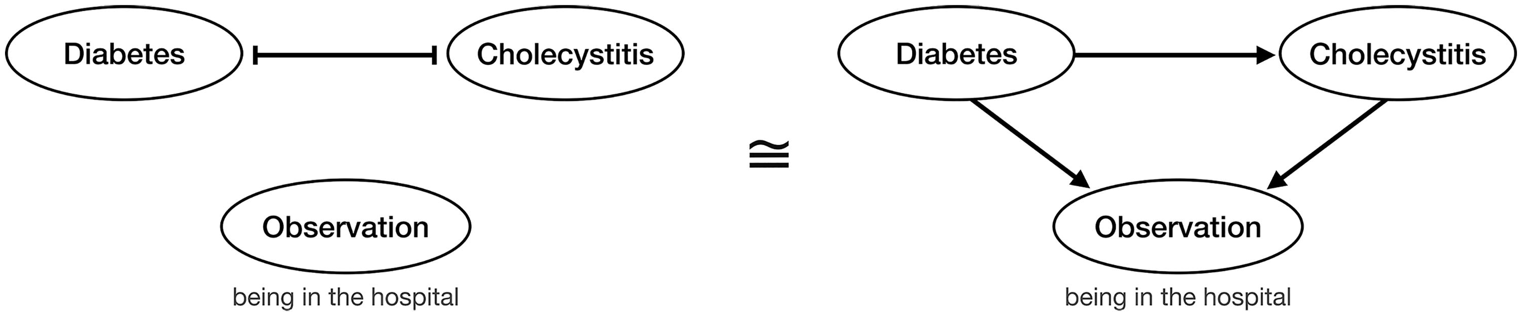
Berkson’s original example of a collider bias (Berkson, 1946): The negative association between diabetes and cholecystitis observed in hospital patients could be spuriously explained (left) by suppressive effects between the diseases if the inclusion of a patient in the dataset were independent of both diseases. Alternatively, the same negative association between diabetes and cholecystitis can be correctly explained (right) by taking into account that both diseases have a promoting effect on being in the hospital and thus observed in the dataset. The spurious association masks the actual promoting effect of diabetes on cholecystitis.

Similarly, the inference of CPMs from statistical associations can be grossly distorted when the observation should be a part of the causal network but is not properly accounted for. CBNs and MHNs are models in continuous time that do have a random observation event, but its rate is fixed at 1 and cannot be affected by other events. Timed Hazard Networks (Chen, 2023) extend MHNs by hidden variables for the observation times of all tumors, but these are also not affected by other events. NAMs (Hjelm et al., 2006) have an observation event whose rate depends on the total number of events that have occurred, but not on which particular events have occurred.

In this article, we extend MHNs by causal effects between their progression events and their observation event. Each event occurs at its base rate and has multiplicative effects on the rate of every other event. These effects can be greater than 1 (promoting), less than 1 (suppressive), or equal to 1 (neutral) and define a causal network with cycles. An MHN is a generative model of cancer progression in the form of a continuous-time Markov chain. We provide an analytical formula for its probability distribution over tumor states, explicitly conditioned on their times of observation. This formula uses tensor expressions which allows us to efficiently infer base rates and multiplicative effects between events via maximum likelihood estimation.

We demonstrate our approach on two datasets of colon adenocarcinoma (COAD) and lung adenocarcinoma (LUAD) from the MSK-IMPACT study (Nguyen et al., 2022; Pugh et al., 2022). Compared to classical MHNs (cMHNs), we find results that offer drastically different interpretations. In COAD, we find that TP53 strongly promotes observation, which explains away suppressive interactions and uncovers promoting effects between APC and TP53. For LUAD, the new model identifies EGFR mutations as principal observation drivers, which explains away its suppressive interactions with most other events but retains suppressive effects with KRAS.

2. METHODS

We first summarize the definition of cMHNs from Schill et al. (2019). Then we extend MHNs by effects on the observation and derive a formula for their likelihood function. Finally, we show that such models are not uniquely identifiable from cross-sectional data and resolve this by a regularization that favors parsimony.

2.1. Classical MHNs with unaffected observation

MHNs (Schill et al., 2019) model cancer progression as a continuous-time Markov chain that describes how a tumor accumulates n possible progression events. Over the course of its progression, a tumor can be in any of $2^{n}$ states $x \in {0, 1}^{n}$ where $x_{i} = 0$ encodes that event $i \in {1, \dots, n}$ has not yet occurred and $x_{i} = 1$ that it has. We assume that every tumor starts at time t = 0 in the healthy state ${(0, \dots, 0)}^{⊤} \in {0, 1}^{n}$ , accumulates events irreversibly one after another, and is finally observed at a random time t which is unknown.

Let $p (t)$ be a vector of size $2^{n}$ that denotes the transient probability distribution over states at time $t \geq 0$ . Here we use a lexicographic order on ${0, 1}^{n}$ with the leftmost bit cycling fastest, see Figure 2 (bottom left). An entry $p {(t)}_{x}$ denotes the probability that a tumor is in state x at time $t \geq 0$ . The initial distribution $p (0) : = {(1, 0, \dots, 0)}^{⊤} \in {[0, 1]}^{2^{n}}$ (1)is concentrated on the healthy state. Its change over time is governed by the Kolmogorov forward equation: $\frac{d p (t)}{d t} = Q p (t) with solution p (t) = \exp (t Q) p (0) .$ (2)

FIG. 2.

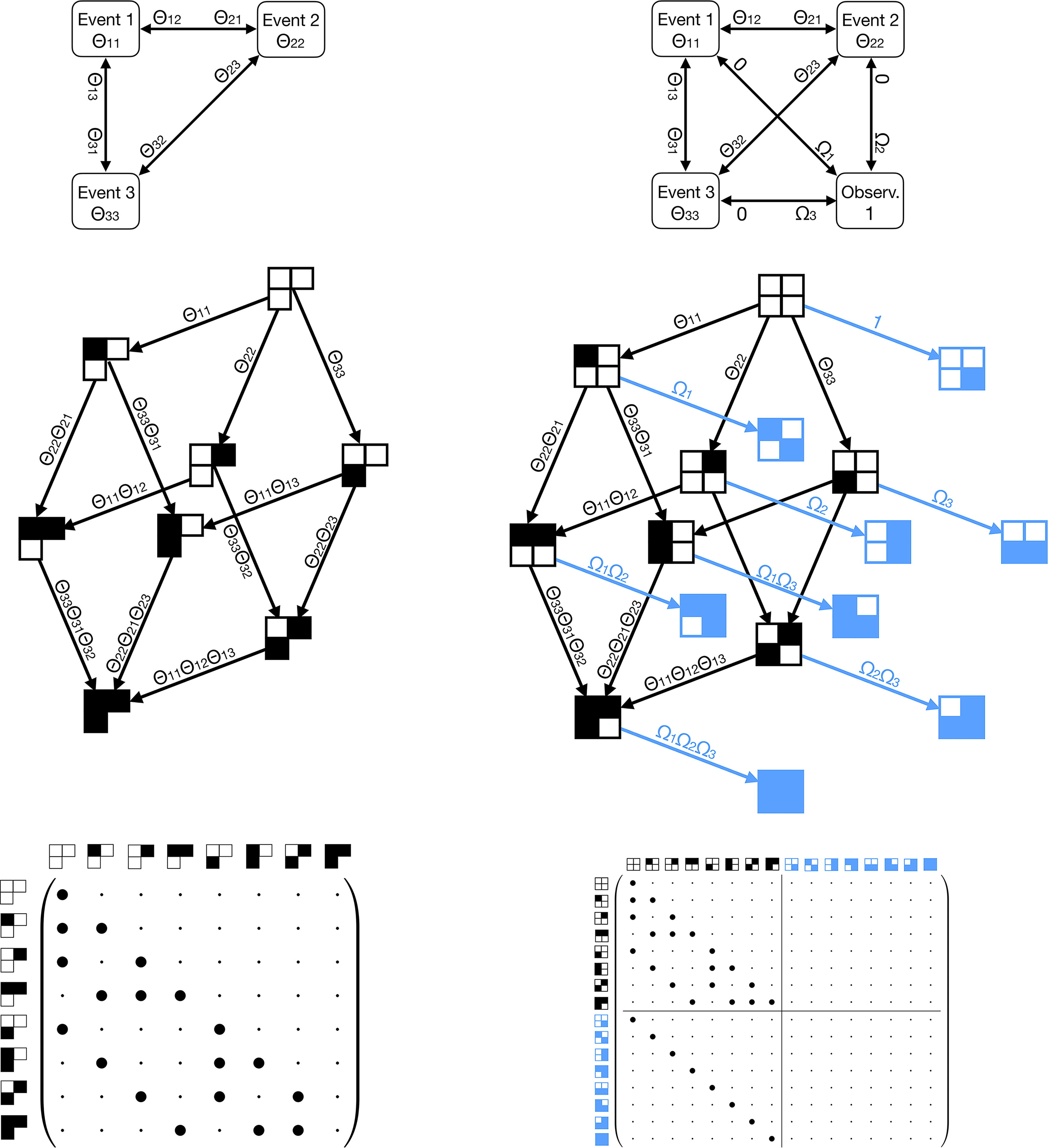
Comparative illustration for n = 3 progression events. Left: A cMHN with parameters Θ and implicit observation event whose rate is fixed at 1. Right: An oMHN with the observation as an explicit fourth event and parameters $(Θ, Ω)$ . Top: the corresponding causal interaction networks between events. Middle: the parameterized transition rates of the corresponding Markov chains. Bottom: the structure of the corresponding transition rate matrices for a lexicographic order of the state space. cMHN, classical Mutual Hazard Network; oMHN, observation MHN.

Here, $Q \in ℝ^{2^{n} \times 2^{n}}$ is the transition rate matrix, where an off-diagonal entry $Q_{x_{+ i}, x}$ is the transition rate from a state $x = {(\dots, x_{i - 1}, 0, x_{i + 1}, \dots)}^{⊤}$ , which lacks event i, to the state $x_{+ i} : = {(\dots, x_{i - 1}, 1, x_{i + 1}, \dots)}^{⊤}$ , which differs from $x$ only in the additional event i. By assumption, events accumulate irreversibly one at a time, and thus all other off-diagonal entries are 0 and Q is lower-triangular. Its diagonal entries are defined such that each column sums to 0. See Figure 2 (bottom left) for an illustration of the structure of Q.

Our aim is to learn for each event i how its rate depends on already present events in $x$ . To this end, an MHN with parameters $Θ \in ℝ^{n \times n}$ defines the functional form $Q_{x_{+ i}, x} = Θ_{i i} \prod_{x_{j} = 1} Θ_{i j},$ (3)where $Θ_{i i} > 0$ is the base rate of event i and $Θ_{i j} > 0$ is the multiplicative effect of event j on the rate of event i. See Figure 2 (middle left) for an illustration of the parameterization of Q.

In order to learn Θ from data via maximum likelihood estimation, we have to compute the probability distribution over all possible tumor states at the time of their observation. The observation in a cMHN occurs randomly at a time which is exponentially distributed with a fixed rate of 1. Marginalizing over the unknown observation time $t \sim Exp (1)$ yields the time-marginal distribution $p : = \int_{0}^{\infty} e^{- t} p (t) d t$ (4) $= \int_{0}^{\infty} \exp (- t I) \exp (t Q) d t = \int_{0}^{\infty} \exp (- t [I - Q]) d t$ (5) $= {[I - Q]}^{- 1} p (0) .$ (6)

Note that equation (5) is only valid for a fixed observation rate, since it relies on the fact that Q commutes with the identity matrix I. The log-likelihood of Θ for a dataset $D$ of observed tumor states is then $ℓ_{D} (Θ) = \frac{1}{| D |} \sum_{x \in D} \log p_{x} .$ (7)

Maximizing the log-likelihood of Θ, for example, via gradient ascent or quasi-Newton methods, requires operations that involve the huge matrix Q. To this end, we make use of the following representation of Q as a sum of tensor products: $Q = \sum_{i = 1}^{n} ⨂_{j = 1}^{i - 1} (\begin{matrix} 1 & 0 \\ 0 & Θ_{i j} \end{matrix}) ⨂ (\begin{matrix} - Θ_{i i} & 0 \\ Θ_{i i} & 0 \end{matrix}) ⨂ ⨂_{j = i + 1}^{n} (\begin{matrix} 1 & 0 \\ 0 & Θ_{i j} \end{matrix}) .$ (8)

Using efficient tensor operations (Buis and Dyksen, 1996), Θ can be learned with a time and storage complexity only exponential in the number of events that have occurred for each tumor, rather than exponential in 2n (Schill, 2022).

2.2. MHNs with Effects on Observation

Here, we extend the cMHN introduced in the previous section to an observation MHN (oMHN). We include the observation event in its causal network as an explicit ${(n + 1)}^{th}$ event. Its base rate is defined as 1 in order to standardize the time scale. We introduce additional parameters $Ω \in ℝ^{n}$ , where $Ω_{j} > 0$ is the multiplicative effect of the progression event $j \in {1, \dots, n}$ on the rate of observation.

Because now the observation rate depends on the state, we can no longer use equation (6) to compute the probabilities of tumor states at their time of observation. Instead, we use the following construction: We set the outgoing effects of the observation on all genetic progression events to 0. Once the observation occurs, it prevents all other events from ever occurring by multiplying their rates with 0, which freezes the data-generating process at the time of observation.1 The probability distribution at observation now equals the stationary distribution at infinity, which can be computed as follows.

Formally, we define the extended Markov chain on the state space ${0, 1}^{n + 1} = \underset{= : A}{\underset{︸}{({0, 1}^{n} \times {0})}} \cup \underset{= : B}{\underset{︸}{({0, 1}^{n} \times {1})}},$ (9)where A includes all states before observation and B all states after observation. The extended transition rate matrix $\bar{Q}$ is of size $2^{n + 1} \times 2^{n + 1}$ and has the following block structure: $\bar{Q} = (\overset{A}{\overset{︷}{_{U}^{T}}} \overset{B}{\overset{︷}{_{0}^{0}}}) {}_{} B}^{} A} with U : = ⨂_{j = 1}^{n} (_{0}^{1}_{Ω_{j}}^{0}) and T : = Q - U,$ (10)where each block is of size $2^{n} \times 2^{n}$ , see Figure 2 (bottom right). The block U contains all transitions that introduce the observation event. It is diagonal with strictly positive eigenvalues and hence invertible. The block T contains all transitions that introduce a progression event, given by Q in equation (8), and U is subtracted from its diagonal so that each column of $\bar{Q}$ sums to 0. T is lower-triangular with strictly negative eigenvalues and hence also invertible.

The transient distribution $\bar{p} (t)$ of the extended Markov chain can also be organized by blocks and is governed by the Kolmogorov forward equation: $\frac{d \bar{p} (t)}{d t} = Q \bar{p} (t) = (_{U}^{T}_{0}^{0}) (_{\bar{p} B (t)}^{\bar{p} A (t)}) = (_{U \bar{p} A (t)}^{T \bar{p} A (t)}),$ (11)where ${\bar{p}}_{A} (t)$ and ${\bar{p}}_{B} (t)$ are each of size $2^{n}$ and denote the transient distribution restricted to A and B, respectively. Given the initial distribution $\bar{p} (0) = {(1, 0, \dots, 0)}^{⊤}$ , that is, ${\bar{p}}_{A} (0) = p (0) and {\bar{p}}_{B} (0) = {(0, \dots, 0)}^{⊤},$ the solution to the Kolmogorov equation reads ${\bar{p}}_{A} (t) = \exp (t T) {\bar{p}}_{A} (0) = \exp (t T) p (0),$ (12) ${\bar{p}}_{B} (t) = {\bar{p}}_{B} (0) + \int_{0}^{t} U {\bar{p}}_{A} (s) d s = \int_{0}^{t} U \exp (s T) {\bar{p}}_{A} (0) d s$ (13) $= U (\int_{0}^{t} \exp (s T) d s) p (0) = - U (I - \exp (t T)) T^{- 1} p (0) .$ (14)

Because all eigenvalues of T are strictly negative, we can calculate the stationary distribution by $\begin{array}{l} {\bar{p}}_{A} (\infty) : = \lim_{t \to \infty} {\bar{p}}_{A} (t) = \lim_{t \to \infty} \underset{\to 0}{\underset{︸}{\exp (t T)}} p (0) = {(0, \dots, 0)}^{⊤}, \\ {\bar{p}}_{B} (\infty) : = \lim_{t \to \infty} {\bar{p}}_{B} (t) = \lim_{t \to \infty} - U (I - \underset{\to 0}{\underset{︸}{\exp (t T)}}) T^{- 1} p (0) \\ = - U T^{- 1} p (0) = U {[U - Q]}^{- 1} p (0) = {[I - Q U^{- 1}]}^{- 1} p (0) . \end{array}$ (15)

We can now supersede the definition of the time-marginal distribution in equation (6) by the more general expression $p : = {\bar{p}}_{B} (\infty) = {[I - Q U^{- 1}]}^{- 1} p (0) .$ (16)

This includes the classical MHN as a special case, where $Ω_{j} = 1$ for all j and thus U = I.

The log-likelihood of a dataset $D$ of observed tumor states is as follows: $ℓ_{D} (Θ, Ω) = \frac{1}{| D |} \sum_{x \in D} p_{x} .$ (17)

In order to compute and maximize it efficiently, we use the tensor expressions for Q and U, which yield $p = {[I - \sum_{i = 1}^{n} ⨂_{j = 1}^{i - 1} (\begin{matrix} 1 & 0 \\ 0 & Θ_{i j} / Ω_{j} \end{matrix}) ⨂ (\begin{matrix} - Θ_{i i} & 0 \\ Θ_{i i} & 0 \end{matrix}) ⨂ ⨂_{j = i + 1}^{n} (\begin{matrix} 1 & 0 \\ 0 & Θ_{i j} / Ω_{j} \end{matrix})]}^{- 1} p (0) .$ (18)

Learning the parameters Θ and Ω then has the same complexity as for a cMHN, that is, it is exponential in the number of events that have occurred for each tumor.

2.3. Nonidentifiability and Regularization

Note that the formula for the time-marginal distribution of an oMHN (18) is the same as for a cMHN (6) where the parameters Θ _ij are replaced by the fractions $Θ_{i j} / Ω_{j}$ . It follows that an oMHN is not uniquely identifiable from cross-sectional data alone. For any oMHN with parameters Θ and Ω, we can construct a likelihood-equivalent cMHN with $Θ_{i j}^{*} = Θ_{i j} / Ω_{j}$ for $i \neq j$ and $Θ_{i i}^{*} = Θ_{i i}$ , see Figure 3. Although both models generate exactly the same observational data, they have very different causal interpretations. That is, they predict different outcomes of hypothetical intervention experiments. This can be done by setting the system to some desired, possibly unnatural state and propagating it forward in time.

In order to decide on a particular causal model, we cannot rely on data alone but have to incorporate background knowledge or preferences in the form of a Bayesian prior or a penalty on the likelihood. Following the principle of parsimony (Occam’s razor), we prefer simple models that postulate the least number of causal mechanisms for explaining the data. This means that MHNs should be sparse, in the sense that many effects $Θ_{i j} = 1$ and $Ω_{j} = 1$ for $i \neq j$ . In the example of Figure 3, we would hence prefer the model on the right.

FIG. 3.

Example of a cMHN (left) and an oMHN (right), which generate the same observational data but differ in their causal interpretation. They imply different experimental predictions: A drug treatment that suppresses event 2 would increase the probabilities of events 1 and 3 according to the left model, but not according to the right model. (Both networks are fully connected, but neutral effects of multiplicative strength 1 are not drawn.).

Moreover, we prefer symmetric models where many effects $Θ_{i j} = Θ_{j i}$ since these are likely due to a single causal mechanism that is inherently symmetric, such as synthetic lethality or functional equivalence among mutations. While such effects presumably do not vary in strength whether event i or j occurs first, there may be important exceptions (Iranzo et al., 2022; Ortmann et al., 2015).

To this end, we propose maximizing the log-likelihood regularized by the following penalty, which induces sparsity and soft symmetry: $ℓ_{D} (Θ, Ω) - λ (\sum_{i < j} \sqrt{θ_{i j}^{2} + θ_{j i}^{2} - θ_{i j} θ_{j i}} + \sum_{j = 1}^{n} \sqrt{ω_{j}^{2}}),$ (19)where $θ_{i j} : = \log (Θ_{i j}), ω_{j} : = \log (Ω_{j})$ and $λ > 0$ is the hyperparameter. Figure 4 illustrates this penalty in comparison with other common penalties: The standard L1 penalty encourages sparsity such that many logarithmic effects are 0 (hence multiplicative effects are 1). When two counter-directed effects θ_ij and θ_ji cannot be discerned from data, the L1 penalty would prefer a single effect in an arbitrary direction, depending on the initialization. The group L1 penalty (Yuan and Lin, 2005) encourages sparsity between different counter-directed effect pairs, but not within each pair. It therefore allows for symmetric effects but does not encourage them. Our proposed symmetrizing group L1 penalty encourages counter-directed effects to have the same strength and same sign through the additional term $- θ_{i j} θ_{j i}$ .

FIG. 4.

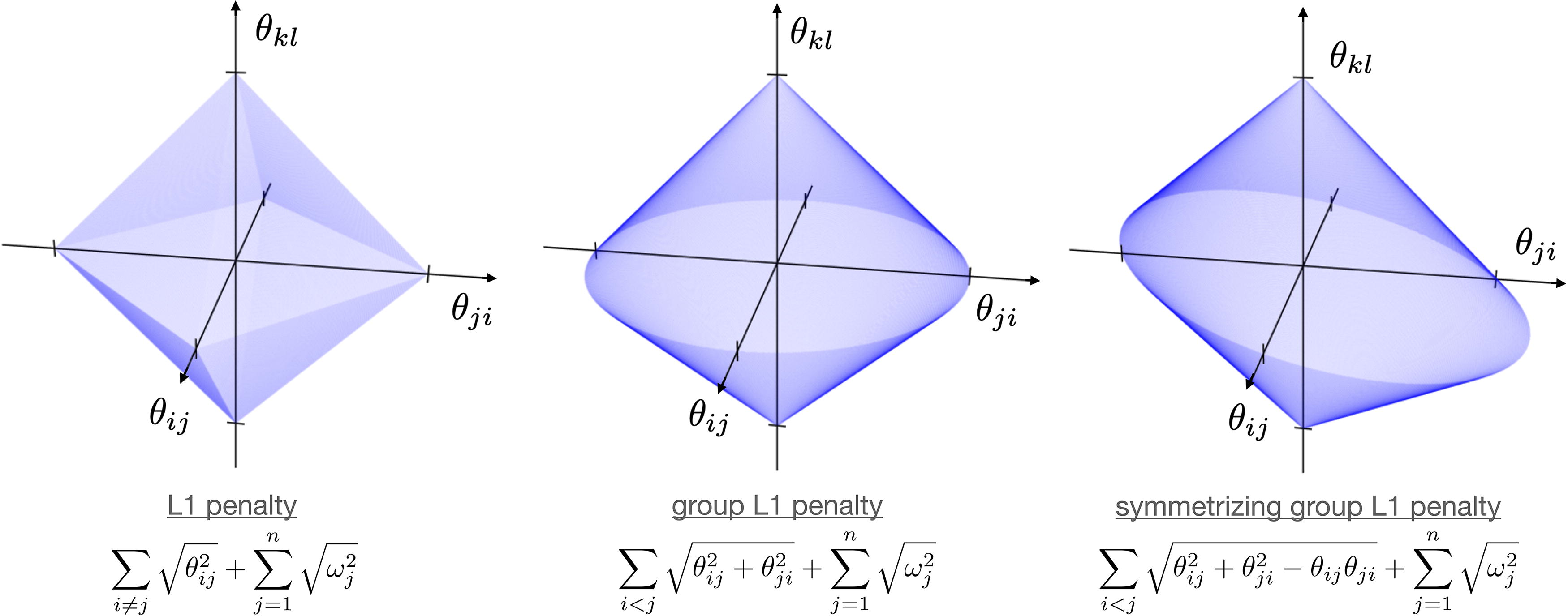
Three possible regularization penalties, visualized by their unit-level surfaces. The horizontal plane corresponds to two counter-directed effects θ_ij and θ_ji, whereas the vertical axis corresponds to an unrelated effect θ_kl. The unit-level curve in the horizontal plane is a square for the L1 penalty, a circle for the group L1 penalty, and an ellipse for the symmetrizing group L1 penalty. The major axis of the ellipse is oriented through the quadrants with equal sign.

This means that, when our algorithm does infer asymmetrical effects despite this penalty, the choice is likely driven by the data. On the other hand, effects that are inferred as symmetric may either be genuinely so, or the direction may not be discerned from the data.

In this article, we choose the hyperparameter λ in 5-fold cross-validation according to the One Standard Error Rule (Hastie et al., 2009), which selects the largest value for λ such that its average log-likelihood is within one standard error of the optimum. We use this rule because the optimal λ tends to 0 for larger datasets as it becomes less necessary to prevent overfitting, but we still want to favor simple models to mitigate nonidentifiability.

3. RESULTS

We provide a new version of MHNs with a corresponding efficient learning algorithm. These models provide a novel perspective on cancer progression by inferring which (genetic) events promote the clinical detection of a tumor. The models are thereby corrected for a collider bias and offer more realistic interpretations of cancer progression, showing fewer spurious interactions and more genuine interactions that had been previously obscured.

We applied our method to cancer genomic data from clinical targeted sequencing assays originally collected by the Memorial Sloan Kettering Cancer Center (Nguyen et al., 2022) and retrieved through AACR GENIE (The AACR Project GENIE Consortium et al., 2017). Specifically, we selected cohorts of primary COAD (n = 2269) and primary LUAD (n = 3662). For each cohort, we selected the 12 most frequently mutated genes as model events while discounting putative nonpathogenic variants and genes that had not been consistently sequenced across assay versions—for more details, see Appendix A1.

Although oMHN models are more realistic than cMHNs, they are in principle equally powerful for explaining the data, so we did not necessarily expect results with higher likelihood. Nevertheless, we validated their model fit by splitting each dataset in half into a training and test set. We trained a cMHN and an oMHN on the training set and evaluated their log-likelihoods on the test set. For COAD, the cMHN achieved a log-likelihood of –5.14, while the oMHN achieved a slightly better –5.10. For reference, the independence model2 achieved –6.02, and the best possible performance was the negative entropy –4.48 of the test set. For LUAD, the cMHN achieved a log-likelihood of –3.96 and the oMHN achieved a slightly better –3.94. The independence model achieved –4.50, and the negative entropy of the test set was –3.74.

In the following, we report the models trained on the full datasets.

3.1. Colon Adenocarcinoma

Mutations in APC, KRAS, and TP53 are classically regarded as the principal genetic drivers of conventional COAD progression (Fearon and Vogelstein, 1990; Vogelstein et al., 2013). The three events are abundant in the dataset (42%−72%) but enriched in samples with few events overall, see Appendix A2. TP53 in particular is anticorrelated with most other events, that is, it is often observed with no or very few co-events.

Although cMHN and oMHN both fit the data similarly well, they offer drastically different causal interpretations (Fig. 5): cMHN suggests that APC, KRAS, and TP53 strongly suppress each other’s accumulation as well as other events. oMHN instead proposes that APC, KRAS, and especially TP53 lead to observation. This explains away many of their suppressive interactions and even uncovers a synergy between APC and TP53.

FIG. 5.

Heatmap visualization of the cMHN (left) and the oMHN (right) for the COAD dataset. In the main heatmap bodies, each cell shows the multiplicative effect Θ _ij from the column event j on the row event i. Promoting effects >1 are coded in red, suppressive effects <1 in blue, and neutral effects = 1 are blank. The additional top row indicates base rates Θ _ii , and the bottom row indicates effects Ω _j from each column event j on the observation event. Values are rounded to the first decimal.

The different causal models also imply different chronological orders of events. We demonstrate this by considering the probabilities of every possible chronological order to reach the state in which APC, KRAS, and TP53 are mutated in Table 1. Contrary to cMHN, the oMHN suggests that APC tends to occur early in the progression and that TP53 tends to occur late, despite its prevalence. This is because TP53 triggers and therefore immediately precedes the observation. In a similar fashion, we analyzed the probabilities of chronological orders for all common genotypes in the data at hand and present in Figure 6 the most probable histories.

FIG. 6.

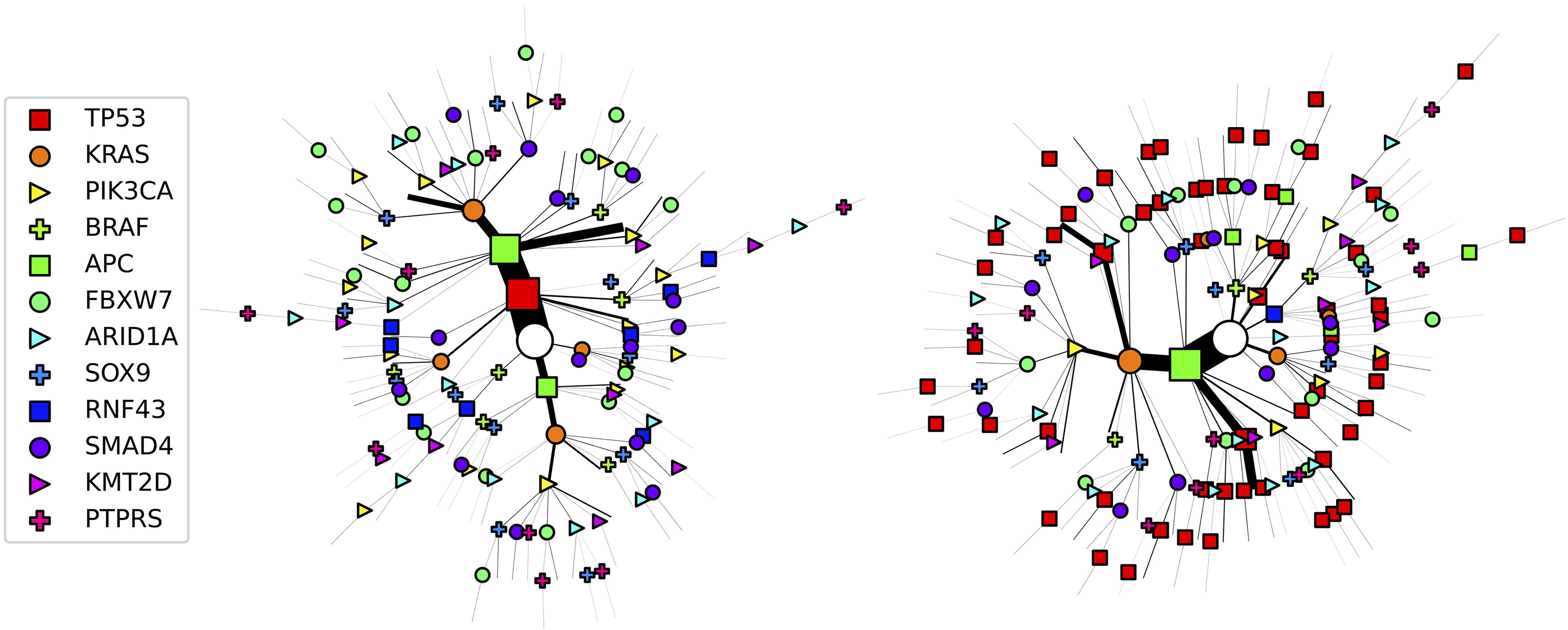
Most probable chronological order of events for the COAD dataset according to the cMHN (left) and oMHN (right). Each path from the root of the tree (white circle) to a leaf represents the progression of a tumor in the dataset. The symbols along the path indicate events whose most probable chronological order was computed from the trained models. To avoid clutter, the observation event at every leaf is implied without drawing a symbol and only tumors whose state is shared by at least three patients are drawn. The size of the edges and symbols along a path scale in the total number of patients with that tumor state. COAD, colon adenocarcinoma.

Table 1.

All Possible Chronological Orders to Reach the Genotype that Contains Exactly the Events APC, KRAS, TP53, and was Observed

Chronological order			cMHN	oMHN
APC	→ KRAS	→ TP53	0.068	0.312
KRAS	→ APC	→ TP53	0.064	0.262
APC	→ TP53	→ KRAS	0.198	0.149
KRAS	→ TP53	→ APC	0.075	0.113
TP53	→ APC	→ KRAS	0.383	0.101
TP53	→ KRAS	→ APC	0.212	0.064

The probabilities of these orders according to cMHN and oMHN are computed as in Appendix A3 and rounded to the third decimal.

Unlike for cMHN, the interpretations drawn from oMHN are in line with common conceptions about COAD genetic progression. Specifically, the model recapitulates the well-researched adenoma-to-carcinoma sequence, which posits that APC inactivation serves as an initial event generating a benign lesion. Only then can auxiliary drivers like TP53 elicit aggressive and invasive growth, which makes the cancer clinically conspicuous (Bürtin et al., 2020; Vogelstein et al., 2013; Yang et al., 2019).

While the biological causes for this interplay continue to be debated, there is ample observational support. In mouse models of colon cancer, APC loss is sufficient to generate benign adenomas, but these are typically spatially confined and noninvasive (Fischer et al., 2013; Johnson and Fleet, 2012). Similarly, in human clinical data, APC inactivation is largely the only driver mutation that is frequently present even in the most microscopic adenomas. Contrary to other driver alterations, its frequency is not substantially higher in more advanced lesions (Fearon, 2011). These insights suggest that APC inactivation is an initiating event in colon tumorigenesis, which is on its own rarely sufficient to generate a clinically conspicuous cancer.

On the other hand, it is known that “secondary” driver mutations, specifically KRAS activation or TP53 inactivation greatly increase tumor growth, aggressiveness, and invasive abilities in mouse models with an APC background (Hadac et al., 2015; Halberg et al., 2000; Sansom et al., 2006). However, experiments suggest that these secondary driver mutations are typically unable to generate viable colon cancers on their own (Harvey et al., 1993; Johnson and Fleet, 2012; Sansom et al., 2006).

The synergy between APC and TP53 is further supported by a systematic study of conditional selection effects in cancer genomes (Iranzo et al., 2022), which found that TP53 mutations are under particularly strong positive selection in APC-mutated colorectal cancers, and vice versa.

Taken together, we report that when correcting for the observation bias, oMHN recapitulates and quantifies established dynamics of colon cancer progression in which APC inactivation initiates rather inconspicuous lesions before synergistic codrivers cause clinical observation.

While introduction of the observation event produced markedly different results, some interactions remain consistent between cMHN and oMHN. Most notably, both models suggest a “double antagonism” between the KRAS-APC and BRAF-RNF43 pairs: each event in one pair suppresses both members of the other pair. In fact, the two event pairs likely produce similar consequences through alternative means: both event pairs deregulate the RAS and Wnt pathways. These are synergistic milestones in COAD progression (Jeong et al., 2018; Lee et al., 2018). Specifically, KRAS and BRAF mutations are alternative ways of RAS pathway deregulation (Cicenas et al., 2017; Oliveira et al., 2006), and APC and RNF43 are alternative ways of Wnt signaling deregulation (Giannakis et al., 2014; Grant et al., 2021). Additionally, the synergy within the pairs as well as the antagonism between them are clearly reflected in the conditional selection analysis of (Iranzo et al., 2022). Both points, functional similarity and conditional selection effects, support genuine antagonism between these pairs.

Interestingly, the BRAF-RNF43 pair is associated with a distinct mode of COAD progression, the Serrated Neoplasia Pathway. These cancers develop from serrated sessile lesions, with different histopathological and prognostic properties (Leggett and Whitehall, 2010). Unlike in conventional COADs, APC mutations are rare here while BRAF mutations are thought to be initial (Bettington et al., 2015; Bond et al., 2016). Experimental evidence suggests that specifically MLH1-deficient, microsatellite-instable serrated COADs rely on BRAF and RNF43 mutations in their progression (Bleijenberg et al., 2022; Yamamoto et al., 2022).

Taken together, these findings suggest that there are two prototypical ways of genetic progression in COAD. On the one hand, any combination of the synergistic triplet APC-KRAS-TP53 can be sufficient to elicit observation, although APC tends to be the initiating factor and TP53 the observation driver. On the other hand, crucial pathway deregulation can also be achieved by alternatives like BRAF and RNF43. In these cases, there is no main observation driver, and typically more alterations are accumulated before observation.

3.2. Lung Adenocarcinoma

In the models on LUAD, Figure 7, we also observed a shift from widespread suppressive interactions in cMHN to observation rate increases in oMHN, most notably for EGFR mutations. EGFR mutations appear mutually exclusive with many other events in the input data. cMHN models this with widespread suppressive interactions, while oMHN explains these away by an observation rate increase. For EGFR and TP53, oMHN even suggests synergy instead of the antagonism proposed by cMHN.

FIG. 7.

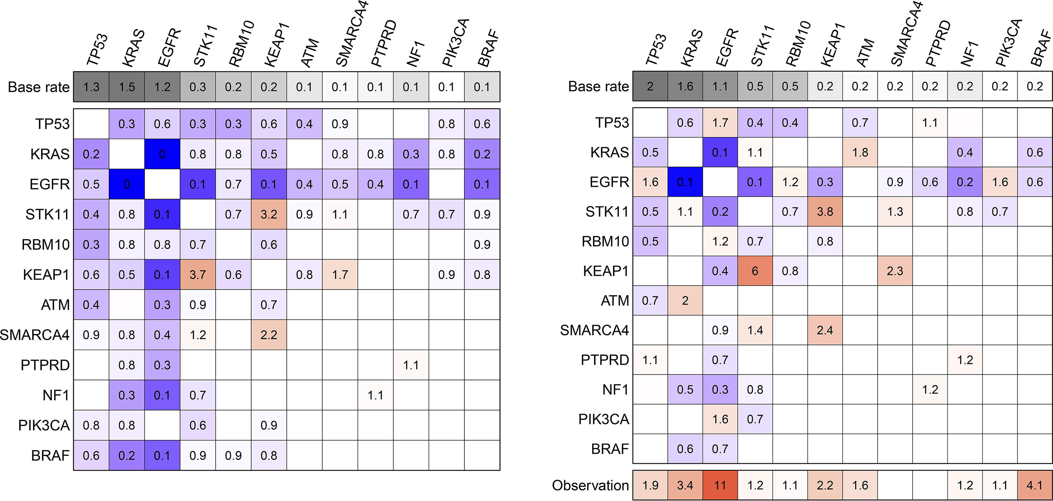
Heatmap visualization of the cMHN (left) and the oMHN (right) for the LUAD dataset. In the main heatmap bodies, each cell shows the multiplicative effect Θ _ij from the column event j on the row event i. Promoting effects >1 are coded in red, suppressive effects <1 in blue, and neutral effects = 1 are blank. The additional top row indicates base rates Θ _ii , and the bottom row indicates effects Ω _j from each column event j on the observation event. Values are rounded to the first decimal. LUAD, lung adenocarcinoma.

The chronological orders differ between cMHN and oMHN mainly for EGFR and KRAS. These events tend to occur later according to oMHN because they trigger observation, see Figure 8. According to oMHN, EGFR has a strong effect on observation on its own. Conversely, KRAS-positive LUADs elicit observation in a more concerted manner supported by, for example, ATM, STK11, and KEAP1. This is in line with in-depth genomic analyses that suggest that EGFR-driven lung cancers are largely self-sufficient, that is, they depend less on concurrent driver mutations, with TP53 co-mutations being a notable exception (Nahar et al., 2018). Moreover, there are also interactions that remain consistent between cMHN and oMHN, most prominently the suppressive relationship between EGFR and KRAS. In fact, experimental demonstration of synthetic lethality (Unni et al., 2015) and conditional selection analysis (Iranzo et al., 2022) both support a genuine antagonism. We also note the synergism between mutations in STK11 and KEAP1, which is consistent between both models (albeit reinforced by oMHN) and possibly reflects their dual role in ferroptosis protection (Wohlhieter et al., 2020).

FIG. 8.

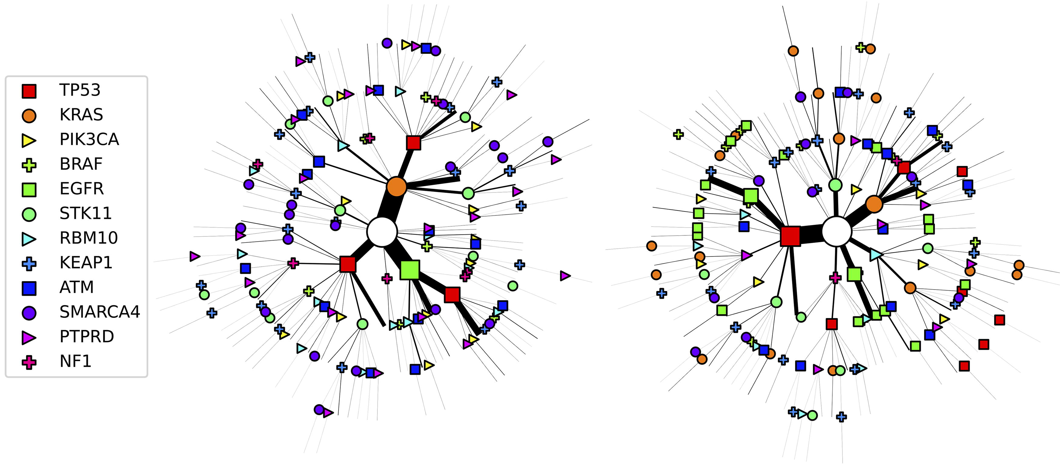
Most probable chronological orders of events for the LUAD dataset according to the cMHN (left) and oMHN (right). Each path from the root of the tree (white circle) to a leaf represents the progression of a tumor in the dataset. The symbols along the path indicate events whose most probable chronological order was computed from the trained models. To avoid clutter, the observation event at every leaf is implied without drawing a symbol, and only tumors whose state is shared by at least three patients are drawn. The size of the edges and symbols along a path scale in the total number of patients with that tumor state.

3.3. Evaluation on Synthetic Data

We evaluated the accuracy of our learning algorithm in simulation experiments. To this end, we used the oMHN inferred from the COAD dataset in Section 3.1 and declared it as the ground truth model. From this model, we simulated 100 synthetic datasets of the same size as the original dataset, that is, 2269 tumors each. For each synthetic dataset, we trained a new oMHN by the same procedure as described before.

The resulting 100 models can be found in the github repository. Figure 9 shows the marginal distributions of each logarithmic entry θ_ij over the 100 simulations. While the estimators show a slight tendency to underestimate the actual strength of the effect, we found that our method accurately recovered whether an effect exists and whether it is promoting or suppressive.

FIG. 9.

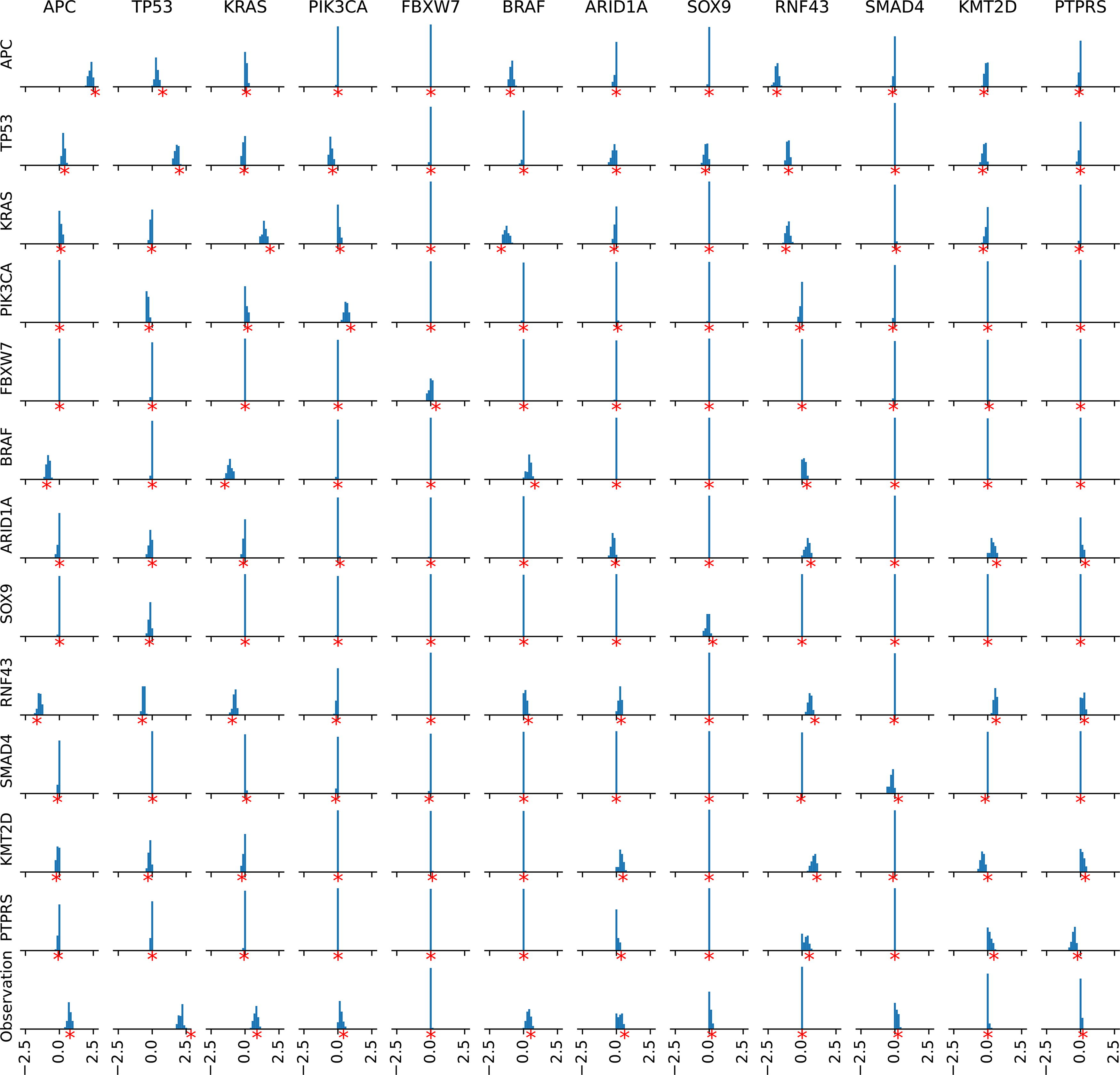
Evaluation of learning accuracy on 100 simulated datasets from a given ground truth model. Each histogram shows the distribution of an entry $θ_{i j} = \log (Θ_{i j})$ over the 100 learned models. The corresponding entry in the ground truth model is indicated by a red star.

4. DISCUSSION

Large cancer genomics datasets offer a valuable opportunity for modeling cancer progression, but many of them are observational, drawn from routine clinical practice rather than controlled trials (The AACR Project GENIE Consortium et al., 2017). This makes them prone to pervasive biases (van de Haar et al., 2019), such as the notorious confounder bias, which is due to unaccounted effects from latent variables, and the collider bias, which is due to unaccounted effects on a conditioned outcome. In this article, we have resolved an important instance of the collider bias by learning which genetic events cause the clinical observation of a tumor.

This is an important biological insight on its own, since the observation of a tumor is often tied to its size and aggressiveness. Here, we find that in COAD, observation is caused by mutations in TP53, consistent with its role as late-stage driver promoting the transition from adenomas to more aggressive carcinomas (Vogelstein et al., 2013; Yang et al., 2019). In contrast, for LUAD, observation is mainly promoted by different driver mutations activating the RTK-RAS pathway, specifically affecting EGFR, BRAF, and KRAS (Imperial et al., 2019). In addition, and perhaps more consequentially, learning such observation effects explains away spurious interactions between many other events and uncovers interactions that were previously hidden, for instance, the synergism between EGFR and TP53 mutations in lung cancer. Overall, the effects inferred by oMHN are more in line with the current literature than the effects inferred by MHN. Despite this, further validation studies, especially of the effects on the observation, are necessary. However, these would require access to data generated by prospective cohort studies.

While resolving the collider bias is a crucial step toward more reliable CPMs, other sources of confounding may still remain. Environmental exposures such as smoking, complex mutational processes, or even the tumor’s cell type of origin can significantly impact the evolution of tumors. Future work should therefore combine our approach with the modeling of these factors, either as latent variables if they are not easily measurable or as additional covariates if they can be measured directly. The observation mechanism introduces an additional source of nonidentifiability to the MHN framework. The exact extent of it is currently not fully resolved and warrants additional comprehensive investigation in future studies. Further nonidentifiability could be mitigated by exploiting known time intervals between consecutive observations (Rupp et al., 2021), such as biopsies of primary tumors and metastases. Surprisingly, Gotovos et al. (2021) have shown that classical MHNs become more identifiable by simply including more events. This, however, necessitates efficient learning algorithms such as (Georg, 2022; Gotovos et al., 2021; Klever et al., 2022). oMHN models the evolution of bulk tumor profiles and thus does not account for intratumor heterogeneity. Nevertheless, our approach could also be used to directly extend models of subclonal tumor progression (Luo et al., 2023).

More realistic models will ultimately allow us to not only understand and predict the course of cancer progression but also inform clinicians about potential outcomes of specific treatment choices and thus impact patient care directly.

5. DATA AND CODE AVAILABILITY

We provide a github repository at https://github.com/cbg-ethz/ObservationMHN to reproduce the results in this article. It also contains the input data that the models were trained on, alongside scripts detailing their preprocessing. The original raw data are part of the GENIE 13.1 data release and obtainable at The AACR Project GENIE Consortium (2023).

Footnotes

ACKNOWLEDGMENTS

The authors thank Tilo Wettig, Simon Pfahler, and Stefan Hansch for their helpful discussions.

AUTHORS’ CONTRIBUTIONS

Conceptualization: R.S., M.K., and K.R. Methodology: R.S., M.K.,Y.L.H., and S.V. Software: S.V. and Y.L.H. Validation: A.L. and Y.L.H. Investigation: A.L. and Y.L.H. Data curation: A.L. Writing—original draft: R.S., M.K., A.L., and Y.L.H. Writing—reviewing and editing: N.B., R.S., and K.R. Visualization: R.S. and Y.L.H. Supervision: N.B., R.S., and L.G.

AUTHOR DISCLOSURE STATEMENT

The authors declare they have no conflicts of interest.

FUNDING INFORMATION

This work was supported by the Swiss National Science Foundation grant 179518, the Swiss Cancer League grant KFS-2977-08-2012, and the German Research Foundation grants TRR-305 and GR-3179/6-1.

Appendix

References

Adzhubei

, Schmidt

, Peshkin

, et al. A method and server for predicting damaging missense mutations. Nat Methods, 2010; 7(4):248–249; doi: 10.1038/nmeth0410-248

Alfaro-Murillo

, Townsend

. Pairwise and higher-order epistatic effects among somatic cancer mutations across oncogenesis. Math Biosci, 2023; 366:109091; doi: 10.1101/2022.01.20.477132

Beerenwinkel

, Eriksson

, Sturmfels

. Conjunctive Bayesian networks. Bernoulli, 2007; 13(4):893–909; doi: 10.3150/07-BEJ6133

Beerenwinkel

, Rahnenführer

, Däumer

, et al. Learning multiple evolutionary pathways from cross-sectional data. J Comput Biol, 2005; 12(6):584–598; doi: 10.1089/cmb.2005.12.584

Beerenwinkel

, Schwarz

, Gerstung

, et al. Cancer evolution: Mathematical models and computational inference. Syst Biol, 2014; 64(1):e1–e25; doi: 10.1093/sysbio/syu081

Berkson

. Limitations of the application of fourfold table analysis to hospital data. Biometrics Bulletin, 1946; 2(3):47–53; doi: 10.2307/3002000

Bettington

, Walker

, Rosty

, et al. Clinicopathological and molecular features of sessile serrated adenomas with dysplasia or carcinoma. Gut, 2015; 66(1):97–106; doi: 10.1136/gutjnl-2015-310456

Bleijenberg

, IJspeert

, Mulder

, et al. The earliest events in BRAF-mutant colorectal cancer: Exome sequencing of sessile serrated lesions with a tiny focus dysplasia or cancer reveals recurring mutations in two distinct progression pathways. J Pathol, 2022; 257(2):239–249; doi: 10.1002/path.5881

Bond

, McKeone

, Kalimutho

, et al. RNF43 and ZNRF3 are commonly altered in serrated pathway colorectal tumorigenesis. Oncotarget, 2016; 7(43):70589–70600; doi: 10.18632/oncotarget.12130

10.

Buis

, Dyksen

. Efficient vector and parallel manipulation of tensor products. ACM Trans Math Softw, 1996; 22(1):18–23; doi: 10.1145/225545.225548

11.

Bürtin

, Mullins

, Linnebacher

. Mouse models of colorectal cancer: Past, present and future perspectives. World J Gastroenterol, 2020; 26(13):1394–1426; doi: 10.3748/wjg.v26.i13.1394

12.

Chakravarty

, Gao

, Phillips

, et al. OncoKB: A precision oncology knowledge base. JCO Precis Oncol, 2017; 2017(1):1–16; doi: 10.1200/po.17.00011

13.

Chen

. Timed hazard networks: Incorporating temporal difference for oncogenetic analysis. PLoS One, 2023; 18(3):e0283004; doi: 10.1371/journal.pone.0283004

14.

Cheng

, Mitchell

, Zehir

, et al. Memorial sloan kettering-integrated mutation profiling of actionable cancer targets (MSK-IMPACT). J Mol Diagnostics, 2015; 17(3):251–264; doi: 10.1016/j.jmoldx.2014.12.006

15.

Cho

, Han

H-S

, Yoon

Y-S

, et al. Risk factors for acute cholecystitis and a complicated clinical course in patients with symptomatic cholelithiasis. Arch Surg, 2010; 145(4):329–333; discussion 333; doi: 10.1001/archsurg.2010.35

16.

Cicenas

, Tamosaitis

, Kvederaviciute

, et al. KRAS, NRAS and BRAF mutations in colorectal cancer and melanoma. Med Oncol, 2017; 34(2):26; doi: 10.1007/s12032-016-0879-9

17.

Cristea

, Kuipers

, Beerenwinkel

. pathTiMEx: Joint inference of mutually exclusive cancer pathways and their progression dynamics. J Comput Biol, 2017; 24(6):603–615; doi: 10.1089/cmb.2016.0171

18.

Desper

, Jiang

, Kallioniemi

O-P

, et al. Inferring tree models for oncogenesis from comparative genome hybridization data. J Comput Biol, 1999; 6(1):37–51; doi: 10.1089/cmb.1999.6.37

19.

Diaz-Uriarte

. A picture guide to cancer progression and monotonic accumulation models: Evolutionary assumptions, plausible interpretations, and alternative uses. 2023. Available from: https://arxiv.org/abs/2312.06824#:∼:text=Cancer%20progression%20and%20monotonic%20accumulation%20models%20were%20developed%20to%20discover,problems%20such%20as%20malaria%20progression

20.

Farahani

, Lagergren

. Learning oncogenetic networks by reducing to mixed integer linear programming. PLoS One, 2013; 8(6):e65773; doi: 10.1371/journal.pone.0065773

21.

Fearon

. Molecular genetics of colorectal cancer. Annu Rev Pathol, 2011; 6(1):479–507; doi: 10.1146/annurev-pathol-011110-130235

22.

Fearon

, Vogelstein

. A genetic model for colorectal tumorigenesis. Cell, 1990; 61(5):759–767; doi: 10.1016/0092-8674(90)90186-i

23.

Fischer

, Schepers

, Clevers

, et al. Occult progression by apc-deficient intestinal crypts as a target for chemoprevention. Carcinogenesis, 2013; 35(1):237–246; doi: 10.1093/carcin/bgt296

24.

Georg

. Tensor train decomposition for solving high-dimensional mutual hazard networks. 2022; doi: 10.5283/EPUB.53004

25.

Gerstung

, Baudis

, Moch

, et al. Quantifying cancer progression with conjunctive Bayesian networks. Bioinformatics, 2009; 25(21):2809–2815; doi: 10.1093/bioinformatics/btp505

26.

Giannakis

, Hodis

, Mu

, et al. Rnf43 is frequently mutated in colorectal and endometrial cancers. Nat Genet, 2014; 46(12):1264–1266; doi: 10.1038/ng.3127

27.

Gotovos

, Burkholz

, Quackenbush

, et al. Scaling up continuous-time Markov chains helps resolve underspecification. arXiv, 2021; 7; doi: 10.48550/arXiv.2107.02911

28.

Grant

, Xicola

, Nguyen

, et al. Molecular drivers of tumor progression in microsatellite stable APC mutation-negative colorectal cancers. Sci Rep, 2021; 11(1):23507; doi: 10.1038/s41598-021-02806-x

29.

Greenbury

, Barahona

, Johnston

. HyperTraPS: Inferring probabilistic patterns of trait acquisition in evolutionary and disease progression pathways. Cell Syst, 2020; 10(1):39–51.e10; doi: 10.1016/j.cels.2019.10.009

30.

Hadac

, Leystra

, Paul Olson

, et al. Colon tumors with the simultaneous induction of driver mutations in apc, kras, and pik3ca still progress through the adenoma-to-carcinoma sequence. Cancer Prev Res (Phila), 2015; 8(10):952–961; doi: 10.1158/1940-6207.capr-15-0003

31.

Halberg

, Katzung

, Hoff

, et al. Tumorigenesis in the multiple intestinal neoplasia mouse: Redundancy of negative regulators and specificity of modifiers. Proc Natl Acad Sci U S A, 2000; 97(7):3461–3466; doi: 10.1073/pnas.97.73461

32.

Harvey

, McArthur

, Montgomery

, et al. Spontaneous and carcinogen–induced tumorigenesis in p53–deficient mice. Nat Genet, 1993; 5(3):225–229; doi: 10.1038/ng1193-225

33.

Hastie

, Tibshirani

, Friedman

. The Elements of Statistical Learning. Springer Series in Statistics. Springer; 2009; doi: 10.1007/978-0-387-84858-7

34.

Hernán Ma

. Causal Inference: What If. Chapman & Hall/CRC: Boca Raton; 2020.

35.

Hjelm

, Höglund

, Lagergren

. New probabilistic network models and algorithms for oncogenesis. J Comput Biol, 2006; 13(4):853–865; doi: 10.1089/cmb.2006.13.853

36.

Imperial

, Toor

, Hussain

, et al. Comprehensive pancancer genomic analysis reveals (rtk)-ras-raf-mek as a key dysregulated pathway in cancer: Its clinical implications. Semin Cancer Biol, 2019; 54:14–28; doi: 10.1016/j.semcancer.2017.11.016

37.

Iranzo

, Gruenhagen

, Calle-Espinosa

, et al. Pervasive conditional selection of driver mutations and modular epistasis networks in cancer. Cell Rep, 2022; 40(8):111272; doi: 10.1016/j.celrep.2022.111272

38.

Jeong

W-J

, Ro

, Choi

K-Y

. Interaction between wnt/β-catenin and RAS-ERK pathways and an anti-cancer strategy via degradations of β-catenin and RAS by targeting the wnt/β-catenin pathway. NPJ Precis Oncol, 2018; 2(1):5; doi: 10.1038/s41698-018-0049-y

39.

Johnson

, Fleet

. Animal models of colorectal cancer. Cancer Metastasis Rev, 2012; 32(1–2):39–61; doi: 10.1007/s10555-012-9404-6

40.

Johnston

, Williams

. Evolutionary inference across eukaryotes identifies specific pressures favoring mitochondrial gene retention. Cell Syst, 2016; 2(2):101–111; doi: 10.1016/j.cels.2016.01.013

41.

Klever

, Georg

, Grasedyck

, et al. Low-rank tensor methods for Markov chains with applications to tumor progression models. J Math Biol, 2022; 86(1):7; doi: 10.1007/s00285-022-01846-9

42.

Lee

S-K

, Hwang

J-H

, Choi

K-Y

. Interaction of the wnt/β-catenin and RAS-ERK pathways involving co-stabilization of both β-catenin and RAS plays important roles in the colorectal tumorigenesis. Adv Biol Regul, 2018; 68:46–54; doi: 10.1016/j.jbior.2018.01.001

43.

Leggett

, Whitehall

. Role of the serrated pathway in colorectal cancer pathogenesis. Gastroenterology, 2010; 138(6):2088–2100; doi: 10.1053/j.gastro.2009.12.066

44.

Loohuis

, Caravagna

, Graudenzi

, et al. Inferring tree causal models of cancer progression with probability raising. PLoS One, 2014; 9(10):e108358; doi: 10.1371/journal.pone.0108358

45.

Luo

, Kuipers

, Beerenwinkel

. Joint inference of exclusivity patterns and recurrent trajectories from tumor mutation trees. Nat Commun, 2023; 14(1):3676; doi: 10.1038/s41467-023-39400-w

46.

Mina

, Iyer

, Ciriello

. Epistasis and evolutionary dependencies in human cancers. Curr Opin Genet Dev, 2022; 77:101989; doi: 10.1016/j.gde.2022.101989

47.

Misra

, Szczurek

, Vingron

. Inferring the paths of somatic evolution in cancer. Bioinformatics, 2014; 30(17):2456–2463; doi: 10.1093/bioinformatics/btu319

48.

Moen

, Johnston

. HyperHMM: Efficient inference of evolutionary and progressive dynamics on hypercubic transition graphs. Bioinformatics, 2022; 39(1); doi: 10.1093/bioinformatics/btac803

49.

Montazeri

, Kuipers

, Kouyos

, et al. Swiss HIV Cohort Study. Large-scale inference of conjunctive Bayesian networks. Bioinformatics, 2016; 32(17):i727–i735; doi: 10.1093/bioinformatics/btw459

50.

Nahar

, Zhai

, Zhang

, et al. Elucidating the genomic architecture of Asian egfr-mutant lung adenocarcinoma through multi-region exome sequencing. Nat Commun, 2018; 9(1):216; doi: 10.1038/s41467-017-02584-z

51.

, Henikoff

. SIFT: Predicting amino acid changes that affect protein function. Nucleic Acids Res, 2003; 31(13):3812–3814; doi: 10.1093/nar/gkg509

52.

Nguyen

, Sanchez-Vega

CFF

, Schultz

, et al. Genomic characterization of metastatic patterns from prospective clinical sequencing of 25,000 patients. Cell, 2022; 185(3):563–575.e11; doi: 10.1016/j.cell.2022.01.003

53.

Nicol

, Coombes

, Deaver

, et al. Oncogenetic network estimation with disjunctive Bayesian networks. Comp Sys Onco, 2021; 1(2); doi: 10.1002/cso2.1027

54.

Nowell

. The clonal evolution of tumor cell populations. Science, 1976; 194(4260):23–28; doi: 10.1126/science.959840

55.

Oliveira

, Velho

, Moutinho

, et al. KRAS and BRAF oncogenic mutations in MSS colorectal carcinoma progression. Oncogene, 2006; 26(1):158–163; doi: 10.1038/sj.onc.1209758

56.

Ortmann

, Kent

, Nangalia

, et al. Effect of mutation order on myeloproliferative neoplasms. N Engl J Med, 2015; 372(7):601–612; doi: 10.1056/nejmoa1412098

57.

Pugh

, Bell

, Bruce

, et al. AACR Project GENIE Consortium, Genomics and Analysis Working Group. AACR project genie: 100, 000 cases and beyond. Cancer Discov, 2022; 12(9):2044–2057; doi: 10.1158/2159-8290.cd-21-1547

58.

Ramazzotti

, Caravagna

, Loohuis

, et al. CAPRI: Efficient inference of cancer progression models from cross-sectional data. Bioinformatics, 2015; 31(18):3016–3026; doi: 10.1093/bioinformatics/btv296

59.

Raphael

, Vandin

. Simultaneous inference of cancer pathways and tumor progression from cross-sectional mutation data. J Comput Biol, 2015; 22(6):510–527; doi: 10.1089/cmb.2014.0161

60.

Rupp

, Schill

, Süskind

, et al. Differentiated uniformization: A new method for inferring markov chains on combinatorial state spaces including stochastic epidemic models. Comput Stat, 2021. Available from: https://arxiv.org/abs/2112.10971

61.

Sansom

, Meniel

, Wilkins

, et al. Loss of apc allows phenotypic manifestation of the transforming properties of an endogenous k-ras oncogene in vivo. Proc Natl Acad Sci U S A, 2006; 103(38):14122–14127; doi: 10.1073/pnas.0604130103

62.

Schill

. Mutual hazard networks: Markov chain models of cancer progression. 2022; doi: 10.5283/EPUB.53417

63.

Schill

, Solbrig

, Wettig

, et al. Modelling cancer progression using mutual hazard networks. Bioinformatics, 2019; 36(1):241–249; doi: 10.1093/bioinformatics/btz513

64.

Sweeney

, Cerami

, Baras

, et al. The AACR Project GENIE Consortium. AACR project genie: Powering precision medicine through an international consortium. Cancer Discovery, 2017; 7(8):818–831; doi: 10.1158/2159-8290.CD-17-0151

65.

The AACR Project GENIE Consortium. Release 13.1-public, 2023. 2023. Available from: https://repo-prod.prod.sagebase.org/repo/v1/doi/locate?id=syn51355584\&type=ENTITY

66.

Unni

, Lockwood

, Zejnullahu

, et al. Evidence that synthetic lethality underlies the mutual exclusivity of oncogenic kras and egfr mutations in lung adenocarcinoma. Elife, 2015; 4:e06907; doi: 10.7554/elife.06907

67.

van de Haar

, Canisius

, Yu

, et al. Identifying epistasis in cancer genomes: A delicate affair. Cell, 2019; 177(6):1375–1383; doi: 10.1016/j.cell.2019.05.005

68.

Vogelstein

, Papadopoulos

, Velculescu

, et al. Cancer genome landscapes. Science, 2013; 339(6127):1546–1558; doi: 10.1126/science.1235122

69.

Wohlhieter

, Richards

, Uddin

, et al. Concurrent mutations in stk11 and keap1 promote ferroptosis protection and scd1 dependence in lung cancer. Cell Rep, 2020; 33(9):108444; doi: 10.1016/j.celrep.2020.108444

70.

Yamamoto

, Oshima

, Wang

, et al. Characterization of RNF43 frameshift mutations that drive wnt ligand- and rs-spondin-dependent colon cancer. J Pathol, 2022; 257(1):39–52; doi: 10.1002/path.5868

71.

Yang

, Wang

, Lee

JJ-K

, et al. An enhanced genetic model of colorectal cancer progression history. Genome Biol, 2019; 20(1):168; doi: 10.1186/s13059-019-1782-4

72.

Yuan

, Lin

. Model selection and estimation in regression with grouped variables. J Royal Stati Soc Ser B Stat Methodol, 2005; 68(1):49–67; doi: 10.1111/j.1467-9868.2005.00532.x