
Abstract
Interaction between proteins often depends on the sequence features and structure features of proteins. Both of these features are helpful for machine learning methods to predict (protein–protein interaction) PPI sites. In this study, we introduced a new structure feature: concave–convex feature on the protein surface, which was computed by the structural data of proteins in Protein Data Bank database. And then, a prediction model combining protein sequence features and structure features was constructed, named SSPPI_Ensemble (Sequence and Structure geometric feature-based PPI site prediction). Three sequence features, i.e., PSSMs (Position-Specific Scoring Matrices), HMM (Hidden Markov Models) and raw protein sequence, were used. The Dictionary of Secondary Structure in Proteins and the concave–convex feature were used as the structure feature. Compared with the other prediction methods, our method has achieved better performance or showed the obvious advantages on the same test datasets, confirming the proposed concave–convex feature is useful in predicting PPI sites.
INTRODUCTION
Protein–protein interaction (PPI) is an important medium for organisms to perform their functions and establish their life processes. Many protein functions are realized through the interaction between proteins (Athanasios et al., 2017; Wang et al., 2007), such as signal transduction, immune response and cell proliferation.
There are already many efficient and low-cost computational approaches used to predict PPIs in the past decade years. These approaches can be divided into two categories: I. predict whether a protein will interact with other proteins (Chen et al., 2019; Yang et al., 2020; Yu et al., 2020), II. predict PPI sites on a protein. In the first category, many approaches have achieved a high accuracy. For example, Yang created a graph-based deep learning method and used both information of protein sequence and PPI network structure to predict PPIs (Yang et al., 2020), Liu trained the MindSpore ProteinBERT (MP-BERT) model, a Bidirectional Encoder Representation from Transformers, using protein pairs as inputs, making it suitable for identifying PPIs and their respective interaction sites (Liu et al., 2023), and Yu proposed a novel prediction pipeline for PPI based on gradient tree boosting, where improved strategies of extracting sequence features and removing redundant features were employed to select an optimal feature subset (Yu et al., 2020). In the second category, due to the rapid development of high-throughput sequencing technology, a large number of protein sequence data is available, and many sequence-based predictions methods are proposed (Hosseini et al., 2024; Hosseini and Ilie, 2022; Li et al., 2021; Manfredi et al., 2023; Mihel et al., 2008; Wang et al., 2019; Zeng et al., 2020). However, when predicting PPI sites, it is difficult to achieve high accuracy using sequence features alone. Some researchers have investigated the contribution of spatial geometric features in predicting PPI sites and obtained encouraging results (Dai and Bailey-Kellogg, 2021; Gainza et al., 2020; Northey et al., 2018). Alternatively, graph convolutional neural networks could be used to introduce potential structural features (Ding et al., 2024; Yuan et al., 2021). Therefore, it is imperative to develop a prediction method that combines sequence and geometric structure features.
The local features of proteins are also crucial for improving the performance of prediction model. The commonly used methods for constructing local features is the sliding window based on protein sequence position (Li et al., 2021; Zeng et al., 2020). However, the local features constructed by this way only reflect the domain relationships of amino acids on the protein sequence. In order to reflect the domain relationships of amino acids on the protein spatial distance relationships, the distance matrix was constructed based on Protein Point Cloud, and the local features were constructed based on the distance matrix (Yuan et al., 2021).
In this study, we introduced a new structure feature, concave–convex feature, to predict PPI sites. We proposed a deep neural network model to predict PPI site, called SSPPI (Sequence and Structure geometric feature-based PPI site prediction). The Sequence features i.e., PSSM (Position-Specific Scoring Matrices), HMM (Hidden Markov Models) and raw protein sequence, and the Structure features i.e., DSSP (Dictionary of Secondary Structure in Proteins) (secondary structure feature) and concave–convex feature, were used as the input of our model. In particular, we constructed the local protein features based on sequence positions and the distance matrix, and then fused the two types of local features through two different fusion methods. To the best of our knowledge, this is the first attempt to introduce the concave–convex features, which was useful to predict PPI sites, and the first attempt to fuse the two types of local features. SSPPI is available at: http://github.com/llwcool/SSPPI.
MATERIALS AND METHODS
Datasets
Three common benchmark datasets that are widely used were utilized, i.e., Dset_72, Dset_186 (Murakami and Mizuguchi, 2010) and Dset_164 (Dhole et al., 2014), which were named by the number of proteins contained. Each of these benchmark datasets was created using a set of established criteria (Yuan et al., 2021) for filtering protein-protein complexes found in the PDB (Protein Data Bank). A surface residue (RSA [Relative Solvent Accessibility] > 5%) could be defined as a protein-protein interacting residue if it lost more than 12 absolute solvent accessibility. Each protein has a different distribution in terms of interacting percentages, so it is important to ensure the same distributions. A dataset was integrated by the three datasets, and BLAST (Altschul et al., 1997) was utilized to eliminate proteins that were redundant and had over 25% sequence similarity and 90% sequence overlap. This process resulted in a collection of 395 protein chains, from which 335 protein chains were randomly selected for training (Train_335) and the remaining 60 chains were used as the independent test dataset (Dset_60).
To address the issue of outdated raw training datasets, we utilized the latest version of the protein interaction residue chains from the PiSite database (January 2019) (Higurashi et al., 2009). A total of 22,654 proteins were initially extracted from this database. We then filtered out sequences that did not contain interaction residues or had fewer length than 50 amino acids, resulting in a refined set of 14,203 sequences. To reduce redundancy, we applied PSI-CD-HIT (Position-Specific Iterative Cluster Database at High Identity with Tolerance) to remove sequences with over 25% similarity, further refining the dataset. Additionally, we excluded Dset_72, Dset_164, Dset_186, Dset_448, Dset_500, Dset_315, and Dset_70 from training dataset to ensure the uniqueness of the proteins used for training. Proteins lacking published three-dimensional (3D) structures were also removed, resulting in the exclusion of 70 proteins. Proteins with missing amino acid residues in their 3D structures were also filtered out, ensuring the completeness and robustness of the dataset for subsequent analysis. Ultimately, 1,326 proteins were selected to form the SSPPI training dataset, which was then split into a training set (90%) and a validation set (10%). This dataset serves as the foundation for the development and validation of our model. Details of the statistics of these datasets are given in Table 1.
Details of Datasets
Details of Datasets
In our work, PSSM (Position-Specific Scoring Matrices), HMM (Hidden Markov Models) and raw protein sequence were used as the Sequence Features of a protein.
PSSM
We used PSI-BLAST (Position-Specific Iterative Basic Local Alignment Search Tool) to get the corresponding score matrix S for each protein. The highly conservative position in multiple sequence alignment has a high score in PSSM, while the weakly conservative position has a score close to zero. The form of PSSM is as follows:
HHblits (Remmert et al., 2012) were used to align the query sequence against the UniClust30 database (Mirdita et al., 2017).
Raw protein sequence
We used a one-hot vector of length 20 to represent a specific amino acid molecule. For the 20 amino acids, our sorting order is the same as the order in which PSSM performs the alignment:
For example, in a raw protein sequence, if a position is the amino acid ‘A’, it is represented by ‘1’ and other positions are represented by ‘0’. Every amino acid was encoded into a 60 (3 × 20)-dimension vector to represent the Sequence Feature of a protein. And the 20-dimensions vector in PSSM or HMM was normalized to scores between 0 and 1.
DSSP
We used the similar method with the literature (Yuan et al., 2021) to get these structural features in this section. The program DSSP (Kabsch and Sander, 1983) was used, and three types of structural properties were obtained, which are as follows: (1) Secondary structure states are processed into a 9-dimensional vector (8-dimensional one-hot encoding represents the 8 classes of amino acid secondary structure states, and the last dimension represents the unknown structure state). (2) Sine and cosine values of the PHI and PSI torsion angles of the peptide chain backbone are calculated, and they are processed into a 4-dimensional vector. (3) Solvent accessible surface area (ASA) is processed into a 1-dimensional vector. Finally, we got a 14-dimensional structural feature group, named DSSP.
Concave–convex feature
We constructed the protein surface concave–convex features via the following steps:
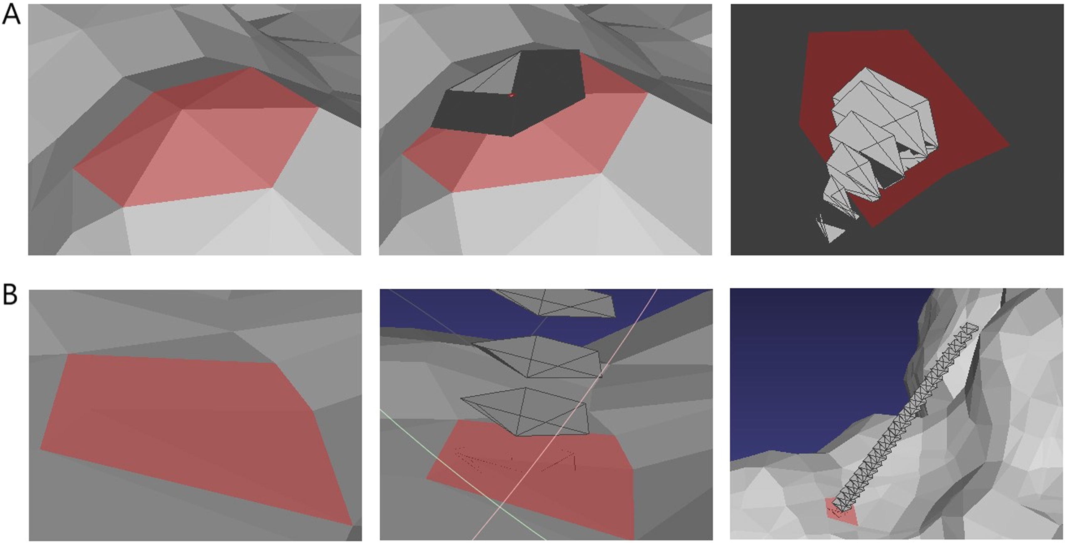
For a given protein with a PDB structure, we first performed protonation using Reduce (Word et al., 1999), then triangulated protein surfaces using the MSMS program (Sanner et al., 1996). Protein meshes were down-sampled and regularized by PyMesh (Zhou, 2018). In this way, the protein surface consisted of n meshes. The measurement of the concave–convex properties of the protein surface is as follows.
As is shown in Figure 1, for a given point O on the protein, we create a mesh object by the “form_mesh” function from the PyMesh library, and use the attribute “vertex_normal” that comes with the mesh object to get its normal vector V, so that we can represent the tangent planewith O and V. From the above step 2, we can obtain n triangular meshes which contain the point O. For each mesh For each mesh and barycenter, there is a point of intersection with tangent plane S. Assuming that each intersection is The n intersections and the given point O can enclose a polygon It is worth noting that in the PDB data, every amino acid contains many points (atoms), both of them need to be calculated. Then, in order to obtain the AoD of an amino acid, the AoD of convex and concave were both divided into 4 bins: Convex bins: Concave bins: If a point has the value of AoD between [−0.001, 0.001], we think it is a flat surface. We calculate the AoD of all points belong to the same amino acid, and for each bin, we collect the AoD at all points in that range. Thus, for AoD, we get a 9-dimension vector to describe. The MD was described in the same way but the number of bins and the range of each bin were different (10 bins). Besides the concave–convex feature we proposed, we also used Gaussian curvature and Mean curvature to describe the convex and concave properties of protein surfaces. Gaussian curvature is the product of the curvatures at a point on a surface, and the average curvature is Mean curvature. They can both be used to describe the shape of a surface at a certain point, such as convex and concave, and Mean curvature can even describe the trend of curvature change at that point. Based on the positive or negative value of curvatures, the shape of the surface at that point can be determined, such as convex, concave, cylindrical, and hyperbolic (Besl and Jain, 1988). For example, when Gaussian curvature is positive, a positive Mean curvature indicates that the surface is convex at that point, a negative Mean curvature indicates that the surface is concave at that point, and a zero Mean curvature indicates that the surface is conical at that point. According to Gaussian curvature and Mean curvature at a point on a surface, the shape of the surface can be determined. All possible cases are listed in Table 2. Therefore, an 8-length vector obtained based on Gaussian curvature and Mean curvature on the surface is used to describe the concave–convex features of the surface. And in the last, we add a dimension to represent the unknown concave–convex feature. Thus, we totally used a 28-dimension vector to describe the concave–convex feature.

Measurement of geometric feature of a point on an amino acid (the thick dotted lines with arrow represent the normal vectors (MNVs) of the meshes, then a polygon (S1) is formed by the intersections of these normal vectors with the tangent plane (S) of the point (O), and the intersection of the thin dotted lines represents the barycenter (BC) of a mesh).
Details of Convex and Concave Properties
As shown in Figure 3, the sequence and structural features of the protein are used as inputs to the prediction model. In this prediction model, it can be seen that the input features include Seq_Feature and Struct_Feature, which is constructed by different approaches. The common way to construct local protein features is usually based on protein sequence positions using sliding windows, and the Seq_Feature is constructed in this way. The method of constructing input feature through sliding windows enables the model to focus on local features of the sequence, but does not integrate well with structural features. Therefore, a method of the Struct_Feature for constructing local protein features based on protein spatial distance was proposed, with the following construction steps. (1) According to the PDB file of a protein, the coordinates of the atom of each amino residue are acquired and the Euclidean distances between all residue pairs are then calculated. (2) Choosing a Dcutoff. If the distance between residue pairs is less than or equal to the Dcutoff, this residue pairs will be chosen to construct the protein local features. On the contrary, if the distance between residue pairs is greater than the Dcutoff, this residue pairs will not be chosen.
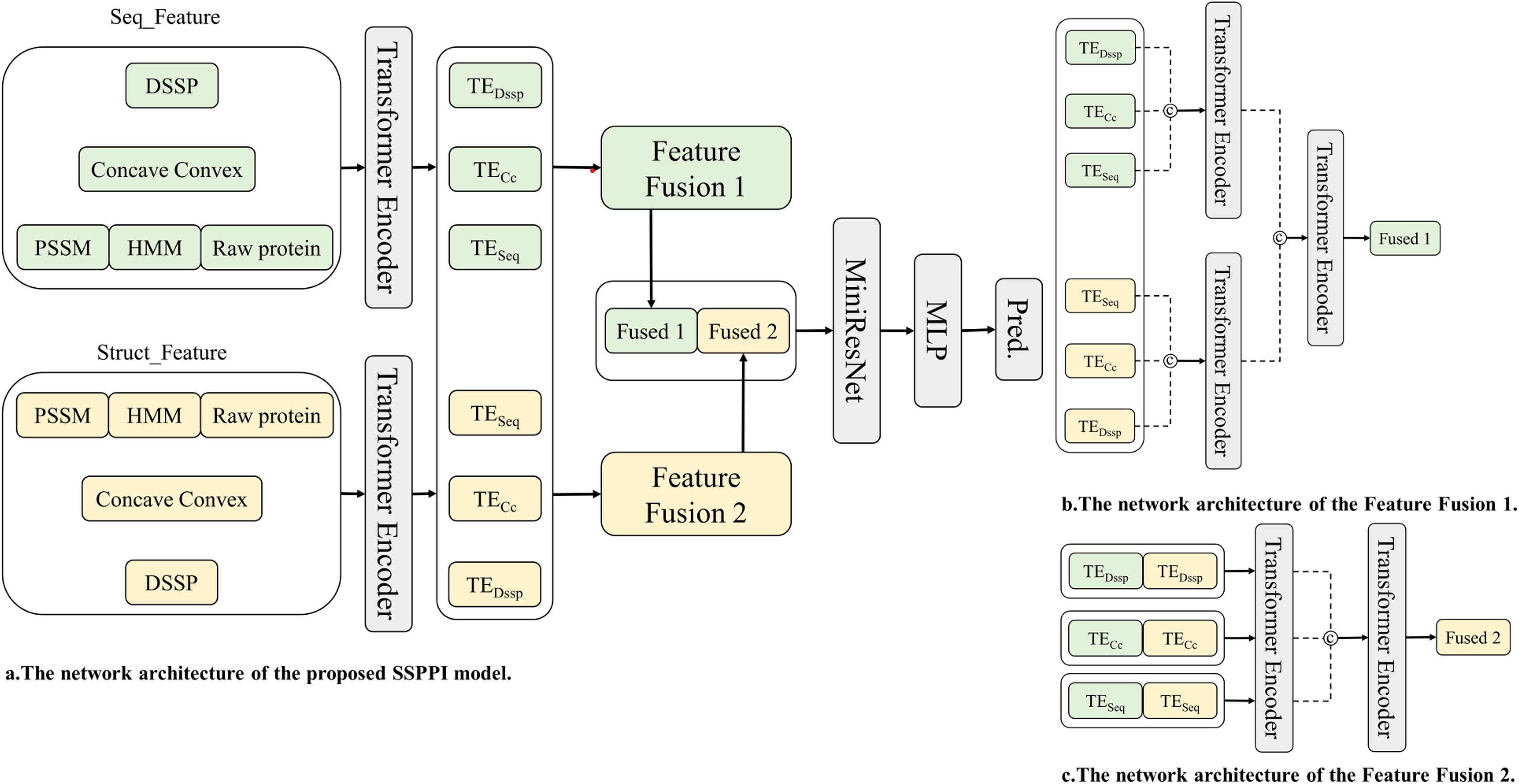
The network architecture of the proposed SSPPI model and the Feature Fusion model. SSPPI, Sequence and Structure geometric feature-based PPI site prediction.
In Figure 3, there were two different local feature fusion methods. The difference between them is when the Seq_Feature or the Struct_Feature is fused. In the Feature Fusion 1, the local feature will be further extracted before fusion. On the contrary, in the Feature Fusion 2, the same type of features within different local features will be fused firstly, and then the different types of features be fused secondly.
Particularly, in order to enable the model to focus on the positional features of the corresponding amino acids in the protein sequence, Position-index is added to the sequence feature in the Seq_Feature:
The Transformer Encoder (Fig. 4) is used to add attention mechanisms to both sequence and structural features. Input features are linearly transformed to generate the Q, K and V vectors, which are then split into n heads and each head has its own set of linear transformation parameters. For each head, a scaled dot-product attention is computed. Specifically, the product of Q and K matrices is calculated, scaled, and passed through the softmax function to derive the attention weights. These weights are then applied to the V matrix to obtain the attention output for each head. Finally, the outputs from all heads are concatenated and linearly transformed to produce the final attention result. The first use of the Transformer Encoder is to extract attention within features. For DSSP, Concave Convex and [PSSM, HMM, Raw protein] in the Seq_Feature or the Struct_Feature, every feature has a separate Transformer Encoder and is used to extract
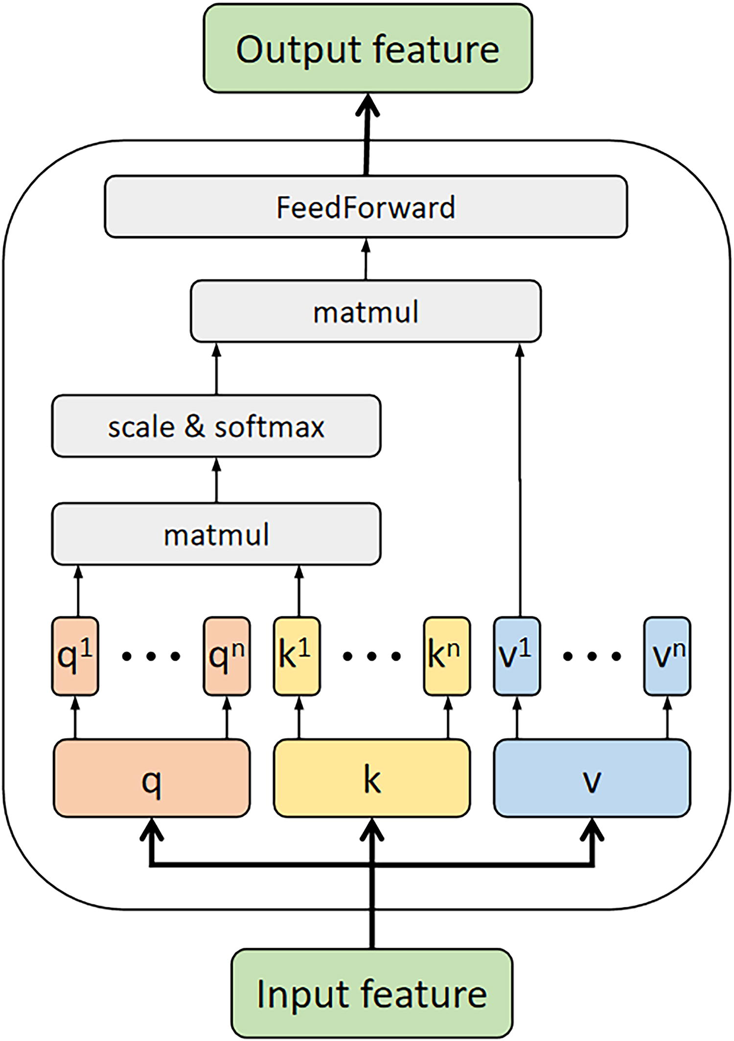
Transformer Encoder.
Parameters Used in SSPPI
The parameters are divided into four groups: the first three groups are the Transformer Encoder parameters for each feature ([PSSM, HMM, Raw protein], DSSP, and Concave Convex), while the last group consists of the training hyper-parameters.
HMM, Hidden Markov Models; PSSM, Position-Specific Scoring Matrices; DSSP, Dictionary of Secondary Structure in Proteins; SSPPI, Sequence and Structure geometric feature-based PPI site prediction.
We implemented our model with Paddle 2.2.2, with the following set of hyper-parameters: learning rate of 0.001, weight decay of L2Decay with 0.005 and the dropout rate of 0.1 to avoid over-fitting. We employed Focal Loss function (Lin et al., 2020) and AdamW optimizer for optimization. Detailed parameters are shown in Table 3. Focal Loss was calculated using the equation below:
The training process lasted at most 100 epochs and took approximately 26 seconds for every epoch on a NVIDIA Tesla A40 48G GPU.
Similar to previous studies, 9 evaluation metrics were used in our work: accuracy (ACC), precision (PRE), sensitivity (SEN), specificity (SPE), Recall, F-measure (F1), Matthews’ Correlation Coefficient (MCC), area under the receiver operating characteristic curve (AUROC), and area under the precision-recall curve (AUPRC) to evaluate the predictive performance of the models.
These metrics were calculated based on a threshold to convert predicted interacting probabilities to binary predictions. Therefore, it is necessary to use threshold-independent metrics, such as AUROC and AUPRC, to revealing the overall performance of model.
Comparison of methods for constructing local features
In this study, two methods for constructing local features of proteins are utilized: sliding windows based on protein sequences and spatial distance relationships based on protein structures. To determine the most appropriate sliding window length and spatial distance Dcutoff for constructing local protein features, various experimental combinations were established by adjusting these parameters. The sliding window sizes were set to 1, 3, 5, …, 19, resulting in a total of ten groups. For each set of experiments, the spatial distances Dcutoff were set to 4, 5, …, 15, forming a total of 12 groups. Additionally, comparative experiments were conducted to evaluate the local feature construction using only the sliding window method and only the spatial distance relationship method. The training set is Train_355, and the test set is Dset_60.
To maintain consistency and mitigate the influence of changes in parameter count on experimental outcomes, the model depicted in Figure 3 exclusively utilizes sliding windows to generate local features, constructing only Seq_Feature. To ensure consistency in parameter count, the Struct_Feature component of the model has been replaced with Seq_Feature. Similarly, this modification has been implemented in the model that relies exclusively on spatial distance relationships to construct local features.
Supplementary Table S1 shows the performance of predictive models under different Dcutoff when the window size is set to 1. Supplementary Tables S4, S5, S6, S7, S8, S9, S10, S11 and S12 shows other different window size’s results. Based on the data in the table, we can infer that when the window size is 1 and the spatial distance is 7, the prediction model achieves optimal performance, excelling in all performance metrics. Supplementary Table S2 shows the experimental results of using only the sliding window to construct local features. Supplementary Table S3 show the experimental results of using only the spatial distance relationship to construct local features.
For a prediction model that constructs local features using only a sliding window, performance reaches its peak when the window length is 15. For a prediction model that constructs local features using only spatial distance relationships, performance is best in threshold-independent metrics such as AUROC and AUPRC when the spatial distance Dcutoff is 14. In terms of the threshold-related comprehensive evaluation metrics, F1 and MCC decreased by 0.002 each compared to the prediction model with a spatial distance Dcutoff of 15, but the difference is not significant.
To investigate the impact of window length and spatial distance on model performance, the average model performance for all spatial distances at each window length is calculated and compared with the model that solely utilizes sliding window-constructed localized features. Similarly, the average model performance for all window lengths at each spatial distance is calculated and compared with the model that uses only spatial distance-constructed localized features. The results are shown in Figures 5 and 6.

Comparison of average performance under different window lengths (short dashed line) and performance using only sliding windows to construct local features (long dashed line).
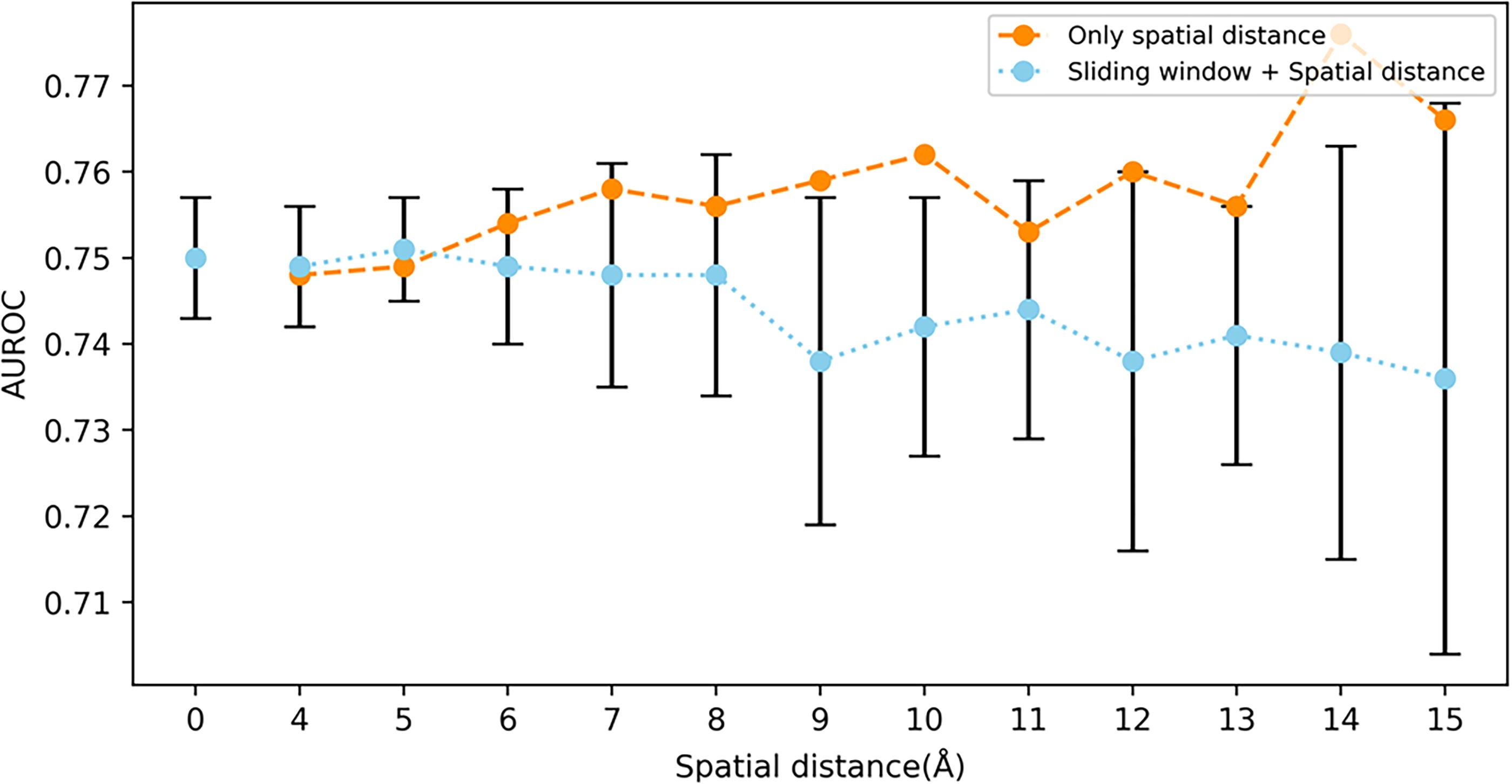
Comparison of average performance under different spatial distances (short dashed line) and performance using only spatial distance to construct local features (long dashed line).
As shown in Figures 5 and 6, the short dashed line points represent the mean of the model performances, and the black points denote the standard deviations. The long dashed line depict the performance curves when using only a single type of local feature (either sliding window on the sequence or spatial distance). In Figure 5, the mean and standard deviation at a window length of 0 represent the model’s performance when local features are constructed solely based on spatial distance, without utilizing sliding windows. For the model that uses only sliding window-constructed local features, its performance peaks at a window length of 15. When the window lengths are 1 and 3, combining spatial distance-constructed local features significantly enhances the model’s predictive performance. However, for window lengths greater than 3, combining spatial distance-constructed local features leads to a decrease in predictive performance. In Figure 6, for the model that uses only spatial distance to construct local features, the optimal performance is achieved at a spatial distance of 14. At spatial distances of 4 and 5, incorporating local features constructed from the sequence sliding window slightly improves the model’s prediction performance. Conversely, for spatial distances greater than 5, combining local features from the sequence sliding window reduces the model’s prediction performance.
The PPI site prediction model in this study is based on both sequence and structural features of proteins. To demonstrate the relative importance of each adopted feature, we conducted eight groups of feature ablation experiments: using only the sequence feature group (Sequence), using only the structure feature group (Structure), removing only the protein PSSM feature group (-PSSM), removing only the protein HMM feature group (-HMM), removing only the protein raw amino acid sequence feature group (-Raw Protein), removing only the protein secondary structure characterization group (-DSSP), removing only the protein molecular surface concave–convex characterization group (-concave–convex), and using all characterization groups (SSPPI).
To better evaluate the performance of each group, we performed 5-fold cross-validation on the Train_355, where the data were split into five folds randomly. Each time, a model was trained on four folds and evaluated on the remaining one fold. This process was repeated five times, and the AUROC and AUPRC scores on the five folds were averaged as the overall validation performance.
The results of the feature ablation experiments are shown in Table 4. The performance using the structural feature group is better compared to that using the sequence feature group, indicating that structural features such as secondary structure and molecular surface concave–convex features are more directly relevant to the identification of PPI sites. Interestingly, the performance without the protein secondary structure features is almost identical to the performance without the protein molecular surface concave–convex features. However, the performance using all feature groups is better than using either of these groups alone, suggesting that these two features have a potential complementary relationship in predicting PPI sites.
Results of Ablation Experiment
Results of Ablation Experiment
AUPRC, area under the precision-recall curve; AUROC, area under the receiver operating characteristic curve.
For the predictive model that combines local features constructed using sliding windows and spatial distances, its prediction performance does not show a significant improvement compared to models using a single type of local feature construction method (either using only sliding windows or only spatial distances). The specific results of each type of feature model on Dset_60 were analyzed. Table 5 shows the best performance for each type of feature model: SSPPI, which combines local features constructed using sliding windows and spatial distances, with a sliding window length of 1 and a spatial distance of 7; Sequence, which uses only sliding windows to construct local features, with a sliding window length of 15; and Structure, which uses only spatial distances to construct local features, with a spatial distance of 14. Although SSPPI achieves the best performance in all metrics, it does not show a significant improvement compared to the other two feature models.
The Optimal Performance of Various Types of Feature Models
The Optimal Performance of Various Types of Feature Models
ACC, accuracy; PRE, precision; SEN, sensitivity; SPE, specificity; F1, F-measure; MCC, Matthews’ Correlation Coefficient.
The bold numbers in the table represent the best results for each metric from different feature models.
Supplementary Table S13 shows the test results of various feature models on a subset of proteins in the test set. It can be observed that SSPPI does not achieve the best prediction results for all proteins. In the Dset_60, the SSPPI feature model achieves the best prediction results for 20 proteins, while the Sequence feature model achieves the best results for 16 proteins, and the Structure feature model for 24 proteins. Additionally, the results indicate that for proteins where SSPPI performs the best, such as 1e96_B and 1g14_A, the local features in the sequence and spatial domains complement each other, thereby enhancing the model’s performance. Conversely, for proteins where SSPPI performs the worst, such as 1ggp_A, 1gla_G, and 1qa9_A, the interaction between the two types of features may negatively affect the model’s performance. Therefore, besides constructing models that combine sliding window and spatial distance features for prediction, it is also beneficial to combine the prediction results from models that use only sliding window features and models that use only spatial distance features. Based on this, an ensemble model based on multiple local features is proposed. This model combines the predictions from different local feature models to achieve optimal predictive performance, as illustrated in Figure 7. Specifically, the parameters of each local feature model are fixed and not updated during the training of the ensemble model. The input to the ensemble model is the output from the penultimate fully connected layer of each type of prediction model (the last fully-connected layer is 32 × 1, which outputs the prediction probability; the penultimate layer is 128 × 32), and that is concatenated with the sequence length of the protein and then is used as input to MLP.

An ensemble models based on multiple local features.
The training parameters and environment of the ensemble model are consistent with those described in Figure 3, and the final results of this model are described in Table 5. The performances of the ensemble model, compared to SSPPI, in the five metrics of AUROC, AUPRC, Recall, F1 and MCC, increase from 0.776, 0.394, 0.414, 0.413 and 0.303 to 0.801, 0.432, 0.533, 0.459 and 0.345, obtaining a 3.222%, 9.645%, 28.744%, 11.138% and 13.861% improvement respectively, and the performance of the ensemble model has indeed improved.
Supplementary Figures S1 and Figure S2 show the AUROC and AUPRC results for each type of feature and the ensemble model, with the ensemble model exhibiting a significantly improved performance compared to the other three models.
We compared SSPPI_Ensemble with five sequence-based predictors, PSIVER (Murakami and Mizuguchi, 2010), ProNA2020 (Qiu et al., 2020), SCRIBER (Zhang and Kurgan, 2019), DLPred (Zhang et al., 2019), and DELPHI (Li et al., 2021), and four structure-based predictors, DeepPPISP (Zeng et al., 2020), SPPIDER (Porollo and Meller, 2007), MaSIF-site (Gainza et al., 2020), and GraphPPIS (Yuan et al., 2021). Note that our test sets may be part of the training sets in other methods. If true, the results reported here would be upper limits for other methods.
As shown in Table 6, there is a large performance gap between SSPPI_Ensemble and the five sequence-based methods. The most likely reason is the lack of structural features in these sequence-based methods. As discussed in Section 3.3, the prediction model requires different features for different proteins. For example, by using the combination of different features, SSPPI_Ensemble improves over DELPHI by 14.592%, 35.423%, 23.387%, and 53.333% in AUROC, AUPRC, F1 and MCC. In comparing with four structure-based predictors, we pay more attention to MaSIF-site and GraphPPIS, and the former is based on point cloud geometric neural networks, while the latter is based on graph convolutional neural networks. These two predictors can automatically calculate protein spatial features, so the comparison with them better demonstrates the effectiveness of the structural features proposed in our study. The difference between our model and MaSIF-site is whether the local features are constructed or not. MaSIF-site constructs the geometric features and the chemical features, and takes the entire protein as input. Our model constructs local features based on protein sequence and spatial distance. SSPPI_Ensemble outperforms MaSIF-site in ACC, PRE, F1, MCC and AUROC, but is slightly worse than MaSIF-site in AUPRC and Recall. This indicates that through the local feature construction method proposed in this study, the predictors may learn the global features of proteins. GraphPPIS constructs the PSSM, HMM and DSSP features, and uses the adjacency matrix to choose the input amino acid residue. SSPPI_Ensemble outperforms GraphPPIS in ACC, PRE, AUROC, AUPRC, F1, and MCC, which indicates that the molecular surface concave–convex features proposed in this study as a structural feature can effectively improve the performance of predictors.
The Optimal Performance of Various Types of Feature Models on Dset_60
The Optimal Performance of Various Types of Feature Models on Dset_60
Predictions by the programs marked with * were cited from Yuan et al. (2021). Predictions by PSIVER, ProNA2020 and SPPIDER were directly generated from their web servers. ProNA2020 only makes binary predictions and thus, the AUROC and AUPRC are not calculated. The Performance of SSPPI_Ensemble is based on Train_335. The bold numbers in the table represent the best results for each metric from different models on Dset_60.
ROC and PR curves for the tests sets
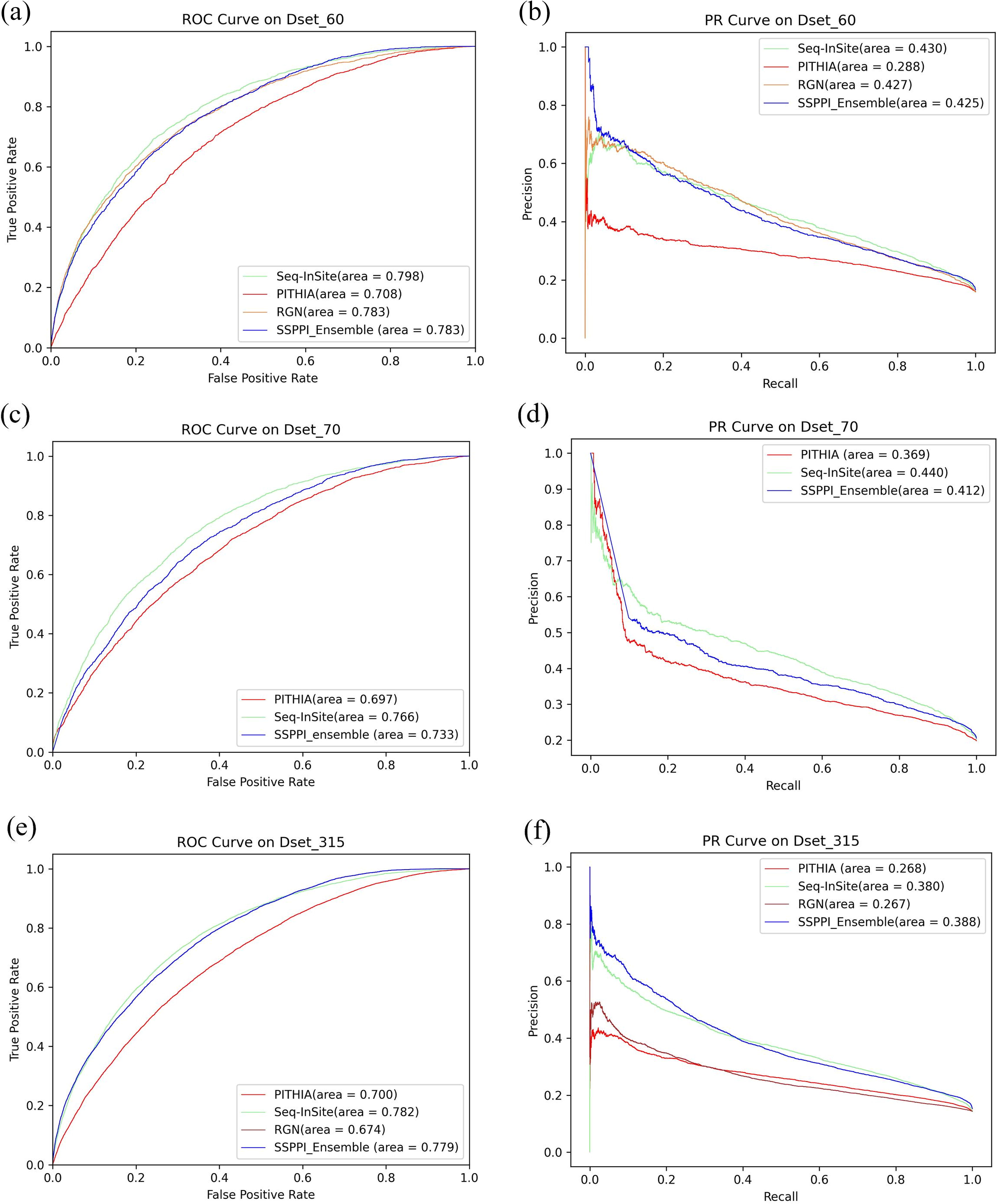
To further validate the performance of SSPPI_Ensemble, we applied the model to our newly constructed datasets, which include the updated protein sequences and interactions. As shown in Table 7 and Figure 8, our method, SSPPI_Ensemble, demonstrates its advantages over other methods across three test datasets. Although it performs slightly worse than Seq_InSite (Hosseini et al., 2024) in some metrics, the overall advantages is obvious. In Dset_70 dataset, SSPPI_Ensemble achieves the best performance in three key metrics: SPE (specificity), PRE (precision) and ACC (accuracy), with values of 0.921, 0.463, and 0.789, respectively, which surpass Seq_InSite’s performances of 0.864, 0.447, and 0.781.
The Optimal Performance of Various Types of Feature Models on Different Test Datasets
Predictions by the programs marked with * were cited from Hosseini et al. (2024). The Performance of SSPPI_Ensemble is based on Train_1326. The bold numbers in the table represent the best results for each metric from different models on three test datasets.
On Dset_315 dataset, SSPPI_Ensemble achieves the highest AUPRC score of 0.388, outperforming Seq_InSite, PITHIA (Hosseini and Ilie, 2022), and RGN (Wang et al., 2022) by 2.105%, 44.776%, and 45.318%, respectively. For other metrics, our method is nearly equivalent to Seq_InSite, with the SEN values of 0.395 versus 0.398, the SPE values of 0.898 versus 0.899 and the ACC values of 0.827 versus 0.827. Furthermore, SSPPI_Ensemble significantly outperforms PITHIA and RGN across all metrics. For instance, SSPPI_Ensemble’s MCC value of 0.292 is notably higher than PITHIA’s 0.184 and RGN’s 0.185, further confirming the effectiveness of our approach.
These results highlight the power of the proposed structural three-dimensional point cloud concave–convex feature in capturing PPI site information, and the features is particularly effective in revealing surface shape variations and identifying potential binding sites. By integrating sequence context information and spatial distance relationships between amino acids, our ensemble model enhances the prediction performance of PPI sites.
Predicting PPI sites is very important for understanding the function of proteins. In this study, we combined sequence feature (PSSM, HMM and Raw protein sequence) and the structure feature (DSSP and concave–convex) to predict PPI sites. And the most important is that we proposed a novel method to calculate the geometrical features of amino acids based on the concave–convex properties of protein surface. We measured the degree of concave–convex by moving the tangent plane at a point of an amino acid, and examining the change rate of the polygon area formed by the intersections of the plane and the normal vectors on the triangular mashes of the point. Combining these two types of features, using the Transformer-encoder, mini-Resnet, and the proper ensemble methods, a novel prediction module, SSPPI_Ensemble, was proposed. Comparing with the state-of-the-art method, we obtained better prediction results or results with significant advantages, to which structure features make a significant contribution. From the ablation experiments, we found that the concave–convex feature can make the same contribution with the DSSP to the performance. Prediction of PPI sites is still a challenging task. It is necessary to introduce more features (such as co-evolution) or create novel features, to further improve the prediction performance.
Footnotes
ACKNOWLEDGMENTS
The authors thank Professor David R. Westhead (Leeds University, UK) for his valuable comments and useful suggestions on the revision of this article and Professor Fuyi Li (Northwest A&F University, China) for making some corrections to the grammar of this article.
AUTHORS’ CONTRIBUTIONS
L.L. and J.G. performed conceptualization, data curation, software development, formal analysis, and writing. H.D. conducted part of investigation and S.C. joined part of writing. J.Y. and L.H. provided conceptualization, methodology, writing, and supervision.
AUTHOR DISCLOSURE STATEMENT
The authors declare they have no conflicting financial interests.
FUNDING INFORMATION
This work was supported by
References
Supplementary Material
Please find the following supplemental material available below.
For Open Access articles published under a Creative Commons License, all supplemental material carries the same license as the article it is associated with.
For non-Open Access articles published, all supplemental material carries a non-exclusive license, and permission requests for re-use of supplemental material or any part of supplemental material shall be sent directly to the copyright owner as specified in the copyright notice associated with the article.