The growing volume of genomic data, driven by advances in sequencing technologies, demands efficient data compression solutions. Traditional algorithms, such as Lempel-Ziv77 (LZ77), have been fundamental in offering lossless compression, yet they often fall short when applied to the highly repetitive structures typical of genomic sequences. This review explores the evolution of LZ77 and its adaptations for genomic data compression, highlighting specialized algorithms designed to handle redundancy in large-scale sequencing datasets efficiently. Innovations in this field have enhanced compression ratios and processing efficiencies leveraging intrinsic redundancy within genomic datasets. We critically examine a spectrum of LZ77-based algorithms, including newer adaptations for external and semi-external memory settings, and contrast their efficacy in managing large-scale genomic data. We conducted experiments to evaluate the performance of several algorithms, including KKP2, RLE-LZ, SE-KKP, BGone, and PFP-LZ77, on both real-world datasets from the Pizza&Chili repetitive corpus, Salmonella genomes, and human chromosome 19 genomes. These results underscore the trade-offs between time and memory consumption between algorithms. This article aims to provide a comprehensive guide on the current landscape and future directions of data compression technologies, equipping bioinformaticians and other practitioners with insight to tackle the escalating data challenges in genomics and beyond.
INTRODUCTION
In the era of increasingly larger datasets, the exponential growth of genomic data generated by advanced sequencing technologies poses significant challenges to data storage and management. The vast amounts of data produced are not only massive in scale, but also exhibit a high degree of redundancy, particularly within and between genomes of the same species (Lukens et al., 2004). This redundancy, while beneficial for data compression, demands sophisticated algorithms to efficiently leverage these repetitive structures for improved storage and retrieval processes.
To address these challenges of managing large and redundant datasets, bioinformatics has turned to compression algorithms that can effectively exploit repetitive structures in genomic data. One of the foundational methods in this area is LZ77- , which is a seminal lossless data compression algorithm developed by Abraham Lempel and Jacob Ziv. 77 laid the foundation for numerous modern compression techniques. Published in 1977, 77 employs a sliding-window mechanism to find repeated sequences within a fixed-size window, encoding data as a triple (distance, length, and next symbol). The distance in the tuple refers to how far back the encoder must look within the sliding window (the buffer of previously processed data) to find a matching substring. The length indicates how long the matching substring is, providing the decoder with information on how many characters to copy from the position identified by the distance. Finally, the next symbol is the character that follows the matched substring or the character itself when no match is found. This character represents the starting character of the new 77 phrase, allowing us to continue processing beyond the matched part when we want to decode the sequence. This method allows 77 to efficiently compress data by encoding repeated substrings using references to earlier parts of the string rather than storing them explicitly. For example, the string abcabcabcabc encodes the following series of tuples: (0, 0, a), (0, 0, b), (0, 0, c), (3, 3, a), (3, 3, a).
In this review, we trace the evolution of 77 algorithms, focusing on innovations that make them suitable for large-scale genomic datasets. Designed for readers new to data compression, this work introduces methods based on 77 that address the substantial redundancy and volume characteristic of genomic data, which often contains repetitive elements, especially within species. Efficient compression is crucial for managing the data produced by modern sequencing technologies, and 77 has become a versatile tool in bioinformatics. For example, Wertenbroek et al. (2022) use 77 to develop a genotype compression tool for large biobank data. Norri et al. (2021) used it to develop a method to identify structural variants from multiple alignments. The tools that use 77 have been evaluated for their use for taxonomic identification in metagenomics (Silva and Almeida, 2024). It has also been used for read data compression sequencing (Kowalski and Grabowski, 2020; Castelli et al., 2024). With such varied applications, a wide range of 77 algorithms warrants exploration. We also highlight advancements in hardware implementations of 77, which address throughput challenges inherent to software-only approaches, enabling faster data processing and supporting real-time genomic analysis. Table 1 summarizes the representative 77 algorithms discussed in this review, comparing their complexities in time and space.
Illustration the Time and Space Complexity for in Memory Construction Algorithm
Algorithm
Time complexity
Space complexity
factorization by Peak Elimination (Ohlebusch and Gog, 2011)
136n bits
Ultra-Fast Lempel-Ziv77 (77) factorization (Ohlebusch and Gog, 2011)
104n bits
77 factorization backward search (Ohlebusch and Gog, 2011)
40n bits
Lazy LZ Construction (Kempa and Puglisi, 2013; Goto and Bannai, 2013)
The symbol represents the alphabet, n corresponds to the length of the input, and r is equal to the number of maximal single-character runs in the BWT. For algorithms where experimental space usage was reported in the original articles, we present those measurements. Otherwise, we list the theoretical space bounds.
To assess the practical impact of these advances, we conducted a series of experiments to validate the performance of various 77-based algorithms in the management of large-scale genomic data. We evaluated the performance of KKP2, RLE-LZ, PFP-LZ77, and SE-KKP, while KKP1 and KKP3 were excluded due to their inability to support large datasets. Although we reached out to the authors of the LZone algorithm, we were unable to access the source code, and there is currently no available implementation for the sublinear 77 algorithm. SE-KKP was selected to represent external memory 77 construction, given its demonstrated superior performance in external memory settings in a previous benchmark study. The experiments used real-world datasets from the Pizza&Chili corpus and Salmonella genomes obtained from the NCBI website.
Our results on the Pizza&Chili corpus revealed that all algorithms, except RLE-LZ, required less than 5 GB of memory and were completed in 20 minutes, with RLE-LZ consistently taking the longest time but consuming the least memory. SE-KKP consumed the most memory and time in various scenarios, while KKP2 and PFP-LZ77 performed similarly in terms of both time and memory. For Salmonella data sets, KKP2 was the fastest algorithm, and RLE-LZ, despite using the least memory, failed to complete within the 24-hour time limit for the largest data set. These findings underscore the trade-offs between time and memory efficiency in all algorithms tested.
Through a comprehensive examination of 77 factorization algorithms, this article aims to provide a detailed guide on the current state of the art and future directions in this field. Our objective is to equip researchers and practitioners with the knowledge and tools necessary to tackle the challenges of genomic data management, paving the way for more efficient and effective use of genomic information in various biological and medical applications.
NOTATION AND PRELIMINARIES
Basic definitions
We denote a string S as a finite sequence of symbols over an alphabet whose symbols have a total order. We denote by the empty string. We define the length of S as the number of characters and denote it by | S |. Given a string S, we denote the reverse of S as , that is, . Lastly, we define the rotation of a string as a transformation in which the characters of the string are shifted circularly such that some characters at the beginning of the string are moved to the end. Formally, for a string S of length n, the i-th rotation of S is the string for 1 .
We denote by the substring of S starting at position i and ending at position j, with if . For a string S and , is called the i-th prefix of S, and is called the i-th suffix of S. We call a prefix of S a proper prefix if . Similarly, we call a suffix of S a proper suffix if .
We denote by < the lexicographic order: for two strings and , if S is a proper prefix of T, or if there exists an index such that and .
Rank and select
Given a string S of length n, a symbol , and an integer i, we define as the rank, as the number of occurrences of c in . We also define as the position in S of the i-th occurrence of c in S if it exists and otherwise. For a bitvector , that is, a string over , to simplify the notation, we will refer to and respectively as and .
The operations and efficiently count and locate repeated substrings, which accelerates LZ77’s process of replacing these substrings with references to their previous occurrences.
Burrows–Wheeler transform
The Burrows–Wheeler transform () (Burrows and Wheeler, 1994) of a string S is a reversible permutation of the characters of the string S. This transform is obtained by sorting all rotations of a string S in lexicographic order and retaining the last character of each rotation. Let M be the matrix containing all sorted rotations of S, let F and L be the first and last columns of the matrix, then . Moreover, let be the number of suffixes starting with a character smaller than c, where c is in . We define as the number of occurrences of character c in the substring and define LF-mapping (Burrows and Wheeler, 1994) as and . LF-mapping can be used to count the occurrences of a pattern P in S. We refer to this technique as backward search. We note that when it is clear from the context, we remove the subscript in the notation, that is, is denoted as
Given a string S and its BWT, a run in BWT is a maximal substring of equal characters in BWT. This leads to the definition of the run-length encoded Burrows–Wheeler Transform () (Mäkinen and Navarro, 2004), which offers a more space-efficient variation by compressing sequences of repeated characters in the sequence into a single run. Again, when it is clear from the context, we remove the subscript in the notation, i.e., is RLBWT. Hence, RLBWT is an equivalent representation of BWT, where each run is represented as the character of the run and its length. For example, given the of string S as bd#bbbbddddbaaaaaaaaaaa, the sequence of characters beginning each run is described as bd#bdba. Each character c in S has its run lengths encoded in a corresponding bitvector , with a 1 marking the start of each run. In this case, the bitvectors are , , , , and . Hence, we note that denotes the location of the start of each run in S, and the character bit vectors denote the start and length of the runs for each character. The rank and access operations are efficiently translated into the rank, select, and access operations in H, , and for all characters c. This encoding strategy reduced the storage of to , where r denotes the number of runs in the , since there exists a constant number of 1 bits for each run in this encoding.
Suffix array and inverse suffix array
The suffix array (Manber and Myers, 1993) () is a compact and efficient data structure that implicitly stores all the sorted suffixes of a string S of length n. More specifically, we note that the for the string S is a permutation of such that represents the i-th lexicographically smallest suffix of S. Relating this back to our definition of , this is the starting position of each of the rotations in the matrix M.
Complementing the is the inverse suffix array, we denoted it as . This serves as a mapping back to the lexicographical ranks of the suffixes, allowing one to determine the rank of each suffix in the lexicographical order efficiently. More formally, we find that is defined so that for all . We remove the subscript from the notation when it is clear from the context, i.e., is and is . The suffix array can help improve the efficiency of 77 compression, as follows for the rapid identification of repeated substrings, which 77 replaces with references to earlier positions in the string.
Longest common prefix array
Given two strings and , we refer to the longest common prefix as the substring such that and denote this by . Next, we define the longest common prefix () array as the data structure that stores the lengths of the longest common prefixes between consecutive suffixes in the of a string S. More specifically, represents the length of the longest common prefix between the suffixes represented by and in S, i.e., . When the context is clear, we remove the subscript from the notation. The can accelerate the process of 77 by precomputing and storing the length of common prefixes between consecutive suffixes, optimizing the search for the longest match.
Longest common extension
The longest common extension () array measures the length of the longest common prefix between two suffixes of a string S. Given the indices i and j, is the length of the longest common prefix of the suffixes starting at position i and j in S.
Range minimum query
Given an array of integers and an interval , a range minimum query (RMQ) of the interval [i, j] over the array , denoted by , returns the position k of the minimum value in . Formally, . The is frequently used with to answer questions such as: Given two suffixes and of the string , find the value of . This is achieved efficiently by performing an on the array, as described by Kasai et al. (2001). This can be done using over . Hence, given two integers we define as the longest common prefix between the i-th and j-th suffix in order, which is equivalent to computing the of and . Formally, the length of can be computed as (Kasai et al., 2001).
2.8. and
Given a string S[1, . . , n] and its and , the and are defined to facilitate efficient traversal of lexicographically adjacent suffixes. The array maps each suffix to the lexicographically previous suffix, for a suffix starting at position i, is defined as if , and otherwise (Kärkkäinen et al., 2009). The provides the position of the suffix that is lexicographically immediately smaller than the suffix .
In contrast, identifies the next lexicographic suffix. Formally, is defined as , with conditions and (Grossi and Vitter, 2005). This ensures that returns the position of the next lexicographic suffix following or 0 if no such suffix exists.
Previous smaller value and next smaller value queries
Previous smaller value (PSV) and next smaller value () queries are used frequently to calculate LZ77, as we will see within this survey. These queries concern themselves with an integer array and a specific index . The of at index i is defined as the maximum position preceding i within the array where there is a value smaller than . Formally
Similarly, of in the index i is defined as the minimum position succeeding i within the array where there is a value smaller than . Formally,
These queries find application in various algorithmic problems (Goto and Bannai, 2013; Kempa and Puglisi, 2013; Kärkkäinen et al., 2013a), particularly in tasks involving array traversal, range queries, and optimization problems. They are often used in algorithms to find the closest smaller element to the left or right for each element in an array.
Next, following the definitions provided by Kärkkäinen et al. (2013a), we introduce and which operate directly on :
and
Lastly, we define and as follows:
and
assuming = 0 for all . These last equations are used frequently to calculate the 77 factorization. We note that these text-based versions are essential for efficiently computing the 77 factorization, as they enable quick identification of the longest match by locating the nearest lexicographic neighbors in the suffix array. Using and queries, the search for repeated substrings is optimized, avoiding redundant comparisons.
The FM-index
The FM-index (Ferragina and Manzini, 2000) is an index based on the BWT and the SA. As we have seen, BWT is capable of counting the number of occurrences of a pattern by itself. In order to locate all such occurrences, SA is required. We note that, in order to achieve compression, the FM-index does not store all the SA values, instead, it samples some of the values while still being able to compute the values that are not sampled through the LF-mapping. As a result, the FM-index of a string S is capable of computing the number of occurrences of a pattern P in time, and can compute the positions of all occ occurrences in for by storing the BWT plus bits of auxiliary information, where n is the length of S. That is, to find a pattern P in the FM-index, we can use the LF mapping to find the range [sp, ep] of the BWT that corresponds to all the suffixes of S that are prefixed by P. Once we obtain the range on the BWT, we land, in the last LF step, on one of the sampled positions of the SA, or we have to retrieve it. To do so, we continue performing steps of the backward search until we find a value of the SA that is sampled. From that sample, we can compute the value of SA that we were looking for. The FM-index is a compressed full-text substring index that leverages the BWT to efficiently search for an input string S. The index uses the BWT to rearrange the original string, grouping similar contexts together for improved compressibility. To navigate and reconstruct the string, the FM-index employs rank and select structures, which efficiently count character occurrences up to any position in the BWT. Instead of storing the entire suffix array, the FM-index keeps sampled positions, aiding in quick location jumps within the string. One of its fundamental features, the backward search, allows the index to efficiently find substrings by analyzing from the end of the pattern to its beginning.
LZ77
Given a string , the 77 (Ziv and Lempel, 1977) factoring of S is a decomposition of S into z phrases . There are two types of phrases, literal phrases that are phrases representing the first occurrence of a character in S and repeat phrases that correspond to substrings that occurred previously in the string. The 77 phrases can be constructed inductively as follows. Assume that we already computed the first phrases of the factorization, and let i be such that . The next phrase is a literal phrase if S[i] never occurred in . Otherwise, the next phrase is the longest prefix of that occurs in S at position , i.e., with denoting the length of the repeated phrase. The 77 factorization can be compactly represented as a list of phrases where if is a literal phrase, we set and equal to the character S[i] never seen before in the string.
While the 77 factorization divides the string into nonoverlapping phrases, the concept of the longest previous factor (LPF) provides information about repetitions at every position in the string. For a position , the pair such that and , with maximized. This provides a compact way to capture the longest repeated substring starting at position i and occurring earlier in the string.
COMPUTING THE 77 COMPRESSION
In-memory construction of 77 involves managing a sliding window of data that efficiently encodes repeated substrings by referencing previous occurrences directly within memory. Here, we provide a concise overview of these in-memory construction algorithms, presented in chronological order.
Early methods of computing 77
Ohlebusch and Gog (2011) presented two algorithms in 2011 for computing 77 factorization. The first algorithm begins by computing the and in linear time. Next, two additional arrays are computed: the longest previous substring () and the previous occurrence position of the first appearance of each character (). The array stores the length of the longest prefix of the substring starting at position k that has occurred earlier in the string S, i.e.,
In other words, is the length of the longest prefix of that matches a substring appearing before position k. If no such prefix exists, then is equal to 0. The array stores the position j where occurs for each position k. More specifically, stores the position j such that and occur at that position j. If no such position exists, then is undefined.
The algorithm for computing these arrays is conceptualized using a graph-based representation of and , which was originally introduced by Crochemore and Ilie (2008). The graph has nodes, where there exists a node for every , where i is a position in SA, and nodes with labels and . Two nodes and are connected by an edge marked with . A peak in this graph occurs when and . After the construction of this graph, the peaks are then identified and eliminated to derive and values. Each peak is eliminated by removing the node and replacing it with a new edge labeled between and . For each eliminated peak node i, LPS and PrevOcc values are determined as follows: = . The value of is set to if . Otherwise, = if . After construction of the and arrays, the 77 factorization is computed using the array to find the length of the longest previous match at each position, while the array provides the starting position of this match. If no match is found, the current character is encoded directly.
This algorithm is further optimized by interleaving the computation with the peak elimination process. Instead of pre-computing the entire array, their enhanced version performs incremental computation while simultaneously processing potential peaks. This optimization reduces memory usage while achieving better runtime performance, especially for highly repetitive strings.
The second algorithm improves the space efficiency of the first algorithm by performing a backward search on of . The algorithm first constructs a for . From this , it derives the using the formula, and computes the Previous Greater Value () and Next Greater Value ()—instead of and —needed since the algorithm processes . The boundary cases are handled by setting , where
and
After constructing the of the and the and arrays, the 77 factorization is computed as follows. For each position k in S, the algorithm identifies an interval that contains suffixes that begin with the substring using a backward search in of . Then it checks if or falls within this interval. If neither nor falls within this interval, then it follows that S[k] has no previous occurrence, and the factor is outputted. However, if or falls within this interval, then it continues the process by extending the pattern to through backward search to get a new interval, and again checks if or falls within this new interval. This process continues until the maximum length substring, denoted as , is found such that the interval contains either or . The starting position p of the factor is then determined using the position corresponding to or . The algorithm outputs each 77 factor as a pair .
Lazy 77 construction
Kempa and Puglisi (2013) and Goto and Bannai (2013) independently developed algorithms to calculate 77 based on the knowledge that, given a position i in S, the new 77 factor can be found by comparing suffixes at positions and . In particular, the length of the 77 factor at position i can be determined by computing . Notably, both Kempa and Puglisi (2013) and Goto and Bannai (2013) only compute the and when i is the starting position of a phrase, and thus, are often referred to as “lazy evaluation” of values. The methods differ in the way and are computed. We now discuss each of these algorithms in detail.
Goto and Bannai define three linear-time algorithms that differ on the basis of their memory use. First, they define the BGT algorithm, which operates directly in text order, and use the array to maintain a mapping between each suffix and its preceding lexicographic suffix. Given the input string S of length n, this algorithm begins by computing and . With these structures in place, the algorithm then calculates and using the array, defined as for i greater than 0 and . Using this array, is assigned the value of if it exists; otherwise, it is set to 0. Meanwhile, is computed by scanning the array starting from position i. Once the values for and are calculated, the algorithm proceeds to determine the LPF for each position i in S using the expression . Finally, the 77 factors are constructed using the values. If is equal to 0, then the factor represents a new character at position i. Otherwise, the 77 factor consists of a reference to an earlier occurrence, with the position of the matching substring determined based on the computation of and . The algorithm then advances by characters. The BGT algorithm requires bits of space, making it the most memory-efficient algorithm among the three algorithms.
Next, they introduced the BGS algorithm that computes and using a stack. Similarly to BGT, this algorithm begins by computing the and . Next, it traverses the , computing the and using a stack. Subsequently, these values are converted to text order using , resulting in and . In particular, the transformations are defined by the equations: , and , Lastly, the 77 is computed in the same way as in the BGT algorithm. This algorithm is faster than the BGT algorithm but uses additional space. In particular, it requires bits of space, where s denotes the maximum size of the stack.
The third algorithm they introduced is BGL, which computes and without a stack, instead employing the peak elimination algorithm previously defined by Ohlebusch and Gog (2011). After this, the algorithm maintained the same computations as the BGS algorithm. The workspace required by BGL is .
The algorithm of Kempa and Puglisi begins by computing the and the for the input string S. The algorithm begins by constructing the predecessor () and successor () arrays using a stack and scanning the while maintaining a stack of positions. For each position i, the algorithm compares with , where j is the position that is at the top of the stack. If the stack is not empty and is greater than , then j is popped from the stack. This process is repeated until or the stack is empty. If the stack is not empty, then is equal to j. Otherwise, if the stack is empty, is equal to −1, indicating that there are no previous smaller suffixes. The index i is then pushed onto the stack, and the next position is considered. The array is computed in an identical manner, but the traversal of is in reverse order. Next, the algorithm uses the arrays , , , and to simulate and and calculate the factorization 77, with the property that for each position i, equals and similarly, equals . The next 77 factor is determined by identifying the longest previous match for the current position i, which is computed using and .
The KKP algorithms
Kärkkäinen et al. (2013a) introduced a suite of algorithms collectively called the KKP algorithms, named after the authors. Among these, the KKP3 algorithm requires bits of working space and shares close ties with the algorithms of Goto and Bannai (2013). KKP3 is a simple algorithm that the authors describe in 13 lines of pseudocode. It begins by first computing . After the is constructed, the and arrays are calculated using the approach of the BGS algorithm, i.e., using a stack and . After computing and , the 77 factors are calculated using lazy factorization, which is similar to the BGT algorithm described in Section 3.2. KKP3 does not construct or ; (2) KKP3 stores the arrays and in an interweaved manner so that and are next to each other, making access more cache efficient; and lastly, (3) is more memory efficient in the construction of and , that is, SA is overwritten by the elements of the stack, so only 2 arrays of size are ever stored in main memory.
KKP2 reduces memory consumption compared to KKP3. Instead of precomputing both and before computing the 77 factorization, KKP2 only precomputes the array. More specifically, given the string S, KKP2 starts by constructing , then computes using the same approach as KKP3, and stores the values of in the array , that is, , for each position i. Next, for each position t, KKP2 computes using and then determines the next 77 factor in the same way as KKP3 by comparing , , and t. This design ensures that both the values and can be retrieved directly from the array, eliminating the need for an additional array. By avoiding the precomputation and storage of , KKP2 reduces the working space to bits while maintaining linear time complexity.
KKP1 will be discussed in a later section, where external memory methods are discussed. The names of the methods, KKP3, KKP2, and KKP1, originate from the number of arrays (of length n) that are stored in memory. KKP3 stores SA, PSV, and NSV. KKP2 stores SA and . KKP1 assumes that SA is stored in external memory and only stores NSV in main memory.
The BGone algorithm
Motivated by the fact that the KKP algorithms store two arrays, Goto and Bannai (2014) developed algorithms to compute the 77 factorization using a single array. The name of the algorithm refers to the authors’ names and the number of auxiliary arrays used. They refer to their previous work that we described in Subsection 3.2 as BGtwo.
In order to describe BGone, we require some additional definitions. Given an input string S, we define the suffix to be either an S-type or an L-type based on lexicographical comparisons. A suffix is S-type if , or if and are S-type suffixes. Furthermore, is a L-type suffix if , or if and is a L-type suffix. Additionally, a suffix is defined as a Left-Most S-type (LMS) if it is a S-type and the suffix immediately preceding it is an L-type suffix.
Given a string S, BGone constructs the array using an algorithm that is similar to Nong (2013)’s induced sorting algorithm, which sorts a selected subset of suffixes (in this case, the LMS suffixes) and then uses their ordering to sort the remaining suffixes. Hence, the algorithm begins by scanning S from right to left and classifying each suffix as either L-type or S-type, initializing an auxiliary array A, and sorting the identified LMS suffixes lexicographically. This produces a lexicographically sorted list of LMS suffixes, which we denote as . These suffixes are then placed in alternating positions of the array A: specifically, for each i from 1 to k, we set , while the positions are left empty. Then, for each LMS suffix position and its lexicographic successor , the algorithm attempts to assign . If a value has already been assigned to —that is, if appears in the rearranged —the algorithm instead assigns . Once all assignments are complete, BGone performs two passes of induced sorting to incorporate all remaining suffixes into A: in the first pass, it incorporates all L-type suffixes in A, and in the second pass, it incorporates all S-type suffixes in A. After both passes are complete, the working array A is transformed into the array. Finally, BGone computes the 77 factorization using the array, following the same method as the KKP2 algorithm described in Subsection 3.3. By combining these in-place algorithms, Goto and Bannai present the first 77 factorization method that uses only a single auxiliary array of length n. The BGone algorithm runs in linear time and requires bits of space.
The LZoneT and LZoneSA algorithms
Building on the development of BGone, Liu et al. (2016) introduced the LZone algorithm, which maintains the same theoretical runtime and memory usage as BGone, but offers practical improvements in speed. Like BGone, it uses a single auxiliary array, but achieves better performance by more precisely handling L-type and S-type suffixes. This is achieved through a reorganization of the suffix sorting process to avoid unnecessary scans and random access operations. LZoneT begins by counting the number of L-type and S-type suffixes, then adapts its strategy based on which suffix type is the most prevalent. If the number of L-type suffixes is less than the number of S-type suffixes, then is computed; otherwise, is computed. Next, LZoneT computes or . If L-type suffixes are less than the number of S-type suffixes, then is used to construct . In , all L-type suffixes are connected in descending lexicographic order. For each L-type suffix at position i, stores the position of the L-type suffix that immediately precedes suffix i in lexicographic order. To complete the structure as a circular linked list, we handle the lexicographically largest L-type suffix at position —by setting , indicating that it has no lexicographic predecessor. Furthermore, is set to , the position of the lexicographically smallest L-type suffix. This structure enables efficient sequential access to all L-type suffixes in descending lexicographical order using a single scan. Similarly, if S-type suffixes are less prevalent, is constructed by linking the S-type suffixes from the smallest to the largest, with storing the position of the S-type suffix that immediately follows i lexicographically.
Next, or is computed. If the number of L-type suffixes is less than the number of S-type suffixes, then is computed from using induced sorting to insert L-type suffixes into the linked structure . Otherwise, is computed from . LZone then derives or from or using the same method as KKP2 (Section 3.3). Finally, LZone computes the 77 factors using the same procedure as BGone (Subsection 3.4).
The LZoneSA algorithm is a variant of LZoneT designed to efficiently compute the 77 factorization using a pre-existing of the input string S. LZoneSA extracts the or directly from the available SA.
77 construction with the RLBWT and sparse sampling
Policriti and Prezza (2018) presented an algorithm to compute the 77 factorization by using the of the . The algorithm begins by constructing for through an online process that reads the input string S from left to right, where online means that each character is processed and inserted into immediately upon reading, without needing the entire sequence in memory. This online construction specifically employs a dynamic run-length encoded string data structure that supports rank, access, and insert operations. During construction, for each position i in S, the algorithm attempts to find the longest prefix of the substring that has already occurred earlier in S before position i, where len denotes the length of this current longest prefix. This search is accomplished by maintaining an interval within that corresponds to the potential positions of the current reversed prefix in . As each new character is processed c, the algorithm performs a backward search to locate the matching positions. More specifically, the algorithm considers whether the character c can extend the current prefix without creating a new 77 phrase boundary. To determine this, the algorithm counts the number of runs in intersecting the interval in the . For example, in a string aaaaabbbaadd, there are four runs: aaaaa, bbb, aa, and dd. If there is only one such run, this indicates that the current prefix can be extended without forming a new 77 phrase, as all occurrences of the prefix are followed by c. If more than one run intersects the interval, the prefix is considered right-maximal, indicating that it might end at this position and create a new 77 phrase. When a right maximal prefix is identified, the algorithm checks whether this prefix actually matches a substring occurring earlier in S. For this, it used sampled stored in a red-black tree. These samples are recorded for each run, and the positions where characters appear in each run are stored. If an earlier occurrence of the prefix is found within the interval, it indicates that the prefix can be extended, updated to its length, and the interval adjusted to represent the new extended interval in . Otherwise, if no match is found, this prefix forms a new 77 phrase, and its position and length are recorded.
The authors further introduced an alternative approach to optimize sample storage by concentrating the samples at 77 factor boundaries, leveraging the observation that the number of 77 factors z is typically much smaller than the number of runs. In this approach, the algorithm marks positions in the ‘s F column (first column of the sorted matrix) with 77 factor numbers, and later uses these marks to identify the source position of 77 factors. This improved algorithm follows three main steps.
First, the algorithm constructs of while identifying 77 phrase boundaries by backward search. When processing the i-th character c in S, the algorithm performs a backward search in RLBWT, maintaining an interval (initially set to , n is the length of S) to determine if the current substring appended with c has appeared before in the string up to position . If the resulting interval is empty, then the current substring with c has not appeared before in the string at position i, marking this position as a 77 phrase boundary. At each such boundary, the algorithm stored a sample mapping the corresponding position to position i in S. The key difference from the first algorithm is that the samples are only stored at these boundary positions rather than at each run.
Next, the algorithm identifies the source positions of each 77 factor. It scans S, and for each marked boundary position, it determines the starting position of the 77 phrase in the original string and stores these positions in an array. Finally, this algorithm rebuilds the and outputs the 77 factors using this . More specifically, for each position i in the string S, the algorithm reads the current character c and performs the backward search in using the current interval and the character c. This will return a new interval . If this interval is empty, then the substring formed by the current 77 factor cannot be extended further in S. Therefore, the algorithm uses the corresponding value in the array of starting positions to output the current 77 factor, resets the interval to [0, i], and inserts the character c into . If the interval is not empty, then the algorithm extends the current 77 factor and adjusts accordingly. Repeatedly, until all character’s c in S are calculated.
PFP-77
Given an input string S, Fischer et al. (2009) demonstrated a data structure that supports access to , , , and , and some additional queries on can emulate a compressed suffix tree (CST). Given that insight, Boucher et al. (2021) described how the output of prefix-free parsing (PFP) can be used as the main components of a data structure that supports CST queries, and thus simulate a CST. Building upon this foundation, Hong (2023) demonstrated how PFP can be applied to the LZ77 factorization. Here, we will briefly describe PFP, the components of the PFP data structure, and the queries that are supported. Then we show how it can be applied to compute the LZ77 factorization. The discussion of the data structure is not intended to be exhaustive.
PFP takes as input a string and positive integers w and p, and produces a parse of S (denoted as ) and a dictionary (denoted as ). The dictionary consists of unique substrings of S (referred to as phrases), and the parse is an encoding of S as a sequence of these dictionary phrases. Instead of storing the phrases themselves, the parse is represented as a sequence of integers corresponding to the ranks of the dictionary phrases. Next, we briefly go over the algorithm for producing this dictionary and parse. First, we let T be an arbitrary set of w-length strings over , and where $is a special symbol lexicographically less than any symbol in . We call the set of trigger strings. We append w copies of $ to S, i.e., , and consider it cyclic.
We let the dictionary be equal to the set of all substrings of such that the following holds for each : (1) exactly one proper prefix of is contained , (2) exactly one proper suffix of is contained in , (3) and no other substring of is in . Therefore, since we assume we can construct by scanning from right to left to find all occurrences of and adding to each substring of that starts and ends at a trigger string inclusive of the starting and ending trigger string. We can also construct the list of occurrences of in S, which defines the parse . Hence, to do this, we let f be the Karp-Rabin (1987) fingerprint of strings of length w and slide a window of length w over . We define Q as the sequence of substrings such that or ordered by their position in S, i.e., where . The dictionary is the set of unique substrings s of such that , and the first and last w characters of s correspond to consecutive elements in Q. Lastly, the dictionary is sorted in lexicographical order, and the parse is defined as the ranks of the substrings of in sorted order.
Lastly, we illustrate PFP using an example. Suppose that we have the following string , , and a set of trigger strings obtained from taking those that have a fingerprint . It follows that Q = {$$AGAC, ACGACT$, $AGATAC, ACT$, T$AGATTC, TCGAG$$}. It follows then that the dictionary is equal to {$$AGAC, $AGATAC, ACGACT$, ACT$, T$AGATTC, TCGAG$$} and parse is equal to [1, 3, 2, 4, 5, 6]. As we can see, the parse is the string S parsed by phrases.
Boucher et al. construct the following data structures from the parse from the PFP of the input string S: (1) the suffix array of (denoted as ), (2) the inverse suffix array of (denoted as ), (3) a cyclic bitvector (denoted as ) that marks the start position of each trigger string in the string S, and (4) a bitvector (denoted as ) that, for each unique proper phrase suffix of length at least w, has a 1 for the first position in the that stores that phrase. Lastly, Boucher et al. construct LCP of but in terms of the phrases of (not the ranks of ), which is denoted as .
Next, Boucher et al. construct the following data structures from the dictionary : (1) the longest common prefix array of (denoted as ); and (2) a list of size that, for each position in , which starts with a specific proper suffix , records the rank of among the distinct proper suffixes of length a minimum w (denoted as ). We define some of these a bit more clearly since they are non-standard. If is considered as a string, then we can consider all rotations of , sort them lexicographically, and lastly, consider the starting location of each of the rotations in sorted order. This is the suffix array of . Next, if we can consider the concatenation of the phrases of , consider all rotations of this in lexicographical order, then we can compute the on the sorted rotations. This is the LCP of .
An additional structure built from and by Boucher et al. is a two-dimensional discrete grid that we denote as . is used to support queries and . The x coordinates of correspond to the entries of , and the y coordinates of correspond to the phrases of in co-lexicographic order, which is lexicographic order from right to left. Given a phase p of the parse , let be the co-lexicographic rank of p in D. The set points on the grid are defined as , where is the BWT of the parse. We pause here for a second to define the BWT of the parse more clearly; we remind the reader that the parse is a list of integers corresponding to the rank of the dictionary phrases. The BWT is computed on this list of interest. Continuing our previous example, we have = [5,0,1,3,2,2,4] and, therefore, 5 corresponds to the phrase TCGAG # #. Given a position p and rank r, can return how many phrases of the first p phrases in have a co-lexicographic rank at least r.
We define as the set of all proper phrase suffixes of of length at least w, and we denote to be the set of phrases of reversed and stored in co-lexicographic order. Given these definitions, Boucher et al. define a table where stores (1) the length of the lexicographically r-th proper suffix of length at least w; and (2) the range in of phrases starting with reversed, starting with 0. Using the dictionary , the parse , and the auxiliary data structures discussed above, Boucher et al. demonstrate that a number of different queries can be supported, including , , , , and , among others. Using these queries, Hong et al. showed how to compute the 77 factorization as follows.
PFP-LZ77 considers positions that are the start of an 77 factor. For each such position, the algorithm uses to find the phrase q of that contains position i in S. Next, is used to find its offset within the phrase and use this offset to identify the proper phrase suffix to the phrase q in .
Given a position d of in , the algorithm calculates , which is equal to its lexicographic rank r among phrases. Next, using the algorithm finds the range [y1, y2] of phrases ending with —this corresponds to the boundary in along the y-coordinate. Then is used to find the phrase q of in the order. This is denoted by x. This defines the ranges of interest for which the rightmost and leftmost point are considered, which are and , respectively. Using these ranges and the definitions described previously, the algorithm computes and . If exists, then the phrase and the phrase length are defined using , and . Otherwise, , and are used to find the phrase and the phrase length of the LPF within the region . is computed analogously. Lastly, the LPF for position i is computed as .
Algorithms with runtime dependent on the number of 77 factors
Ellert (2023) presents an algorithm in which the running time is dependent on the number of 77 factors z, achieving a complexity of , which simplifies to when z is sufficiently small, yet still exhibits a worst-case running time of .
Given a parameter in the range [1,| S |], the algorithm distinguishes between phrases that have a length shorter than , which are referred to as short, and phrases that have a length of at least , referred to as long. To compute the factorization 77, the algorithm processes the input string S from left to right, and at each position i, it seeks the leftmost source, the earliest position where the substring starting at j matches the substring starting at i with the maximum possible length.
If , the algorithm computes for each , with the maximum value indicating the length of the current 77 factor and the corresponding index j marking its starting position. If all values are 0, then the factor at position i is a literal.
If , the algorithm considers three different methods to find the longest factor. The first method, called close sources, applies when the leftmost is . The close sources method computes for each and selects the longest matching substring within this nearby window. The second method, called long phrases with far sources, applies when and the current 77 factor length is at least . It uses a set of evenly spaced sample positions A[1. | S |], where each and . This approach exploits the property that any valid source position j must have an interval that contains at least one sample point A[h]. As a result, instead of examining all possible positions j, the algorithm focuses only on the positions near these sample points. For each A[h] and offset , it computes and uses this array to determine the longest matching substring. The third method, called short phrases with far sources, addresses cases where and the current 77 factor length is less than . It uses a subset Y of sample positions drawn from an array B, which is sorted in increasing order and constructed to ensure that any interval of sufficient length contains at least one sample. Specifically, for each sample position B[h], the condition ensures that the samples adequately cover the relevant portion of the string. For each , the algorithm performs queries to compute the corresponding values, allowing it to determine the longest matching substring for the current phrase. At each position , the algorithm applies all three methods and selects the one that corresponds to the longest match, ensuring correct identification of the 77 factors.
Although there is no implementation of this algorithm, it has an efficient theoretical running time when the number of 77 factors z is relatively small compared to the input size n.
Sublinear-Time 77 factorization
Most recently, Kempa and Kociumaka (2024) presented the first algorithm to compute the 77 factorization in time. For a binary alphabet, the algorithm runs in time and uses space. To achieve this sublinear-time 77 algorithm, they establish a more general result: For any constant and any string , they show that it is possible to construct an index of optimal size in time, using working space. This index enables computing the leftmost occurrence of any substring , given by the pair , in time. The authors’ approach to achieving sublinear-time 77 factorization begins with the development of the first index that has a sublinear construction time that can quickly locate the leftmost occurrences of substrings of S. The primary challenge in building such an index with previous methods lies in the process of finding leftmost occurrences, which generally relies on RMQ applied to SA, and thus makes it impossible to achieve the construction of times. Instead, Kempa and Kociumaka show that building an index that supports locating the leftmost occurrences of substrings of S can be accomplished by supporting a new type of query called a prefix Range Minimum Query (prefix RMQ). More formally, given an array of integers and a sequence S of m strings over an alphabet , a prefix RMQ with arguments and a string asks for the position i that minimizes A[i] among all indices such that X is a prefix of S[i]. After defining this new query type, they then propose a space-efficient data structure to support it and describe its fast construction. This, in turn, leads to fast access to LPF for S, and thus the 77 factorization. Hence, their efficient method for solving prefix RMQ queries, combined with a reduction showing that such improvements directly enhance substring indexing and the computation of leftmost occurrences, leads to faster execution of key operations in 77 factorization.
The external KKP algorithms
Kärkkäinen et al. (2014) demonstrated the construction of 77 factorization in external memory by presenting the following algorithms: External Memory Longest Previous Factor (EM-LPF), External Memory LZscan (EM-LZscan), and semi-external KKP (SE-KKP).
EM-LPF uses eSAIS (Bingmann et al., 2016) to compute the and arrays in external memory. Once these arrays are computed, EM-LPF uses a linear-time algorithm to compute the 77 factorization, based on Crochemore and Ilie (2008). This algorithm first computes by scanning the and arrays from left to right, while maintaining a stack of values and their corresponding values. At each position i in , the algorithm compares the current value with elements at the top of the stack to identify previous occurrences of substrings and their lengths. This computes the position, source, and length of each , where position corresponds to the SA index, the source is the previous stack entry or the current value (whichever gives the longest match), and the length is the corresponding LCP value. Then, the elements are sorted in text order with STXXL Dementiev et al. (2005) using external memory. Finally, the algorithm sequentially processes the sorted elements to extract the 77 factors by identifying nonoverlapping segments based on position and length, using the approach developed by Crochemore and Ilie (2008). EM-LPF relies heavily on disk I/O operations and requires substantial hard disk space, estimated at approximately 54n bytes.
EM-LZscan is an adaptation of LZscan (Kärkkäinen et al., 2013b), which computes the 77 factorization based on matching statistics. Matching statistics are defined as follows: given two strings Y and Z, the matching statistics of Y with respect to Z, denoted as , is an array of |Y| pairs
where, for each position i in Y, the pair indicates that the longest substring starting at position i in Y that also appears in Z is given by
The algorithm processes the input string S in fixed-size blocks to efficiently handle strings that exceed the available memory. For each block , where k is the block index and b is the block size, the processed prefix is represented as . EM-LZscan computes the arrays , , and for the current block B, storing these data structures in RAM. Next, it computes matching statistics by sequentially reading and scanning A from the disk in small buffers from right to left, identifying for each position i in A the longest substring that also appears in B. The algorithm then transforms into using and with the algorithm of Kärkkäinen et al. (2013b). By combining with , the algorithm computes , which represents, for each position i in B, the position of the first occurrence of the longest substring that starts at position i and occurs earlier in the concatenated string A-B. Using , the algorithm computes the 77 factors of block B using the same method described in Section 3.2. This process is repeated for each block B until all 77 factors in the whole input string have been computed. EM-LZscan runs in time, where M is the size of RAM and is the time complexity of the rank operation, which is used during the computation of matching statistics.
Lastly, SE-KKP represents a semi-external memory approach. It first computes using the SAscan (Kärkkäinen and Kempa, 2017), and then scans to compute and for each position in the string using a stack. This follows the same algorithm described in Subsection 3.3. After constructing and , the algorithm uses STXXL Dementiev et al. (2005) to covert and to and by performing an external memory sort with fixed-size blocks of data. Next, for each position i, if is not defined, the starting position of the 77 factor will be . If is undefined, then the starting position of the current 77 factor will be . If both are defined, the algorithm computes the lcp between the substrings at the positions and , selecting the position that corresponds to the longest match. This match length is denoted as , and the 77 factor is defined as , where p is the position corresponding to or . The SE-KKP algorithms achieve an I/O complexity of , where B is the block size, and requires approximately 21n bytes of space.
EXPERIMENTS
The experiments were run on a server with an AMD EPYC 75F3 CPU with Red Hat Enterprise Linux 7.7 (64-bit, kernel 3.10.0). The compiler was g++ version 12.2.0. Running time and memory usage were recorded by the Snakemake benchmark facility (Mölder et al., 2021). We set a memory limit of 128 GB and a time limit of 24 hours. We evaluated the performance of several algorithms described previously, specifically KKP2, RLE-LZ, and PFP-LZ77. We obtained the source code from the respective articles of the authors. The implementations were primarily through build systems such as CMake or Makefile. We followed the instructions provided to compile and run each algorithm.
KKP1 and KKP3 were excluded from the evaluation due to their implementations being unable to support large datasets. LZone was also not compared because the source code for LZone was unavailable, and currently, there is no implementation available for the sublinear algorithm. In addition, the methods of Ellert (2023) and Kempa and Kociumaka (2024) do not have an implementation and thus were not compared. We selected SE-KKP to represent the construction of LZ77 in external memory, as it demonstrated the best performance in external memory settings in a previous benchmark study by Hong et al. (2023).
Datasets
We used real-world data sets from Pizza&Chili repetitive corpus, Salmonella genomes obtained from the NCBI website, and human chromosome 19 genomes from The 1000 Genomes Project Consortium (2015). The Pizza&Chili repetitive corpus consists of repetitive texts that vary in length and alphabet size. For Salmonella data sets, we used four variants that contained 50, 100, 500, and 1,000 copies of the Salmonella genome sequence. Similarly, we used eight variants that contained 1, 2, 4, 8, 16, 32, 64, and 128 copies of the chromosome 19 genome sequence. In Table 2, we report the number of 77 factors produced and the average factor lengths (). Where n represents the size of the input file in bytes and z represents the number of 77 factors. This ratio indicates the compression potential of the data. The higher suggests greater repetitiveness in the data set.
Factor Number, File Size, and Average Phrase Length of Different Datasets
Dataset
Number of factors
File size (bytes)
Cere
1,700,630
461,286,644
271.25
Einstein.de.txt
34,572
92,758,441
2,683.05
Einstein.en.txt
89,467
467,626,544
5,226.80
Escherichia_Coli
2,078,512
112,689,515
54.22
Influenza
769,286
154,808,555
201.24
Kernel
793,915
257,961,616
324.92
Para
2,332,657
429,265,758
184.02
World_leaders
175,740
46,968,181
267.26
salmonella_50
3,166,246
261,523,734
82.60
salmonella_100
3,843,418
508,556,447
132.32
salmonella_500
12,576,165
2,553,875,813
203.07
salmonella_1000
22,139,715
5,097,148,124
230.23
chr1
3,750,850
59,128,983
15.76
chr2
3,855,058
118,255,109
30.68
chr4
3,957,472
236,505,070
59.76
chr8
4,049,288
473,004,898
116.81
chr16
4,144,317
945,998,727
228.26
chr32
4,257,171
1,891,989,453
444.42
chr64
4,389,413
3,783,968,805
862.07
chr128
4,574,714
7,567,919,010
1654.29
Results on Pizza&Chili
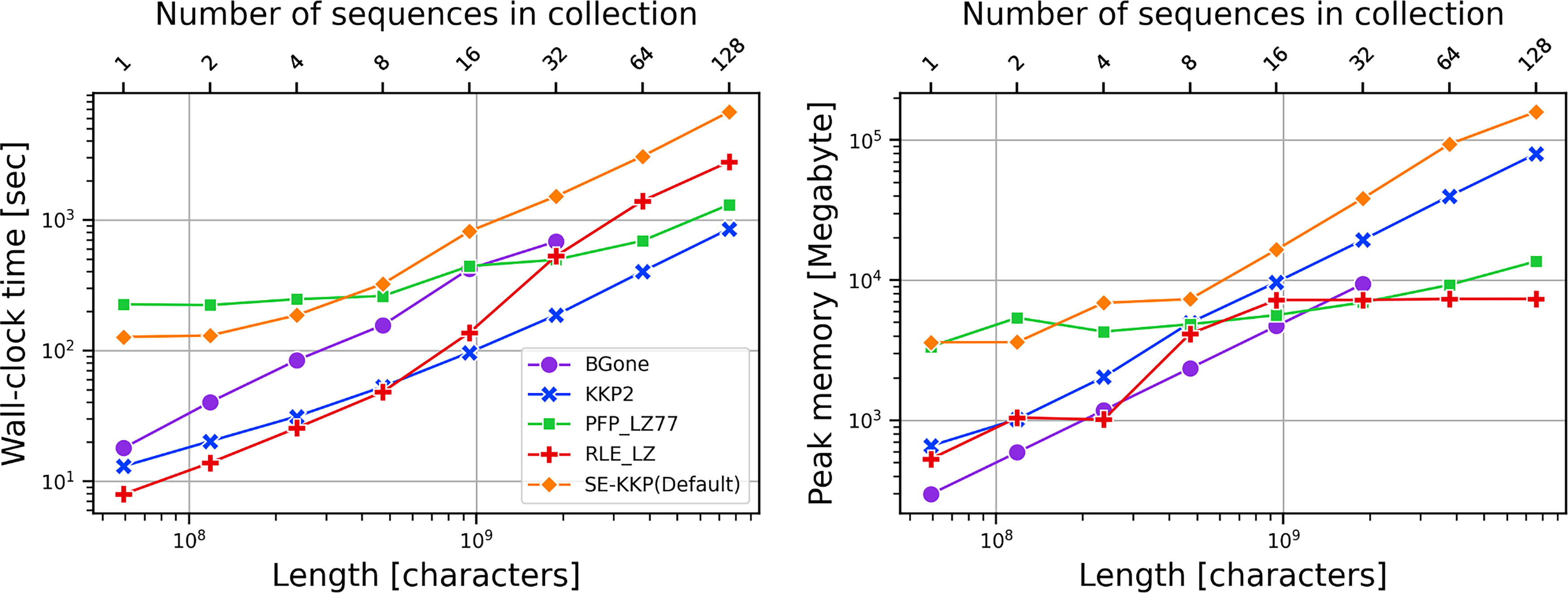
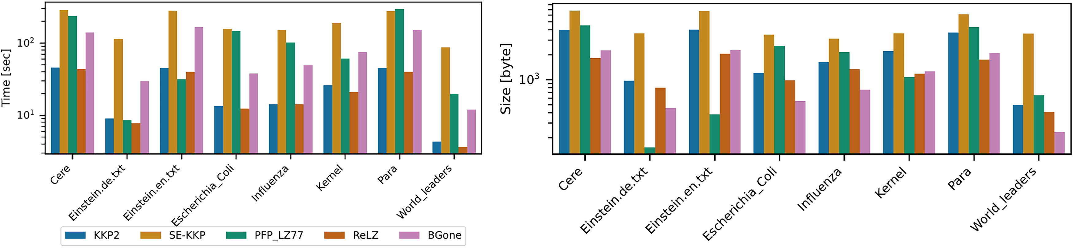
All methods, except the RLE-LZ algorithm, required less than 5GB of memory and were completed in less than 20 minutes. Figure 1 illustrates the memory (in bytes) and time (in seconds) of all methods. The SE-KKP algorithm used more time and memory than all other algorithms. Since SE-KKP is semi-external memory, it used a substantial amount of hard disk for each experiment. In particular, SE-KKP consumed between 2.47GB and 36.51GB of hard disk space across different datasets. The PFP-LZ77 required the least memory and time out of all methods on the Einstein.de.txt, Einstein.en.txt datasets, as these two datasets have a higher repetitiveness. The performance of the BGone algorithm is comparable to that of PFP-LZ77.
Time and memory required by all algorithms for the Pizza&Chili dataset. The left graph shows the time required to build the LZ77 factors. The graph on the right shows the memory required to compute the LZ77.
Results on Salmonella
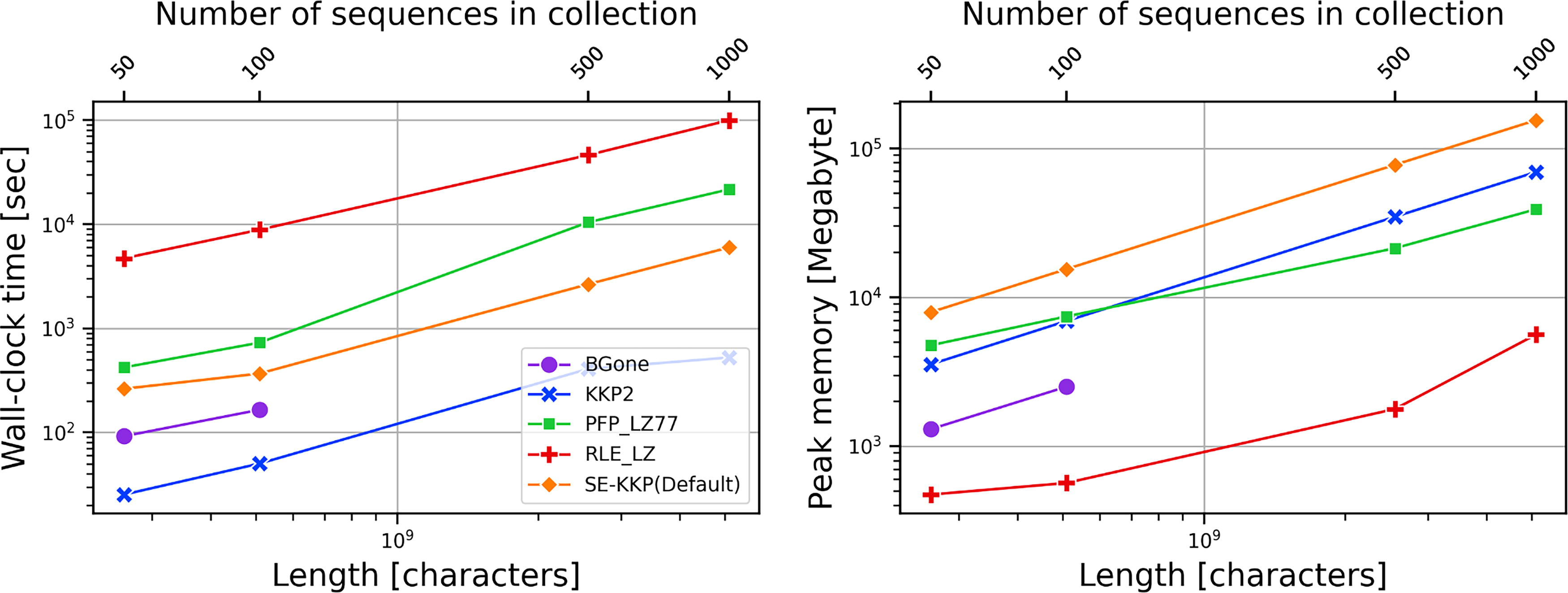
In this experiment, we set a time limit of 24 hours. However, the RLE-LZ algorithm was unable to complete the experiment within this limit. To evaluate its performance more precisely, we extended the time limit and observed that it required 27 hours to process the data set with 1,000 copies of Salmonella. Although RLE-LZ consumed the least memory, it required the most time across all datasets. The SE-KKP algorithm consistently used the most memory and required 19.71 GB, 38.78 GB, 211.03 GB, and 428.60 GB of hard disk space in various scenarios. KKP2 was the fastest in this experiment, and its memory usage was similar to that of PFP-LZ77. However, our analysis indicates that KKP2’s memory consumption increases at a faster rate than the PFP-LZ77 method when processing larger datasets. The BGone algorithm could only complete processing 100 copies of the Salmonella dataset, as its memory requirements exceeded our available 128 GB RAM when attempting to process larger datasets. In the experiments it could complete, BGone demonstrated the second-lowest memory consumption and the second-fastest execution time, indicating its suitability for smaller datasets. Results shown in Figure 2.
Time and memory required by all the algorithms on the Salmonella dataset. The left graph shows the time required to build the LZ77 factors. The graph on the right shows the memory required to compute the LZ77.
Results on chromosome 19
In this experiment, we set a time limit of 24 hours. The BGone algorithm could only process data sets smaller than 64 copies of chromosome 19. For datasets with fewer than 16 copies, BGone uses the least memory and is only slower than the RLE-LZ and KKP2 algorithms. Although other algorithms showed increasing resource requirements as the size of the dataset increased, the PFP-LZ77 method demonstrated a more stable performance trend. As the size of the data set increased, SE-KKP consistently showed the poorest performance, becoming the slowest and most memory-intensive. Specifically, when the data set is larger than 16 copies, SE-KKP is 7.63 to 8.45 times slower than the KKP2 algorithm and requires 2.92 to 11.64 times more RAM than PFP-LZ77. As shown in Figure 3, the PFP-LZ77 method demonstrated the most stable performance in both time and space on varying dataset sizes. This stability indicates that, for large datasets, PFP-LZ77 provides a more reliable approach to construct the 77 factors.
Time and Memory required by all the algorithms on the Chromosome 19 dataset. The left graph shows the time required to build the LZ77 factors. The graph on the right shows the memory required to compute the LZ77.
Recommendations
Based on our experimental evaluation, we recommend KKP2 and PFP-LZ77 as balanced and reliable choices to compress large-scale genomic data, offering strong performance in both runtime and memory usage across a variety of datasets. These algorithms consistently performed well on highly repetitive sequences, such as those in the Pizza&Chili corpus, as well as on real-world genomic data, including Salmonella genomes. KKP2, in particular, was notable for its speed, while PFP-LZ77 offers additional flexibility through its use of PFP and support for CST queries. RLE-LZ, although the most memory-efficient algorithm tested, demonstrated significantly longer runtimes and did not complete on the largest datasets, making it suitable only in highly memory-constrained environments where execution time is not a concern. SE-KKP proved effective in external memory settings, making it an appropriate option for datasets that exceed main memory limits, though it comes with increased resource usage. In practice, the availability of robust, well-documented, and actively maintained implementations, such as those for KKP2 and PFP-LZ77, should be a key consideration when selecting a compression strategy, as this can significantly affect integration and long-term usability. Although algorithms like KKP3 and BGone employ lazy evaluation techniques, our results do not indicate substantial runtime advantages of this design, particularly compared to alternatives such as KKP2. Ultimately, no single algorithm dominates in all scenarios; therefore, researchers and practitioners should carefully consider the trade-offs between time, space, and implementation maturity when selecting an algorithm based on 77 for genomic data compression.
CONCLUSION AND FUTURE WORK
Throughout this review, we have thoroughly explored the evolution and enhancement of the 77 algorithm and its derivatives, particularly focusing on their applications in genomic data compression. The continuous growth of genomic data requires efficient compression solutions that can effectively manage and utilize these vast datasets. Traditional 77 algorithms, while fundamental in the realm of lossless data compression, require significant adaptations to meet the unique demands of genomic sequences characterized by their repetitive nature. The advancements discussed in this article highlight significant strides in algorithmic innovation aimed at optimizing 77 for better handling of large-scale genomic data. We have examined a variety of specialized algorithms that not only improve compression ratios but also enhance processing efficiencies in both software and hardware implementations. These adaptations make it feasible to manage, store, and analyze genomic data more effectively, supporting the broader goals of genomic research and clinical applications.
Moreover, the integration of LZ77-based algorithms into hardware platforms represents a promising avenue for overcoming the throughput limitations of software-based compression. This approach can potentially unlock real-time processing capabilities, essential for applications requiring immediate data analysis, such as the compression of pangenomic datasets. In the future, the ongoing development of LZ77-based compression technologies will undoubtedly play a critical role in the bioinformatics field. Continued innovations are expected to further refine these algorithms, making them more adaptable to the evolving landscape of genomic data. Furthermore, exploring synergies between algorithmic improvements and hardware accelerations will be crucial to achieving the scalability and efficiency required for future applications in biological data compression, software distribution, streaming media, and medical imaging data. In the following, we highlight some specific areas that warrant future research.
Merging 77 factorizations
There are many large sequence datasets that grow rapidly, such as GenomeTrakr (Timme et al., 2019) and MetaSub (Mason et al., 2016), which update frequently. Currently, when applying 77 factorization to these datasets, we need to regenerate the 77 factorization each time the datasets are updated. This process is time-consuming and computationally expensive. However, if we can update the 77 factors generated from previous versions of the dataset, it would save a significant amount of time and computational resources. As described by Oliva et al. (2021) and Muggli et al. (2019), dynamic data structures and algorithms for merging BWTs have been successfully applied to address similar challenges in other contexts. These techniques could be adapted to the 77 construction process.
External memory construction
Although there have been several methods that use external memory for 77 factorization—as discussed in Subsection 3.10—this area still deserves continued attention since data sets continue to grow substantially larger and will surpass main memory. Current algorithms that rely on external memory require substantially more time than existing methods, which is unsurprising given the gap between the time required to access main memory and access to the hard disk. However, there are still opportunities for advancement in this area. For instance, consider the PFP-LZ77 algorithm. Previously, the PFP parsing for the input string S was computed in a single step within main memory. However, this process can be adapted to handle larger data sets by dividing the input string into manageable blocks that fit into main memory. Each block can then be processed independently using the PFP-LZ77 algorithm to produce partial 77 factorizations. After processing all blocks, a merging phase can combine these partial factorizations into a global factorization. Multithreading can be applied to this process, significantly speeding up the processing time. Furthermore, using disk-based data structures, such as B-trees, can facilitate the efficient search operations required by the 77 algorithm, enhancing the algorithm’s performance in an external memory context.
GPU implementation
Exploring the implementation of 77 on GPU is a promising direction for future research. GPUs are well-suited for parallel processing tasks due to their ability to handle many computations simultaneously. Although some existing research has successfully applied GPUs to fundamental data structures such as suffix arrays (Büren et al., 2019), more complex algorithms such as 77 have not been extensively explored. A key challenge in implementing 77 on GPUs is efficiently partitioning input data and managing memory to ensure that each GPU thread operates independently. One approach is to divide the input string into smaller blocks that fit into GPU memory and process each block in parallel. After processing, the partial 77 factorizations can be merged into a global factorization. Minimizing data transfer between the CPU and the GPU and using asynchronous transfers can further enhance performance. Future research could focus on optimizing these parallel algorithms, exploring hybrid CPU-GPU approaches, and testing the implementation on real-world datasets to validate its effectiveness.
Footnotes
DATA AVAILABILITY STATEMENT
We used the real-world datasets from the Pizza&Chili repetitive corpus, Salmonella genomes obtained from the NCBI website. The Pizza&Chili repetitive corpus consists of repetitive texts that vary in length and alphabet size, providing a diverse set of inputs to test the performance of the algorithms. This data set is widely used for benchmarking as it includes standard test cases that have been extensively studied in previous work on compression. This data set can be accessed at https://pizzachili.dcc.uchile.cl/biblio.html. For Salmonella data sets, we used four sets that contain 50, 100, 500, and 1,000 copies of the Salmonella genome sequence. All Salmonella genome sequences are available at https://www.ncbi.nlm.nih.gov/datasets/genome/?taxon=590. For human chromosome 19 analysis, we constructed eight datasets containing 1, 2, 4, 8, 16, 32, 64, and 128 copies of the chromosome 19 genome sequence. All chromosome 19 sequences were accessed through the NCBI gene database https://www.ncbi.nlm.nih.gov/gene?Db=gene&Cmd=DetailsSearch&Term=148223.
AUTHORS’ CONTRIBUTIONS
A.H.: Theoretical and formal analysis, data curation, writing—original draft, writing—review and editing, experiments. C.B.: Funding acquisition, supervision, writing—original draft, writing—review and editing, reviewing experiments and analysis.
AUTHOR DISCLOSURE STATEMENT
The authors have no conflict of interest.
FUNDING INFORMATION
This research was funded by NSF:SCH:INT (Grant No. 2013998) and NIH/NHGRI (Grant No. R01HG011392).
References
1.
BingmannT, FischerJ, OsipovV, et al.Inducing Suffix and LCP Arrays in External Memory. ACM J Exp Algorithmics, 2016; 21:1–27.
2.
BoucherC, et al.PFP Compressed Suffix Trees. In: Proceedings of the SIAM Symposium on Algorithm Engineering and Experiments (ALENEX). 2021; pp. 60–72.
3.
BürenF, et al.Suffix Array Construction on Multi-GPU Systems. In: Proceedings of the 28th International Symposium on High-Performance Parallel and Distributed Computing. 2019; pp. 183–194.
4.
BurrowsM, WheelerDJ. A Block-Sorting Lossless Data Compression Algorithm. Technical Report 0769518966, Digital Equipment Corporation; 1994.
5.
CastelliR, et al.Lossless compression of nanopore sequencing raw signals. In: Proceedings of the Bioinformatics and Biomedical Engineering (IWBBIO). Springer Nature; 2024; pp. 130–141.
6.
CrochemoreM, IlieL. Computing longest previous factor in linear time and applications. Information Processing Letters, 2008; 106(2):75–80.
7.
DementievR, et al.STXXL: Standard template library for XXL data sets. In: Proceedings of the 13th Annual European Conference on Algorithms. Springer-Verlag; 2005; pp. 640–651.
8.
EllertJ. Sublinear Time Lempel-Ziv (LZ77) Factorization. In: Proceedings of the 30th International Symposium String Processing and Information Retrieval (SPIRE). 2023; pp. 171–187.
9.
FerraginaP, ManziniG. Opportunistic data structures with applications. In: Proceedings of the 41st Annual Symposium on Foundations of Computer Science (FOCS). 2000; pp. 390–398.
GotoK, BannaiH. Simpler and faster Lempel Ziv factorization. In: Proceedings of the IEEE Data Compression Conference (DCC). 2013; pp.133–142.
12.
GotoK, BannaiH. Space Efficient Linear Time Lempel-Ziv Factorization for Small Alphabets. In: Data Compression Conference (DCC), 2014; pp. 163–172.
13.
GrossiR, VitterJ. Compressed suffix arrays and suffix trees with applications to text indexing and string matching. SIAM J Comput, 2005; 35(2):378–407.
14.
HongA, et al.LZ77 via Prefix-Free Parsing. In: Proceedings of the Symposium on Algorithm Engineering and Experiments (ALENEX). 2023; pp. 123–134.
15.
KärkkäinenJ, et al.Lightweight Lempel-Ziv Parsing. In: Proceedings of the 12th International Symposium on Experimental Algorithms (SEA). 2013b; pp. 139–150.
16.
KärkkäinenJ, et al.Linear Time Lempel-Ziv Factorization: Simple, Fast, Small. In: Proceedings of the 24th Annual Symposium on Combinatorial Pattern Matching (CPM). 2013a; pp. 189–200.
17.
KärkkäinenJ, et al.Permuted longest-common-prefix array. In: Proceedings of the 20th Annual Symposium on Combinatorial Pattern Matching. 2009; pp. 181–192.
18.
KärkkäinenJ, KempaD. Engineering a lightweight external memory suffix array construction algorithm. MathComputSci, 2017; 11(2):137–149.
19.
KärkkäinenJ, KempaD, PuglisiSJ. Lempel-Ziv Parsing in External Memory. In: Proceedings of the IEEE Data Compression Conference (DCC). 2014; pp. 153–162.
20.
KarpRM, RabinMO. Efficient randomized pattern-matching algorithms. IBM J Res & Dev, 1987; 31(2):249–260.
21.
KasaiT, et al.Linear-time longest-common-prefix computation in suffix arrays and its applications. In: Proceedings of the 18th Annual Symposium on Combinatorial Pattern Matching (CPM), Volume 2089. 2001; pp. 181–192.
22.
KempaD, KociumakaT. Lempel-Ziv (LZ77) factorization in sublinear time. In: Proceedings of the 65th Annual Symposium on Foundations of Computer Science (FOCS). IEEE; 2024; pp. 2045–2055.
23.
KempaD, PuglisiSJ. Lempel-Ziv Factorization: Simple, Fast, Practical. In: Proceedings of the SIAM Symposium on Algorithm Engineering and Experiments (ALENEX). 2013; pp. 103–112.
LiuWJ, NongG, ChanWh, et al.Improving a lightweight 77 computation algorithm for running faster. Softw Pract Exper, 2016; 46(9):1201–1217.
26.
LukensLN, QuijadaPA, UdallJ, et al.Genome redundancy and plasticity within ancient and recent Brassica crop species. Biological Journal of the Linnean Society, 2004; 82(4):665–674.
ManberU, MyersGW. Suffix arrays: A new method for on-line string searches. SIAM J Comput, 1993; 22(5):935–948.
29.
MasonC, et al.The metagenomics and metadesign of the subways and urban Biomes (MetaSUB) international consortium inaugural meeting report. Microbiome, 2016; 4(1):24.
30.
MölderF, JablonskiKP, LetcherB, et al.Sustainable data analysis with Snakemake. F1000Res, 2021; 10:33.
31.
MuggliMD, AlipanahiB, BoucherC. Building large updatable colored de Bruijn graphs via merging. Bioinformatics, 2019; 35(14):i51–i60; doi: 10.1093/bioinformatics/btz350
32.
NongG. Practical linear-time O(1)-workspace suffix sorting for constant alphabets. ACM Trans Inf Syst, 2013; 31(3):1–15.
33.
NorriT, CazauxB, DöngesS, et al.Founder reconstruction enables scalable and seamless pangenomic analysis. Bioinformatics, 2021; 37(24):4611–4619.
34.
OhlebuschE, GogS. Lempel-Ziv factorization revisited. In: Proceedings of the 22nd Annual Symposium on Combinatorial Pattern Matching (CPM). 2011; pp. 15–26.
35.
OlivaM, et al.Efficiently Merging r-indexes. In: Proceedings of the IEEE Data Compression Conference (DCC). 2021; pp. 203–212; doi: 10.1109/DCC50243.2021.00028
The 1000 Genomes Project Consortium. A global reference for human genetic variation. Nature, 2015; 526(7571):68–74.
40.
TimmeRE, et al.Utilizing the public GenomeTrakr database for foodborne pathogen traceback. Foodborne Bacterial Pathogens: methods and Protocols, 2019 pages:201–212.
41.
WertenbroekR, RubinacciS, XenariosI, et al.XSI—a genotype compression tool for compressive genomics in large biobanks. Bioinformatics, 2022; 38(15):3778–3784.
42.
ZivJ, LempelA. A universal algorithm for sequential data compression. IEEE Trans Inform Theory, 1977; 23(3):337–343.