Enhanced Accuracy of Continuous Glucose Monitoring by Online Extended Kalman Filtering

Abstract

Background:

Most continuous glucose monitoring (CGM) devices measure a current, proportional to the interstitial glucose (IG) concentration, which is converted into a glucose level by a standard device calibration step that exploits some blood glucose (BG) references. However, data show that deterioration of sensor gain may occur, which can affect CGM output by a systematic and possibly large (e.g., up to 15/20 mg/dL) error. Enhanced calibration algorithms for improving the accuracy of CGM are thus of critical importance, especially in real-time applications.

Methods:

In this work we present an enhanced Bayesian calibration method that can be implemented online by using the Extended Kalman Filter. The method takes into account the existence of BG-to-IG kinetics by incorporating a population convolution model and exploits only four BG reference samples per day.

Results:

The new method is successfully applied on 10 simulated virtual patients. Its performance in improving the accuracy of CGM profiles is significantly better than that of other current calibration procedures. Furthermore, the new method is shown to be robust to changes in its parameters. Improvement in the accuracy of CGM is also shown on a representative subject.

Conclusions:

Realistic simulations show that the new enhanced calibration method significantly improves the accuracy of CGM signals, suggesting potential benefits by its inclusion in real-time applications of CGM devices.

Introduction

C ontinuous glucose monitoring (CGM) devices can measure, in real-time, the glycemic level at a continuous time for up to several days,^1,2 allowing the improvement of diabetes management.^3
–5 Most commercial CGM systems, e.g., the Seven^® (DexCom, Inc., San Diego, CA),⁶ the FreeStyle Navigator^® (Abbott Diabetes Care, Alameda, CA),⁷ and the CGMS^® (Medtronic Minimed, Inc., Northridge, CA),⁸ exploit the glucose oxidase principle, which requires that the current levels (measured, e.g., in mA) be transformed into glucose levels (given, e.g., in mg/dL) by exploiting a transformation rule with parameters determined using one or more glucose reference, e.g., self-monitoring of blood glucose (SMBG), samples. This step is commonly referred to as standard device calibration.

In order to reduce invasiveness, CGM sensors are placed in the subcutis and thus measure interstitial glucose (IG) rather than blood glucose (BG) concentration. In dynamic conditions, IG and BG differ because of the existence of BG-to-IG kinetics. To show this, Figure 1 displays a comparison, performed in a clinical study,⁹ between BG reference samples (stars), collected every 15 min (measured with a YSI BG analyzer [YSI, Inc., Yellow Springs, OH]), and a CGM profile (line), collected using a subcutaneous sensor (FreeStyle Navigator); amplitude and phase distortions are evident. The BG-to-IG kinetics have been described by a two-compartment model (Fig. 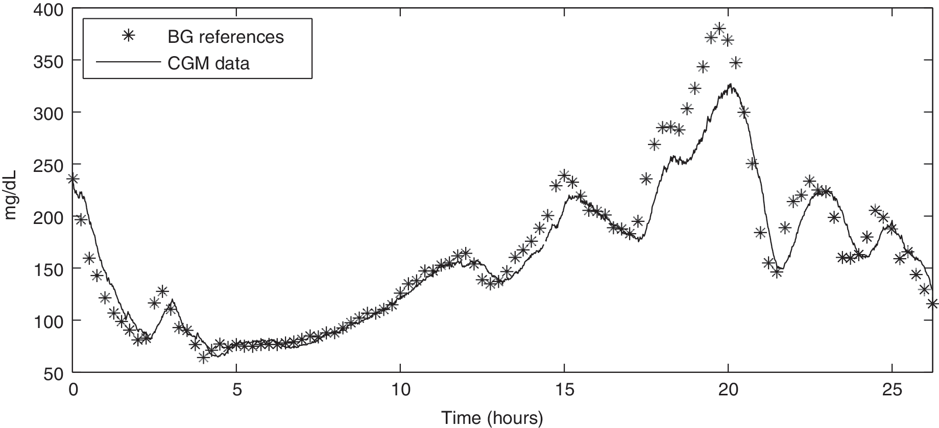2),¹⁰ from which one can easily obtain: \documentclass{aastex} \usepackage{amsbsy} \usepackage{amsfonts} \usepackage{amssymb} \usepackage{bm} \usepackage{mathrsfs} \usepackage{pifont} \usepackage{stmaryrd} \usepackage{textcomp} \usepackage{portland, xspace} \usepackage{amsmath, amsxtra} \pagestyle{empty} \DeclareMathSizes {10} {9} {7} {6} \begin{document} \begin{align*} {\rm I}\dot{{\rm G}}(t) = - \frac {1} {\tau} {\rm IG } (t) + \frac {g} {\tau} {\rm BG} (t) \tag { 1 } \end{align*} \end{document}

FIG. 1.

Representative real data taken from Kovatchev et al.⁹: BG reference samples (stars) versus CGM data (line) profiles.

FIG. 2.

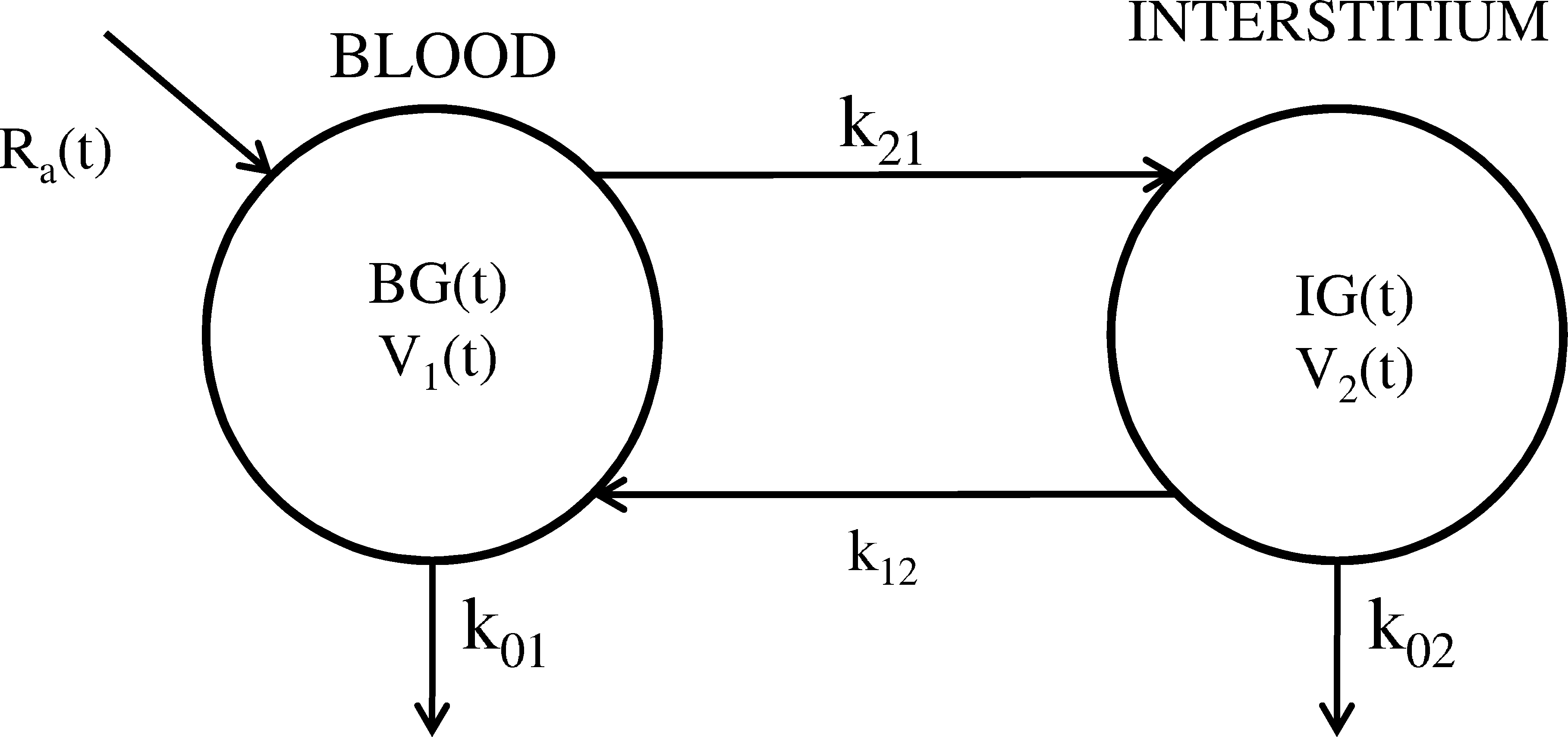
Two-compartment model describing the BG-to-IG kinetics. In order to obtain the formulation of Eq. 1, the following reparameterization has been used: g = (k ₂₁ V ₁/V ₂)τ and τ = 1/(k ₀₂ + k ₁₂).

In other terms, IG can be interpreted as the output of a first-order linear system driven by BG, where g represents the “static gain” of the “BG-to-IG system,” which we can consider equal to 1,¹¹ and τ is the time constant of the system, which could vary between individuals. The system acts as a low-pass filter and introduces a distortion (attenuation in amplitude and distortion in phase) that is well observable, e.g., in time window 0–5 h of Figure 1. The existence of BG-to-IG kinetics, however, is not able to explain some discrepancies that are evident along the y-axis, e.g., in the interval 12–22 h. This difference seems due to a change of behavior of the CGM sensor performance after the initial standard device calibration.

The fact that CGM profiles may differ from BG profiles because of calibration problems can be critical in several applications, e.g., artificial pancreas methods relying on CGM output.^12,13 Improving the accuracy of CGM data is therefore an important task to deal with in real-time. In this work we present a new enhanced calibration method that can potentially work in cascade to standard calibration of any CGM device. The aim of this enhanced calibration is to process the sensor outcome in order to improve the quality of the CGM readings. The method is based on the Extended Kalman Filter (EKF), which, by taking into account the BG-to-IG kinetics, four SMBG samples per day, and a model of the time–behavior of sensor accuracy, significantly enhances the quality of CGM data in real-time applications. The new method is successfully validated on a simulated dataset reproducing 10 virtual patients. In particular, the method is shown superior in terms of both root mean square error (RMSE) and robustness with respect to other current calibration procedures proposed in the literature. In addition, a representative subject dataset is also used show the practical usability of the method.

CGM Calibration: State of the Art

Different calibration procedures have been presented in the literature. A preliminary and important work that considered the efficiency of calibration was performed by the DirecNet Study Group,¹⁴ which retrospectively analyzed the improvement in CGMS sensor accuracy by modifying the number and timing of the calibration points. Results showed that the timing of the calibration points is even more important than the number. In particular, performing calibrations during periods of relative glucose stability, i.e., where the point-to-point difference due to the BG-to-IG kinetics is minimized, significantly improves the accuracy.

The most adopted calibration strategy^15,16 is the one presented by King et al.,¹⁷ which is based on the linear regression model of Eq. 2: \documentclass{aastex} \usepackage{amsbsy} \usepackage{amsfonts} \usepackage{amssymb} \usepackage{bm} \usepackage{mathrsfs} \usepackage{pifont} \usepackage{stmaryrd} \usepackage{textcomp} \usepackage{portland, xspace} \usepackage{amsmath, amsxtra} \pagestyle{empty} \DeclareMathSizes {10} {9} {7} {6} \begin{document} \begin{align*} y = ax + b \tag{2} \end{align*} \end{document}

where a and b are calibration parameters that are determined by fitting them against a couple of BG (y) and CGM (x) pairs collected at the same time.^17,18 The procedure works retrospectively and exploits all available BG references. This method suffers by several limitations. First, it can be applied only retrospectively. Second, it does not take into account the distortion introduced by the BG-to-IG kinetics. For instance, it does not consider that, when glucose is changing rapidly, e.g., after a meal, BG and IG are significantly different (e.g., BG can be 20 mg/dL higher than IG). Finally, it cannot deal with a possible time-varying behavior of sensor performance (i.e., the parameters of Eq. 2 are estimated only once for the entire monitoring).

Another approach is presented in the work of Kuure-Kinsey et al.,¹⁹ where a dual-rate Kalman filter is presented to improve the accuracy of CGM data. The procedure exploits sparse SMBG measurements and estimates in real-time the sensor gain. However, this algorithm also does not account for BG-to-IG kinetics.

A comprehensive description of the CGM measurement process is due to Knobbe and Buckingham.¹¹ In their work, the BG-to-IG kinetics model was explicitly taken into account in order to reconstruct BG levels at continuous time from CGM measurements. In such an attempt, a state-space Bayesian framework exploiting a priori knowledge of the unknown variables was adopted (for details see The state space model), and an EKF was implemented to perform state estimation. However, in the article of Knobbe and Buckingham¹¹ the EKF was tested on four subjects principally to estimate the BG concentration. The calibration of CGM was only a by-product of the method. Even if results were insightful, the robustness of the method was not fully assessed because validation on simulated data was missing.

Below we start from the work of Knobbe and Buckingham¹¹ and further develop the approach in order to tackle calibration issues. In particular, our method aims to improve the accuracy of CGM data by performing an enhanced calibration, which works in cascade to the standard device calibration. Also, we design and implement a simulation strategy that is able to precisely define the domain of validity of the method.

Simulated Database

The database used for the validation of the method consists of 10 simulated type 1 diabetes virtual patients. Each subject file contains a 7-day simulated CGM profile and four simulated SMBG samples per day, created as described below.

First, BG profiles were created at 1-min time sampling by using an in silico type 1 diabetes simulator. Model parameters of the 10 virtual patients were randomly chosen from realistic distributions.^13,20,21 In this way, each 7-day BG time series has its own characteristics and differs from all the others. More specifically, to build the BG time-series, three meals per day were considered. In order to simulate real-life episodes, breakfast, lunch, and dinner times were allocated randomly within the following time intervals: 6:00–8:00 h for breakfast, 12:00–14:00 h for lunch, and 19:00–21:00 h for dinner. Carbohydrate intakes were differentiated from meal to meal and from day to day. Their quantities were drawn randomly from three different normal distributions with mean ± SD given by 45 ± 10 g (breakfast), 75 ± 10 g (lunch), and 85 ± 10 g (dinner).²⁰ For instance, Figure 3 displays the BG profile (black thick line) obtained for a representative subject (subject number 3) in a representative day (Day 6). SMBG samples were simulated by taking four BG samples per day and adding a measurement error with coefficient of variation (CV) of 2% (gray circles in Fig. 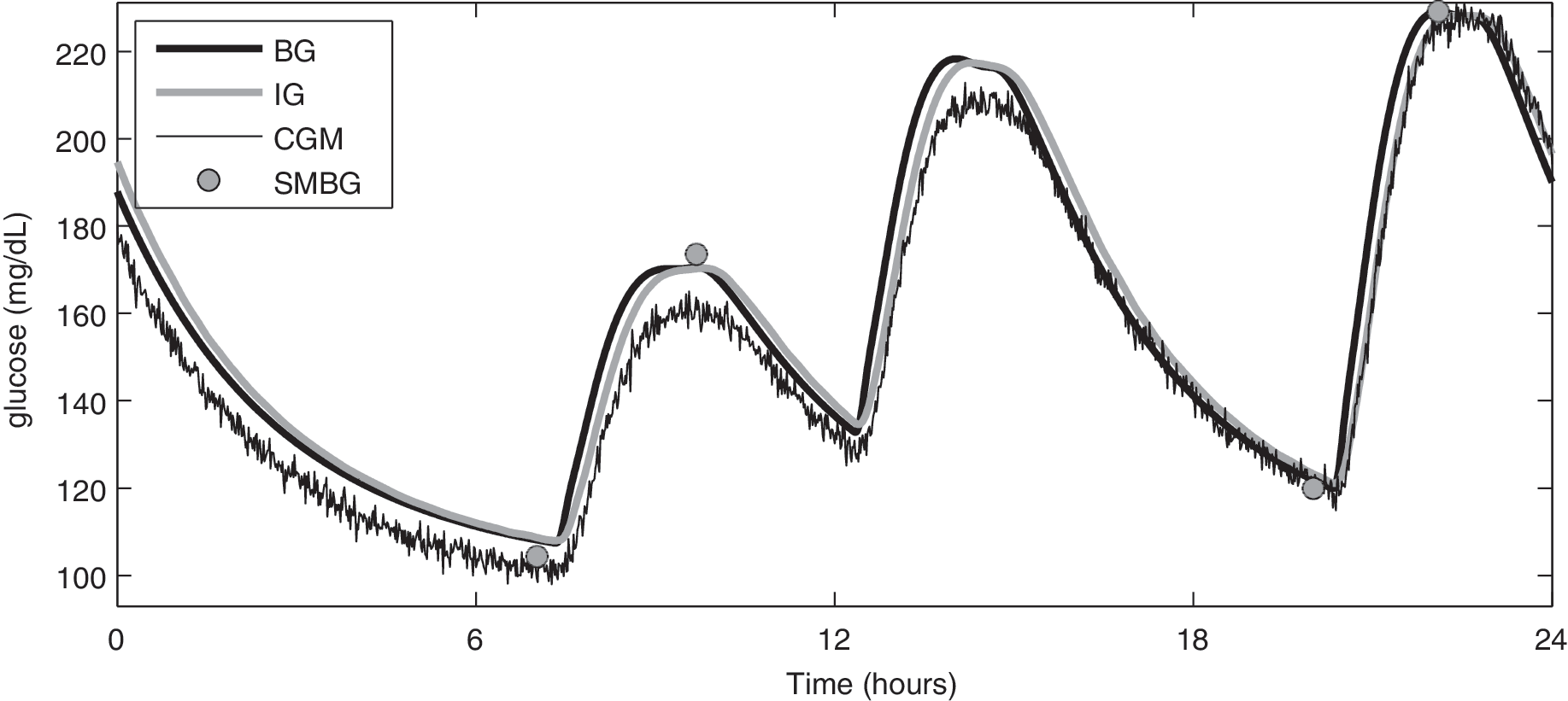3), as follows: \documentclass{aastex} \usepackage{amsbsy} \usepackage{amsfonts} \usepackage{amssymb} \usepackage{bm} \usepackage{mathrsfs} \usepackage{pifont} \usepackage{stmaryrd} \usepackage{textcomp} \usepackage{portland, xspace} \usepackage{amsmath, amsxtra} \pagestyle{empty} \DeclareMathSizes {10} {9} {7} {6} \begin{document} \begin{align*}{\rm SMBG} (k) = \varphi (k) {\rm BG} (k) + v_2 (k) \tag{3} \end{align*} \end{document}

FIG. 3.

Representative simulated virtual patient number 3, Day 6: actual BG (black thick line) and IG (gray thick line), measured CGM (black line), affected by random multiplicative calibration error (Eq. 5) and by random additive error (Eq. 4), and measured SMBG (gray circles), affected by additive noise (Eq. 3).

where φ(k) is a flag that is equal to 1 only when the SMBG sample is collected.

Then, by applying Eq. 1 with time-invariant parameters (i.e., g = 1 and τ = 12 min), IG concentrations are obtained (gray thick line in Fig. 3). Finally, the measured CGM profile (black thin line in Fig. 3) is obtained as: \documentclass{aastex} \usepackage{amsbsy} \usepackage{amsfonts} \usepackage{amssymb} \usepackage{bm} \usepackage{mathrsfs} \usepackage{pifont} \usepackage{stmaryrd} \usepackage{textcomp} \usepackage{portland, xspace} \usepackage{amsmath, amsxtra} \pagestyle{empty} \DeclareMathSizes {10} {9} {7} {6} \begin{document} \begin{align*}{\rm CGM} (k) = ( 1 + \alpha (k)) {\rm IG} (k) + v_1 (k)\tag{4} \end{align*} \end{document}

where IG(k) represents the interstitial glucose level at sample k, α(k) is a random multiplicative value that simulates the possibly time-varying deviation of the sensor gain from unitary level, and v ₁(k) is the random additive measurement error. In particular, v ₁(k) is modeled as a zero mean white Gaussian process with variance σ ² = 4 mg²/dL².^19,22,23 Here, the gain deviation α(k), which, from a theoretical point, resembles the scale factor of Knobbe and Buckingham,¹¹ is created as the triple integration of a zero mean white noise process w ₁(k): \documentclass{aastex} \usepackage{amsbsy} \usepackage{amsfonts} \usepackage{amssymb} \usepackage{bm} \usepackage{mathrsfs} \usepackage{pifont} \usepackage{stmaryrd} \usepackage{textcomp} \usepackage{portland, xspace} \usepackage{amsmath, amsxtra} \pagestyle{empty} \DeclareMathSizes {10} {9} {7} {6} \begin{document} \begin{align*} \alpha ( k + 1 ) = 3 \alpha (k) - 3 \alpha (k - 1) + \alpha ( k - 2) + w_1 (k) \tag{5} \end{align*} \end{document}

In the literature no models for simulating/generating the gain deviation α(k) have been proposed. Here, we decided to propose it as in Eq. 5 by using three, rather than one or two, integrators because this better simulates the experienced loss of performance of CGM sensors during long-term monitoring. An example of α(k) profile is reported in the bottom panel of Figure 4 (gray dashed line), where calibration errors of the order of 10% of the reference value are obtained. Of note is that the model for α(k) is zero mean. As in the work of Knobbe and Buckingham,¹¹ this assumption can be taken without any loss of generality because the introduction of a bias term would not introduce any change in the performance of the method.

FIG. 4.

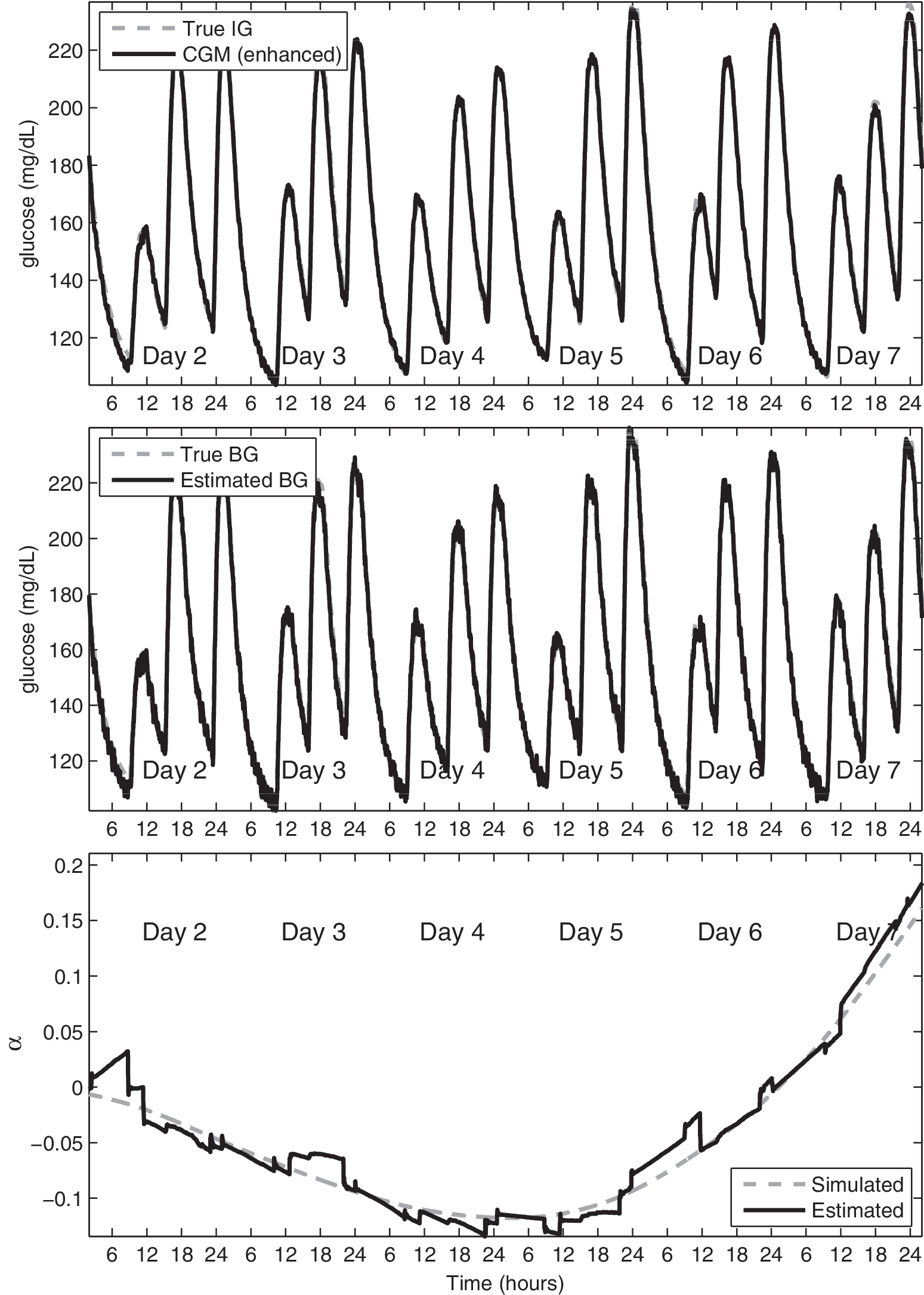
Representative subject number 3. (Top) True IG (gray dashed) versus enhanced CGM (black) time series. (Middle) True (gray dashed) versus estimated (black) BG concentrations. (Bottom) Simulated (gray dashed) versus estimated (black) α profiles.

Enhanced Bayesian Calibration Method (BCM)

The new online calibration method exploits a stochastic framework and Bayesian estimator. For sake of simplicity, in the following, the acronym BCM will be used. As detailed below, the inputs of BCM are the noisy CGM time series (black thin line in Fig. 3) and the four SMBG samples per day (gray circles in Fig. 3). The outputs are the enhanced CGM time series, i.e., an estimation of the IG profile, an estimation of the BG concentration, and, as a by-product, an estimation of the gain deviation α(k).

BCM exploits a state space model representation of all unknown signals (see The state space model below), and it is implemented by using EKF (see The EKF implementation below).

The state space model

Assuming that measured CGM and BG are described as in Eqs. 3 and 4, the next step is to choose suitable a priori models for the unknown signals BG, IG, and α on the considered 1-min evenly spaced grid. The model selected to describe the unknown BG at 1-min time sampling is an integrated random walk model: \documentclass{aastex} \usepackage{amsbsy} \usepackage{amsfonts} \usepackage{amssymb} \usepackage{bm} \usepackage{mathrsfs} \usepackage{pifont} \usepackage{stmaryrd} \usepackage{textcomp} \usepackage{portland, xspace} \usepackage{amsmath, amsxtra} \pagestyle{empty} \DeclareMathSizes {10} {9} {7} {6} \begin{document} \begin{align*}{\rm BG} (k + 1) = 2{\rm BG} (k) - {\rm BG} (k - 1) + w_2 (k) \tag{6} \end{align*} \end{document}

where BG(k) represents the blood glucose value at the k-th sample and w ₂(k) is a zero mean Gaussian noise with variance equal to \documentclass{aastex} \usepackage{amsbsy} \usepackage{amsfonts} \usepackage{amssymb} \usepackage{bm} \usepackage{mathrsfs} \usepackage{pifont} \usepackage{stmaryrd} \usepackage{textcomp} \usepackage{portland, xspace} \usepackage{amsmath, amsxtra} \pagestyle{empty} \DeclareMathSizes {10} {9} {7} {6} \begin{document} \begin{align*} \lambda_2^2 \end{align*} \end{document} . The multiple integration of a white noise process is commonly used in Bayesian signal estimation to represent a regular signal, e.g., a physiological process.²⁴ In addition, this particular model has also been recently used to represent the regular pattern of the glycemic signal in a context of CGM data denoising.²⁵ Here, the choice of two, rather than one or three, integrators has been performed by a preliminary analysis on real, high-frequently sampled, BG datasets taken from the literature.²⁶

The a priori model for IG simply reflects the continuous-time differential equation of Eq. 1, which, after discretization, turns into Eq. 6: \documentclass{aastex} \usepackage{amsbsy} \usepackage{amsfonts} \usepackage{amssymb} \usepackage{bm} \usepackage{mathrsfs} \usepackage{pifont} \usepackage{stmaryrd} \usepackage{textcomp} \usepackage{portland, xspace} \usepackage{amsmath, amsxtra} \pagestyle{empty} \DeclareMathSizes {10} {9} {7} {6} \begin{document} \begin{align*}{\rm IG} (k + 1) = \left(1 - \frac{1}{\tau} \right) {\rm IG} (k) + \frac {g} {\tau} {\rm BG} (k) \tag { 7 } \end{align*} \end{document}

Finally, the a priori model for α(k) is the triple integration of a zero mean white noise process w ₁(k) with variance equal to \documentclass{aastex} \usepackage{amsbsy} \usepackage{amsfonts} \usepackage{amssymb} \usepackage{bm} \usepackage{mathrsfs} \usepackage{pifont} \usepackage{stmaryrd} \usepackage{textcomp} \usepackage{portland, xspace} \usepackage{amsmath, amsxtra} \pagestyle{empty} \DeclareMathSizes {10} {9} {7} {6} \begin{document} \begin{align*} \lambda_1^2 \end{align*} \end{document} (see Eq. 5).

In order to obtain a state-space dynamic model, formulated by letting x ₁(k) = BG(k), x ₂(k) = BG(k − 1), x ₃(k) = IG(k), x ₄(k) = α(k), x ₅(k) = α(k − 1), and x ₆(k) = α(k − 2), one has: \documentclass{aastex} \usepackage{amsbsy} \usepackage{amsfonts} \usepackage{amssymb} \usepackage{bm} \usepackage{mathrsfs} \usepackage{pifont} \usepackage{stmaryrd} \usepackage{textcomp} \usepackage{portland, xspace} \usepackage{amsmath, amsxtra} \pagestyle{empty} \DeclareMathSizes {10} {9} {7} {6} \begin{document} \begin{align*}\left[ \begin{matrix}x_1 ( k + 1 ) \\ x_2 ( k + 1 ) \\ x_3 ( k + 1 ) \\ x_4 ( k + 1 ) \\ x_5 ( k + 1 ) \\ x_6 ( k + 1) \end{matrix} \right] = \left[ \begin{matrix}2x_1 ( k ) - x_2 ( k) \\ x_1 ( k ) \\ ( 1 - ( 1 / \tau ) x_3 ( k ) + ( 1 / \tau ) x_1( k ) \\ 3x_4 ( k ) - 3x_5 ( k ) + x_6 ( k ) \\ x_4 ( k ) \\ x_5 ( k ) \end{matrix} \right] + \left[ \begin{matrix}w_2 ( k ) \\ 0 \\ 0 \\ w_1 ( k ) \\ 0 \\ 0\end{matrix} \right] \tag{8}\end{align*} \end{document}

The measurements model, obtained from Eqs. 3 and 4, reads: \documentclass{aastex} \usepackage{amsbsy} \usepackage{amsfonts} \usepackage{amssymb} \usepackage{bm} \usepackage{mathrsfs} \usepackage{pifont} \usepackage{stmaryrd} \usepackage{textcomp} \usepackage{portland, xspace} \usepackage{amsmath, amsxtra} \pagestyle{empty} \DeclareMathSizes {10} {9} {7} {6} \begin{document} \begin{align*}\left[ \begin{matrix}y_1 ( k ) \\ y_2 ( k ) \end{matrix} \right] = \left[ \begin{matrix}x_3 ( k ) x_4 ( k ) \\ \varphi ( k ) x_1 ( k ) \end{matrix} \right] + \left[ \begin{matrix}v_1 ( k ) \\ v_2 ( k ) \end{matrix} \right] \tag{9}\end{align*} \end{document}

where y ₁(k) and y ₂(k) are the measured CGM and BG signals. In Eq. 9 a nonlinear relationship between the two states x ₃(k) and x ₄(k) [corresponding to IG(k) and α(k)] is present. For this reason, in order to recover the estimates \documentclass{aastex} \usepackage{amsbsy} \usepackage{amsfonts} \usepackage{amssymb} \usepackage{bm} \usepackage{mathrsfs} \usepackage{pifont} \usepackage{stmaryrd} \usepackage{textcomp} \usepackage{portland, xspace} \usepackage{amsmath, amsxtra} \pagestyle{empty} \DeclareMathSizes {10} {9} {7} {6} \begin{document} \begin{align*}{\hat x} (k) \end{align*} \end{document} starting from y ₁(k) and y ₂(k), the version of the Kalman filter for nonlinear problems, i.e., the so-called EKF, has to be used.

The EKF implementation

In general, an EKF^27,28 can be used to provide a minimum variance estimate of the state vector x of a dynamic discrete-time process governed by a nonlinear stochastic differential equation: \documentclass{aastex} \usepackage{amsbsy} \usepackage{amsfonts} \usepackage{amssymb} \usepackage{bm} \usepackage{mathrsfs} \usepackage{pifont} \usepackage{stmaryrd} \usepackage{textcomp} \usepackage{portland, xspace} \usepackage{amsmath, amsxtra} \pagestyle{empty} \DeclareMathSizes {10} {9} {7} {6} \begin{document} \begin{align*}x ( k + 1 ) = f ( x ( k ) , w ( k ) ) \tag{10}\end{align*} \end{document}

with a measurement vector \documentclass{aastex} \usepackage{amsbsy} \usepackage{amsfonts} \usepackage{amssymb} \usepackage{bm} \usepackage{mathrsfs} \usepackage{pifont} \usepackage{stmaryrd} \usepackage{textcomp} \usepackage{portland, xspace} \usepackage{amsmath, amsxtra} \pagestyle{empty} \DeclareMathSizes {10} {9} {7} {6} \begin{document} \begin{align*}y ( k ) = h ( x ( k ) , v ( k ) ) \tag{11}\end{align*} \end{document}

where f and h are nonlinear vectorial functions and w(k) and v(k) are the vectors of the process and measurement noises, respectively. Usually, w(k) and v(k) are supposed to be uncorrelated each other and to be zero mean white noise processes with covariance matrices Q_k and R_k , respectively. In this specific application, f and h are designed as follows: \documentclass{aastex} \usepackage{amsbsy} \usepackage{amsfonts} \usepackage{amssymb} \usepackage{bm} \usepackage{mathrsfs} \usepackage{pifont} \usepackage{stmaryrd} \usepackage{textcomp} \usepackage{portland, xspace} \usepackage{amsmath, amsxtra} \pagestyle{empty} \DeclareMathSizes {10} {9} {7} {6} \begin{document} \begin{align*}f ( x ( k ) , w ( k ) ) = \left[ \begin{matrix}2x_1( k ) - x_2 ( k ) + w_2 ( k ) \\ x_1 ( k ) \\ ( 1 - ( 1 / \tau ) x_3 ( k ) + ( 1 / \tau ) x_1 ( k ) \\ 3x_4 ( k ) - 3x_5 ( k ) + x_6 ( k ) + w_1 ( k ) \\ x_4 ( k ) \\ x_5 ( k ) \end{matrix} \right] \tag{12a}\end{align*} \end{document} \documentclass{aastex} \usepackage{amsbsy} \usepackage{amsfonts} \usepackage{amssymb} \usepackage{bm} \usepackage{mathrsfs} \usepackage{pifont} \usepackage{stmaryrd} \usepackage{textcomp} \usepackage{portland, xspace} \usepackage{amsmath, amsxtra} \pagestyle{empty} \DeclareMathSizes {10} {9} {7} {6} \begin{document} \begin{align*}h ( x ( k ) , v ( k ) ) = \left[ \begin{matrix}x_3( k ) x_4 ( k ) + v_1 ( k ) \\ \varphi ( k ) x_1 ( k ) + v_2 ( k ) \end{matrix} \right] \tag{12b}\end{align*} \end{document}

The estimation of the state vector x is assessed by exploiting equations that are very similar to the ones used in the linear case.^27,28 In particular, the time-update step equations are: \documentclass{aastex} \usepackage{amsbsy} \usepackage{amsfonts} \usepackage{amssymb} \usepackage{bm} \usepackage{mathrsfs} \usepackage{pifont} \usepackage{stmaryrd} \usepackage{textcomp} \usepackage{portland, xspace} \usepackage{amsmath, amsxtra} \pagestyle{empty} \DeclareMathSizes {10} {9} {7} {6} \begin{document} \begin{align*}{\hat x} ( k + 1|k ) = f ({\hat x} (k|k ) , 0 ) \tag{13a} \end{align*} \end{document} \documentclass{aastex} \usepackage{amsbsy} \usepackage{amsfonts} \usepackage{amssymb} \usepackage{bm} \usepackage{mathrsfs} \usepackage{pifont} \usepackage{stmaryrd} \usepackage{textcomp} \usepackage{portland, xspace} \usepackage{amsmath, amsxtra} \pagestyle{empty} \DeclareMathSizes {10} {9} {7} {6} \begin{document} \begin{align*} P (k + 1|k ) = A_k P (k|k) A_k^T + W_k Q_k W_k^T \tag{13b} \end{align*} \end{document}

In Eqs. 13a and 13b \documentclass{aastex} \usepackage{amsbsy} \usepackage{amsfonts} \usepackage{amssymb} \usepackage{bm} \usepackage{mathrsfs} \usepackage{pifont} \usepackage{stmaryrd} \usepackage{textcomp} \usepackage{portland, xspace} \usepackage{amsmath, amsxtra} \pagestyle{empty} \DeclareMathSizes {10} {9} {7} {6} \begin{document} \begin{align*}{\hat x} (k|k) \end{align*} \end{document} and P(k|k) are, respectively, the estimate of the state vector x and its covariance matrix, obtained at the k-th sampling time given the measurements until time k included. The measurement update equations are: \documentclass{aastex} \usepackage{amsbsy} \usepackage{amsfonts} \usepackage{amssymb} \usepackage{bm} \usepackage{mathrsfs} \usepackage{pifont} \usepackage{stmaryrd} \usepackage{textcomp} \usepackage{portland, xspace} \usepackage{amsmath, amsxtra} \pagestyle{empty} \DeclareMathSizes {10} {9} {7} {6} \begin{document} \begin{align*} K_k = P(k + 1|k)H_k^T(H_k P(k + 1|k)H_k^T + V_k R_k V_k^T)^{-1} \tag{14a} \end{align*} \end{document} \documentclass{aastex} \usepackage{amsbsy} \usepackage{amsfonts} \usepackage{amssymb} \usepackage{bm} \usepackage{mathrsfs} \usepackage{pifont} \usepackage{stmaryrd} \usepackage{textcomp} \usepackage{portland, xspace} \usepackage{amsmath, amsxtra} \pagestyle{empty} \DeclareMathSizes {10} {9} {7} {6} \begin{document} \begin{align*}{\hat x} (k + 1|k + 1) = { \hat x} (k + 1|k ) + K_k ( y ( k + 1 )- h ({\hat x} (k + 1|k), 0)) \tag{14b} \end{align*} \end{document} \documentclass{aastex} \usepackage{amsbsy} \usepackage{amsfonts} \usepackage{amssymb} \usepackage{bm} \usepackage{mathrsfs} \usepackage{pifont} \usepackage{stmaryrd} \usepackage{textcomp} \usepackage{portland, xspace} \usepackage{amsmath, amsxtra} \pagestyle{empty} \DeclareMathSizes {10} {9} {7} {6} \begin{document} \begin{align*} P(k + 1|k + 1 ) = (I - K_k H_k ) P ( k + 1|k) \tag{14c} \end{align*} \end{document}

In Eqs. 14a–c A_k and H_k are the Jacobian matrices of the partial derivatives of f and h with respect to x, whereas W_k and V_k are the Jacobian matrices of the partial derivatives of f and h with respect to w_k and v_k . Finally, K_k is the Kalman gain matrix at k-th sample, and I is the identity matrix (with size correspondent to that of x).

In this specific application, A_k and H_k are designed as follows:

\documentclass{aastex} \usepackage{amsbsy} \usepackage{amsfonts} \usepackage{amssymb} \usepackage{bm} \usepackage{mathrsfs} \usepackage{pifont} \usepackage{stmaryrd} \usepackage{textcomp} \usepackage{portland, xspace} \usepackage{amsmath, amsxtra} \pagestyle{empty} \DeclareMathSizes {10} {9} {7} {6} \begin{document} \begin{align*}A_k &= \left[ \begin{matrix}2 & - 1 & 0 & 0 & 0 & 0 \\ 1 & 0 & 0 & 0 & 0 & 0 \\ 1 / \tau & 0 & ( 1 - 1 / \tau ) & 0 & 0 & 0 \\ 0 & 0 & 0 & 3 & - 3 & 1 \\ 0 & 0 & 0 & 1 & 0 & 0 \\ 0 & 0& 0 & 0 & 1 & 0\end{matrix} \right] , \\ H_k & = \left[ \begin{matrix}0 & 0 & x_4 ( k ) & x_3 ( k ) & 0 & 0 \\ \varphi ( k) & 0 & 0 & 0 & 0 & 0\end{matrix} \right] \tag{15} \end{align*} \end{document}

while W_k and V_k are two identity matrices of size 6 × 6 and 2 × 2, respectively. It is important to evidence that H_k change with k.

Note that the method of Eqs. 8 and 9 and the EKF implementation described above represent an improvement of the approach proposed by Knobbe and Buckingham.¹¹ In fact, the aim is now focused on improving the accuracy of CGM data, rather than on estimation of BG and physiological parameters (e.g., τ as in Knobbe and Buckingham¹¹), by performing an enhanced calibration in cascade to the standard device calibration. Also, the model is different and, for some aspects, simpler. The original model of Knobbe and Buckingham¹¹ has five state variables (i.e., BG, rate of change of BG, IG, τ, and the scale factor), each one with its own variance (which has to be known a priori). Even if the new model has apparently six states, the true unknown variables are only three, i.e., BG, IG, and α. A further simplification is that, now, only two variances (i.e., \documentclass{aastex} \usepackage{amsbsy} \usepackage{amsfonts} \usepackage{amssymb} \usepackage{bm} \usepackage{mathrsfs} \usepackage{pifont} \usepackage{stmaryrd} \usepackage{textcomp} \usepackage{portland, xspace} \usepackage{amsmath, amsxtra} \pagestyle{empty} \DeclareMathSizes {10} {9} {7} {6} \begin{document} \begin{align*} \lambda_1^2 \end{align*} \end{document} and \documentclass{aastex} \usepackage{amsbsy} \usepackage{amsfonts} \usepackage{amssymb} \usepackage{bm} \usepackage{mathrsfs} \usepackage{pifont} \usepackage{stmaryrd} \usepackage{textcomp} \usepackage{portland, xspace} \usepackage{amsmath, amsxtra} \pagestyle{empty} \DeclareMathSizes {10} {9} {7} {6} \begin{document} \begin{align*} \lambda_2^2 \end{align*} \end{document} ) have to be set (compared to the five variances that had to be trained in Knobbe and Buckingham¹¹). Finally, a different description of the variables (i.e., BG is an integrated random walk process, and α is the triple-integration of a random white noise) has also been used in order to improve the method performance.

Results

BCM on simulated data

BCM has been tested on the 10 simulated virtual patients created in Simulated Database. Data of Day 1 are used as the burn-in interval. Matrices R_k and Q_k in Eqs. 13 and 14 are considered available. Concerning R_k , the variances of v ₁(k) and v ₂(k) in Eq. 9 have been set to \documentclass{aastex} \usepackage{amsbsy} \usepackage{amsfonts} \usepackage{amssymb} \usepackage{bm} \usepackage{mathrsfs} \usepackage{pifont} \usepackage{stmaryrd} \usepackage{textcomp} \usepackage{portland, xspace} \usepackage{amsmath, amsxtra} \pagestyle{empty} \DeclareMathSizes {10} {9} {7} {6} \begin{document} \begin{align*} \sigma_1^2 (k) = 4 \ {\rm mg}^2 / {\rm dL}^2 \end{align*} \end{document} and \documentclass{aastex} \usepackage{amsbsy} \usepackage{amsfonts} \usepackage{amssymb} \usepackage{bm} \usepackage{mathrsfs} \usepackage{pifont} \usepackage{stmaryrd} \usepackage{textcomp} \usepackage{portland, xspace} \usepackage{amsmath, amsxtra} \pagestyle{empty} \DeclareMathSizes {10} {9} {7} {6} \begin{document} \begin{align*} \sigma_2^2 ( k ) = ( 0.02 \times y_2 ( k ) ) ^2 \ { \rm mg}^2 / {\rm dL}^2 \end{align*} \end{document} , respectively. Concerning Q_k , the variance of w ₁(k) has been estimated for each subject in the burn-in interval by resorting to a stochastically based smoothing criterion based on maximum likelihood,^24,25 and the variance of v ₁(k) was set at \documentclass{aastex} \usepackage{amsbsy} \usepackage{amsfonts} \usepackage{amssymb} \usepackage{bm} \usepackage{mathrsfs} \usepackage{pifont} \usepackage{stmaryrd} \usepackage{textcomp} \usepackage{portland, xspace} \usepackage{amsmath, amsxtra} \pagestyle{empty} \DeclareMathSizes {10} {9} {7} {6} \begin{document} \begin{align*} \lambda_1^2 = 10^{-19} \end{align*} \end{document} (the same value used to generate α profiles in Simulated Database). For each subject, \documentclass{aastex} \usepackage{amsbsy} \usepackage{amsfonts} \usepackage{amssymb} \usepackage{bm} \usepackage{mathrsfs} \usepackage{pifont} \usepackage{stmaryrd} \usepackage{textcomp} \usepackage{portland, xspace} \usepackage{amsmath, amsxtra} \pagestyle{empty} \DeclareMathSizes {10} {9} {7} {6} \begin{document} \begin{align*} \lambda_2^2 \end{align*} \end{document} estimated values are reported in Table 1. The four SMBG samples per day were “optimally” drawn at breakfast and dinner and at the correspondent glycemic peaks, according to the accepted notion that using reference values collected at very different glycemic levels (e.g., one at valley and one at peak) improves calibration.¹⁷ This particular scheduling suits real life because type 1 diabetes subjects likely measure their glycemic level before a meal to calculate the dosage of the insulin bolus and 1 h after to check if an additional bolus correction is necessary.

Table 1.

Estimated \documentclass{aastex} \usepackage{amsbsy} \usepackage{amsfonts} \usepackage{amssymb} \usepackage{bm} \usepackage{mathrsfs} \usepackage{pifont} \usepackage{stmaryrd} \usepackage{textcomp} \usepackage{portland, xspace} \usepackage{amsmath, amsxtra} \pagestyle{empty} \DeclareMathSizes {10} {9} {7} {6} \begin{document} \begin{align*} \lambda_2^2 \end{align*} \end{document} Values for Each of the 10 Simulated Subjects

Subject	\documentclass{aastex} \usepackage{amsbsy} \usepackage{amsfonts} \usepackage{amssymb} \usepackage{bm} \usepackage{mathrsfs} \usepackage{pifont} \usepackage{stmaryrd} \usepackage{textcomp} \usepackage{portland, xspace} \usepackage{amsmath, amsxtra} \pagestyle{empty} \DeclareMathSizes {10} {9} {7} {6} \begin{document} \begin{align} \lambda_2^2 \end{align} \end{document}
1	3.7
2	2.7
3	2.3
4	3.7
5	3.8
6	4.7
7	2.9
8	3.1
9	5.9
10	2.7

Figure 4 shows the results for a representative subject (number 3). The top panel displays the true IG (gray dashed) and the enhanced CGM (black) profiles. The middle panel shows the true BG (gray dashed) and the reconstructed BG (black) profiles. The bottom panel displays the true α (gray dashed), used to simulate this dataset, and its estimate (black) obtained by BCM. Even if the procedure is based only on four SMBG samples, IG is correctly reconstructed. A good estimate of BG is obtained thanks to the incorporation of the BG-to-IG dynamics into the state space model. The trend of α is nicely reconstructed thanks to the inclusion of the description of sensor gain by Eq. 5. Notably, α reflects the systematic under- or overestimation of the glucose level made by the CGM device, and therefore it is a sort of indicator of its accuracy. Focusing on the middle panel, we can see that BCM allows us to correctly identify an underestimation in Days 4 and 5 and an overestimation in Day 7.

In order to better understand the quality of BCM outputs, in Figure 5 a 1-day detail (Day 6) has been reported. The top row shows the true IG (gray dashed line), the measured CGM (black thin line), and its enhanced version (black thick line), whereas the middle row displays the true BG (gray dashed) and the reconstructed BG (black) profiles. Looking at the top row, it is possible to see that the enhanced calibration completely eliminates the amplitude distortion present in the measured CGM signal. As a by-product of the procedure, the CGM profile has also been significantly denoised. In the bottom row, a zoom of 10–14 h is highlighted (IG, CGM, and enhanced CGM on the left side, BG and estimated BG on the right side).

FIG. 5.

Subject number 3, detail of Day 6. (Top) True IG (gray dashed), noisy CGM (black thin) with lack of calibration, and enhanced CGM (black thick) time series. (Middle) True (gray dashed) versus estimated (black) BG profiles. (Bottom) Zoom of the time window 10–14 h, true IG (gray dashed), noisy CGM (black thin) with lack of calibration, and enhanced CGM (black thick) time series (left panel) and true (gray dashed) versus estimated (black) BG profiles (right panel).

Comparison with other methods

In order to better assess the potential usefulness of the method, below we make a comparison with both the model of Knobbe and Buckingham¹¹ and a recently proposed calibration procedure based on the linear regression model of Eq. 2.¹⁷ Because the procedure of King et al.,¹⁷ in its original formulation, works only retrospectively, we have modified it using a two-point strategy for the update of the parameters of Eq. 2 ¹⁸ (with this modification, the method performs better than the other calibration procedures previously proposed in the literature).^15,17

Optimal SMBG scheduling

To compare the three calibration methodologies, the RMSE between true IG and enhanced CGM profiles is performed. Columns 1, 2, and 3 of Table 2 show the RMSE for BCM, the model of Knobbe and Buckingham,¹¹ and the two-point calibration procedure, respectively, in the 10 simulated virtual patients, together with mean and SD values. BCM performs better than the other approaches. In particular, the RMSE mean value has been significantly reduced (82%, P < 0.001 for the model of Knobbe and Buckingham¹¹; 33%, P = 0.01 for two-point calibration, Wilcoxon rank sum test). Furthermore, by looking at the SD values, BCM performs similarly and satisfactory for all subjects, whereas the algorithm of Knobbe and Buckingham¹¹ performs unsatisfactorily in all subjects except for number 6, and the two-point procedure presents unsatisfactory results for some of them, in particular for subject number 7. Because the two-point procedure performs better than the EKF of Knobbe and Buckingham¹¹ (73%, P < 0.001), hereafter only the two-point calibration will be used as reference.

Table 2.

RMSE (in mg/dL) for Optimal (i.e., Valleys and Peaks) and Suboptimal (i.e., Close to Valleys and Peaks) SMBG Scheduling

	Optimal scheduling			Suboptimal scheduling (30-min window)		Suboptimal scheduling (2-h window)
Subject	BCM	Knobbe	2-point	BCM	2-point	BCM	2-point	Two SMBGs, BCM
1	3.7	29.5	5.2	3.8	6.6	4.0	14.0	5.9
2	2.7	12.4	4.6	2.3	3.7	2.9	17.5	2.5
3	2.3	20.9	4.2	2.6	6.3	2.9	15.6	4.2
4	3.7	6.9	3.7	3.9	6.2	4.1	14.0	6.5
5	3.8	16.4	5.3	4.1	4.8	3.8	7.8	6.7
6	4.7	6.4	5.4	4.6	5.6	4.9	13.0	7.2
7	2.9	34.4	9.0	3.0	10.3	2.9	19.0	4.8
8	3.1	10.1	3.5	2.9	3.4	2.9	8.9	3.1
9	5.9	40.2	6.4	6.5	9.7	6.9	9.6	8.2
10	2.7	16.6	5.1	2.6	5.9	2.3	7.9	3.7
Mean	3.5	19.4	5.2	3.6	6.3	3.7	12.7	5.3
SD	1.1	11.7	1.6	1.3	2.3	1.4	4.0	1.9

Figure 6 shows a graphical comparison on Day 6 of the representative dataset. The true IG (gray dashed), the measured CGM (black thin), the two-point calibrated (black dotted), and the BCM calibrated (black thick) signals are plotted. As apparent even by graphical inspection, BCM is able to perform a satisfactory CGM data enhancement, producing better results than the two-point method. In addition, BCM also returns a smoothed profile with a significant reduction in the noise component.

FIG. 6.

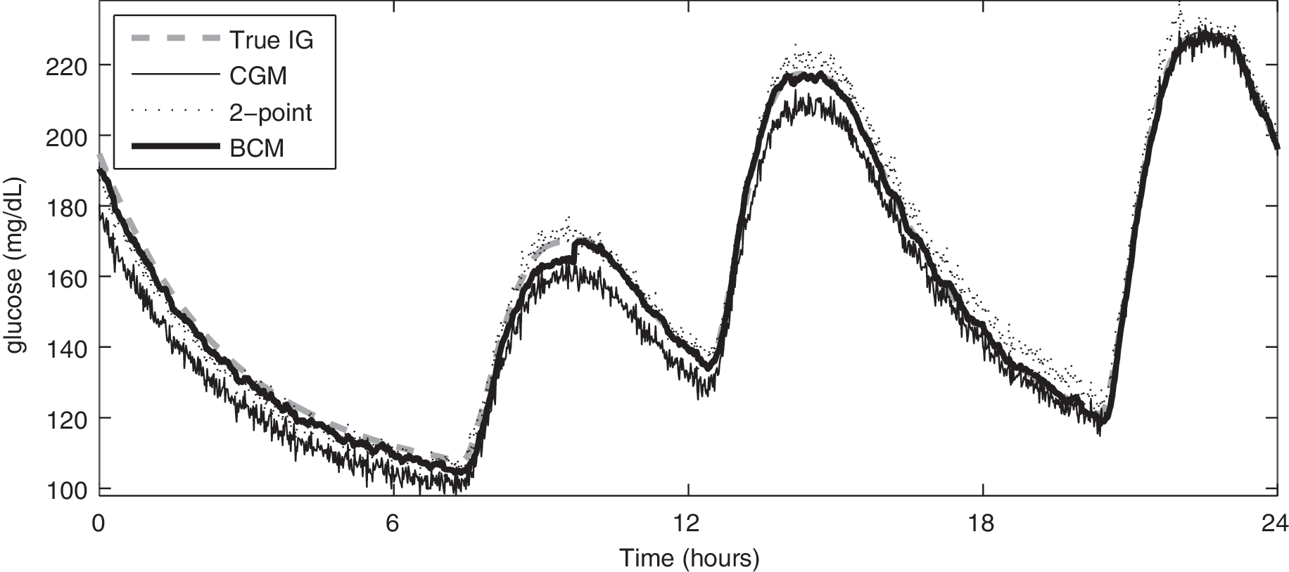
Subject number 3, detail of Day 6: true IG profile (gray dashed), CGM data (black thin), two-point calibrated (black dotted), and BCM enhanced (black thick) CGM profiles.

Robustness to suboptimal SMBG scheduling

In this subsection we investigate the situation in which a suboptimal scheduling of the four SMBG measurements per day is provided. In particular, each of the four SMBG samples per day is collected randomly in a time interval of 30 min centered at the “optimal” sampling times used in the previous simulations. Columns 4 and 5 of Table 2 report the RMSE for this first simulation. Also in this case, BCM performs much better than the two-point method, with a significant reduction of the RMSE of 43% (P < 0.01). Notably, BCM performance is almost insensitive to the suboptimality of SMBG sampling (+3%, comparing average results of columns 1 and 4), whereas the two-point procedure has a significant decrease in performance (+21%, comparing average results of columns 3 and 5). In order to stress the performance of BCM, a second test has been performed by increasing the time interval to 2 h. RMSE values are reported in columns 6 and 7 for BCM and the two-point procedure, respectively. The BCM mean RMSE increases of only 5.4% if compared to results of optimal scheduling (3.7 vs. 3.5, respectively) and, not surprisingly, is significantly better than the two-point calibration in terms of RMSE (71%, P < 0.001). In addition, by looking at SD values, RMSE variability from subject to subject is similar to the ideal situation only for BCM.

Robustness to reduction of SMBG measurements

It is of interest to test the performance of BCM by reducing the number of SMBG samples exploited. In particular, a new SMBG scheduling has been drawn in which only two measurements per day are provided. The two samples have been collected one at breakfast and one at the postprandial dinner peak, respectively, and both with suboptimal timing (randomly taken in the 2-h window around each point). For each subject RMSE values are reported in the last column of Table 2. By looking at the results it is evident that even if resorting only to two SMBG samples per day, BCM mean RMSE increases by only 33% if compared to results of four SMBG samples with optimal scheduling. This confirms that BCM is able to perform satisfactorily also in suboptimal conditions concerning both number and scheduling of SMBG samples.

Finally, we also tested the performance of BCM by applying higher CV values to SMBG measurements and obtained results comparable to the ones presented above (data not shown).

Robustness to errors in τ

We also investigated the influence of the value of τ in Eq. 7. The value of τ can significantly vary from subject to subject,¹⁵ and its individual identification is impossible in practice because it would require abundant BG references per day.

The first simulation is aimed to test BCM if, inside the model, a wrong τ value is used. In particular, we choose τ values from 6 to 18 min, i.e., we consider the worst case in which the BG-to-IG model has 50% of error. Figure 7 shows the BCM average RMSE values (black profile) obtained comparing true IG and enhanced CGM time series. Even in the worst case, i.e., by using τ = 6 min, BCM performance in terms of RMSE is better than for the two-point method (3.9 vs. 5.2, respectively). If compared with the result of the optimal SMBG scheduling of section (see BCM on simulated data) (average RMSE = 3.5), the average RMSE increases only by 12%. This means that, even if we use inside BCM a τ value that is lower/greater than 50% of the real one, BCM still performs better than the calibration procedure of King et al.¹⁷

FIG. 7.

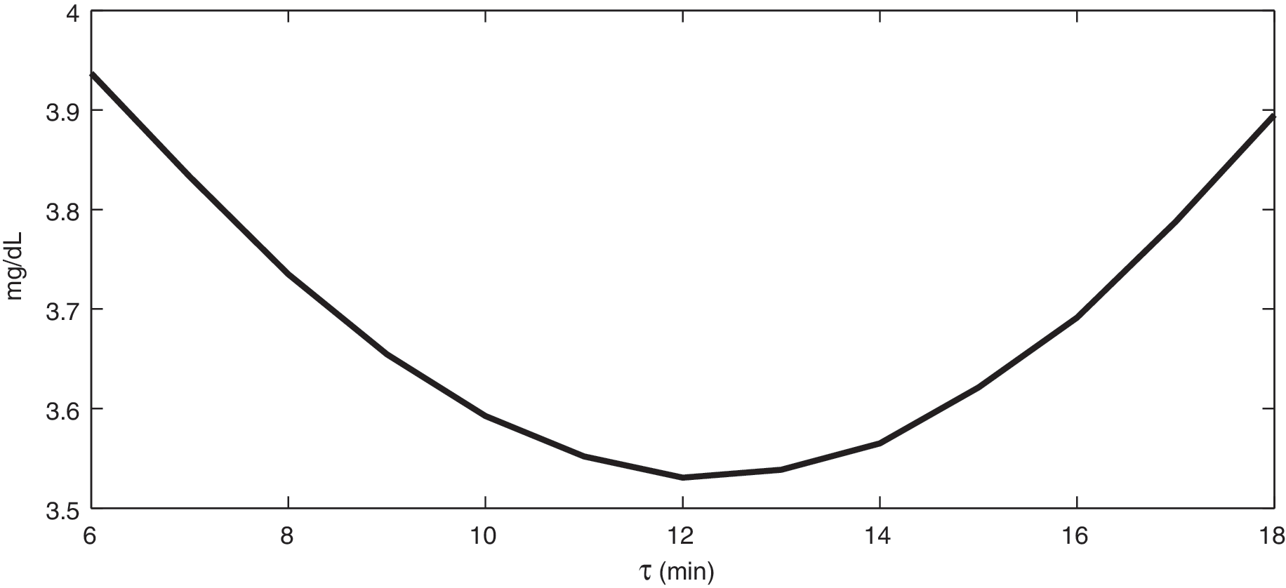
The average BCM RMSE obtained comparing true IG versus enhanced CGM time series by using a wrong τ value in the BG-to-IG kinetics model (±50% of the true value, i.e., 12 min).

In the second simulation, we compared the performance of individualized versus “population” BCM. The dataset created in Simulated Database has been modified in order to take into account the interindividual variability of τ. Ten new simulated subjects have been created, each one with a different τ drawn from a Gaussian distribution (18 ± 4 min [see Facchinetti et al.¹⁵]). The mean and SD values of the RMSE were 3.6 ± 1.1 and 4.1 ± 1.4 mg/dL, by using the individualized and the “population” BCM, respectively. This result evidences that BCM, even with “population” parameters, performs satisfactorily.

BCM on a representative subject

BCM was also tested on the same subject of Figure 1. As one can see by comparing the two time series, the CGM profile is characterized by an evident underestimation of the glycemic level in the time interval 17–21 h. Two of the BG references have been selected to simulate two SMBG measurements (see the gray circles plotted in the top panel of Fig. 8). Then, BCM has been applied as data were received in real time. By looking at the results, a zoom of which is shown in Figure 8, not only has the underestimation of the original CGM data been correctly identified by estimating a negative value of α in correspondence to the time window 15–21 h (bottom panel), but also it has been satisfactorily recovered. In fact, the enhanced CGM profile (black series in the top panel) presents increased CGM values exactly in that window if compared to the original one. Quantitatively, the RMSE calculated in 18–26 h, i.e., after the two SMBG samples have been exploited, between BG references (we remember not used by BCM) and CGM profile has been reduced from 32.0 to 25.5 mg/dL thanks to the enhanced calibration.

FIG. 8.

Representative real subject. (Top) Measured (gray) versus enhanced (black) CGM time series as well as SMBG samples (gray circles). (Bottom) Estimated α profile.

Conclusions

In this work we have proposed a new online enhanced calibration method that can be applied in cascade to the standard CGM device calibration in order to improve the accuracy of CGM output. This method, which is an improvement of the algorithm of Knobbe and Buckingham,¹¹ is embedded within a stochastic framework and implemented by EKF. By taking into account BG-to-IG kinetics, few SMBG samples per day, and a model describing the sensor gain variability, the enhanced calibration method significantly improves the accuracy of CGM data in real-time. Furthermore, the method intrinsically denoises the CGM signal and, as a by-product, also provides a continuous-time estimate of both BG and sensor gain.

Compared to state of art literature calibration strategy, the new method performs significantly better, when both optimal and suboptimal scheduling of the four SMBG measurements is done and when the number of the SMBG per day is reduced. Also, the method exhibits small sensitivity to variations of the BG-to-IG time constant τ. In addition, when applied to a real dataset, BCM is shown to correctly identify under- and overestimations of original CGM profile and to improve sensor outcome.

Finally, we note that the application of the BCM to real data requires the knowledge of the variances of both state and measurement processes, which in real-life conditions are usually unknown. Therefore, a real-time method for this estimation should be considered. Another aspect is related to the need of a burn-in interval. Here, 1 day was exploited in order to estimate the covariance matrix of the state vector in the transient phase.

In conclusion, the enhanced calibration algorithm significantly improves the accuracy of CGM signals, suggesting that it could be profitably included in real-time applications of CGM devices, e.g., algorithms for open/closed-loop diabetes control. The model here used for the description of the sensor gain deviation α is rather general and could be used in cascade to make an enhanced calibration for any CGM device. In addition, the method could be also used retrospectively to efficiently improve the accuracy of CGM profiles before applying to those data any type of post-processing.

Footnotes

Acknowledgments

We thank Dr. Chiara Dalla Man (University of Padova, Padova, Italy) for having provided the software^13,20,21 and for her helpful support in its use in the simulations reported in the present work.

Author Disclosure Statement

The authors have no conflicts of interest.

References

Nichols

, Klonoff

. The need for performance standards for continuous glucose monitors. J Diabetes Sci Technol, 2007; 1:92–95.

Block C

, Vertommen

, Manuel-y-Keenoy

, Van Gaal

. Minimally-invasive and non-invasive continuous glucose monitoring systems: indications, advantages, limitations and clinical aspects. Curr Diabetes Rev, 2008; 4:159–168.

Garg

, Zisser

, Schwartz

, Bailey

, Kaplan

, Ellis

, Jovanovic

. Improvement in glycemic excursions with a transcutaneous, real-time continuous glucose sensor. Diabetes Care, 2006; 29:44–50.

Klonoff

. Continuous glucose monitoring: roadmap for 21st century diabetes therapy. Diabetes Care, 2005; 28:1231–1239.

Battelino

, Bolinder

. Clinical use of real-time continuous glucose monitoring. Curr Diabetes Rev, 2008; 4:218–222.

Simpson

, Brister

, Wightlin

, Pryor

. inventors; DexCom, Inc., assignee. Dual electrode system for a continuous analyte sensor. Publication Number WO/2008/042918; April 10, 2008. International Application Number PCT/US2007/080228, October 4, 2007.

Feldman

, McGarraugh

. inventors; Abbott Diabetes Care, Inc., assignee. Method of calibrating an analyte-measurement device, and associated methods, devices and systems. U.S. Patent 7,299,082, November 20, 2007.

Mastrototaro

, Gross

, Shin

. inventors; Medtronic Minimed, Inc., assignee. Glucose monitor calibration methods. U.S. Patent 6,424,847, July 23, 2002.

Kovatchev

, Gonder-Frederick

, Cox

, Clarke

. Evaluating the accuracy of continuous glucose-monitoring sensors: continuous glucose-error grid analysis illustrated by TheraSense Freestyle Navigator data. Diabetes Care, 2004; 27:1922–1928.

10.

Rebrin

, Steil

, van Antwerp

. Subcutaneous glucose predicts plasma glucose independent of insulin: implications for continuous monitoring. Am J Physiol, 1999; 277:E561–E571.

11.

Knobbe

, Buckingham

. The extended Kalman filter for continuous glucose monitoring. Diabetes Technol Ther, 2005; 7:15–27.

12.

Magni

, Raimondo

, Bossi

, Dalla

Man C

, De

Nicolao G

, Kovatchev

, Cobelli

. Model predictive control of type 1 diabetes: an in silico trial. J Diabetes Sci Technol, 2007; 1:804–812.

13.

Kovatchev

, Breton

, Dalla

Man C

, Cobelli

. In silico preclinical trials: a proof of concept in closed-loop control of type 1 diabetes. J Diabetes Sci Technol, 2009; 3:44–55.

14.

Diabetes Research in Children Network (Direcnet) Study Group. Buckingham

, Kollman

, Beck

, Kalajian

, Fiallo-Scharer

, Tansey

, Fox

, Wilson

, Weinzimer

, Ruedy

, Tamborlane

. Evaluation of factors affecting CGMS calibration. Diabetes Technol Ther, 2006; 8:318–325.

15.

Facchinetti

, Sparacino

, Cobelli

. Reconstruction of glucose in plasma from interstitial fluid continuous glucose monitoring data: role of sensor calibration. J Diabetes Sci Technol, 2007; 1:617–623.

16.

Breton

, Kovatchev

. Analysis, modeling, and simulation of the accuracy of continuous glucose sensors. J Diabetes Sci Technol, 2008; 2:853–862.

17.

King

, Anderson

, Breton

, Clarke

, Kovatchev

. Modeling of calibration effectiveness and blood-to-interstitial glucose dynamics as potential confounders of the accuracy of continuous glucose sensors during hyperinsulinemic clamp. J Diabetes Sci Technol, 2007; 1:317–322.

18.

Lodwig

, Heinemann

. Glucose Monitoring Study Group. Continuous glucose monitoring with glucose sensors: calibration and assessment criteria. Diabetes Technol Ther, 2003; 5:572–586.

19.

Kuure-Kinsey

, Palerm

, Bequette

. A dual-rate Kalman filter for continuous glucose monitoring. Conf Proc IEEE Eng Med Biol Soc, 2006; 1:63–66.

20.

Dalla Man

, Raimondo

, Rizza

, Cobelli

. GIM, simulation software of meal glucose-insulin model. J Diabetes Sci Technol, 2007; 1:323–330.

21.

Dalla Man

, Rizza

, Cobelli

. Meal simulation model of the glucose-insulin system. IEEE Trans Biomed Eng, 2007; 54:1740–1749.

22.

Kovatchev

, Clarke

, Breton

, Brayman

, McCall

. Quantifying temporal glucose variability in diabetes via continuous glucose monitoring: mathematical methods and clinical application. Diabetes Technol Ther, 2005; 7:849–862.

23.

Chase

, Hann

, Jackson

, Lin

, Lotz

, Wong

, Shaw

. Integral-based filtering of continuous glucose sensor measurements for glycaemic control in critical care. Comput Methods Programs Biomed, 2006; 82:238–247.

24.

Nicolao G

, Sparacino

, Cobelli

. Nonparametric input estimation in physiological systems: problems, methods and case study. Automatica, 1997; 33:851–870.

25.

Facchinetti

, Sparacino

, Cobelli

. An on-line self-tuneable method to denoise CGM sensor data. IEEE Trans Biomed Eng, 2010; 57:634–641.

26.

http://glucosecontrol.ucsd.edu. 2009 April 1.

27.

Anderson

BDO

, Moore

. Optimal Filtering. Dover Publications: Mineola, NY, 2005.

28.

Grewal

, Andrews

. Kalman Filtering: Theory and Practice Using MATLAB. John Wiley and Sons: New York, 2001.