A Dynamic Risk Measure from Continuous Glucose Monitoring Data

Abstract

Background:

The quantitative analysis of glucose time-series can greatly help the management of diabetes. In particular, a static nonlinear transformation, which symmetrizes the distribution of glucose levels by bringing them in the so-called risk space, was proposed previously for both self-monitoring blood glucose and continuous glucose monitoring (CGM) and extensively used in the literature. The continuous nature of CGM data allows us to further refine the risk space concept in order to account for glucose dynamics.

Methods:

A new dynamic risk (DR) is proposed to explicitly consider the rate of change of glucose as a threat factor for the patient (e.g., risk levels in hypoglycemia and hyperglycemia are amplified in the presence of a decreasing and increasing glucose trend, respectively). The practical calculation of DR is made possible by the use of a regularized deconvolution algorithm that is able to deal with noise in CGM data and with the ill-conditioning of the time-derivative calculation, even in online applications.

Results:

Results on simulated and real data show that DR can be effectively computed and fruitfully used in real time (e.g., to generate early warnings of hypo-/hyperglycemic threshold crossings). Further applications of DR in the quantification of the efficiency of glucose control are also suggested.

Conclusions:

Exploiting the information on glucose trends empowers the strength of risk measures in interpreting CGM time-series.

Introduction

T he comprehensive analysis of glucose time-series is of great importance for the quantitative understanding of the glucose–insulin system and may help the definition of the therapeutic actions needed to achieve optimal glucose control (see Cobelli et al.¹ and references quoted therein). The simplest method for monitoring the glycemic level is self-monitoring blood glucose (SMBG) (i.e., finger pricks performed by the patients, usually three or four times a day). The retrospective analysis of SMBG with variability measures (see Rodbard² for a recent review on variability measures and Greven et al.³ for an application) has been used in the last decades in order to extract critical information for the definition of an insulin-infusion therapy schedule. Recently, continuous glucose monitoring (CGM) devices have become available, which are able to provide a measure of the glycemia every 1–5 min, hence offering a much richer clinical insight for interpreting glucose dynamics^4
–6 and opening the possibility of developing online therapeutic tools such as generators of hypo-/hyperglycemic threshold crossings alarms^7,8 and the artificial pancreas,^1,9 provided that some crucial but challenging signal processing issues are properly dealt with.^10,11

It has been suggested by Kovatchev et al.¹² that the study of glucose concentration time-series should take into account that the glycemic range is asymmetric, with the “hypoglycemia range” much narrower than the “hyperglycemia range” with a much faster increase of health threats when moving deeper in the first versus the latter range. As an example, consider glucose levels of 40 mg/dL or 210 mg/dL: although the absolute distance from the hypo-/hyperglycemic threshold (70 and 180 mg/dL, respectively) is the same (30 mg/dL), the first level corresponds to a situation of severe hypoglycemia, whereas the second corresponds to mild hyperglycemia. In other words, the risk for the patient increases much faster in hypoglycemia than in hyperglycemia when moving below or above the hypo-/hyperglycemia threshold, respectively. Also, the distribution of glucose concentration values is skewed within the range. As a consequence, episodes of hypoglycemia associated with greater potential danger for the patient are not sufficiently emphasized and are outmatched by the numerous mild hyperglycemic events. This means that the role of a few glycemic values deep in the hypoglycemia zone (e.g., two very dangerous hypoglycemias at 40 mg/dL) would be obscured in simple statistical measures such as mean and SDs by a large number of mild hyperglycemias. In the literature, some attempts to overcome this peculiarity of the glycemic range have been made by computing variability or control indexes after mapping glucose concentration in a penalty score (e.g., the Glycemic Risk Assessment Diabetes Equation proposed by Hill et al.¹³ and the Index of Glycemic Control developed by Rodbard,^14,15 which are able to equally weight hypo- and hyperglycemic episodes) (see Rodbard² for a comprehensive recent review).

A widely accepted transformation of the glycemic measurement scale has been proposed by Kovatchev et al.¹² and extensively exploited for the so-called risk analysis^16
–18 (see Clarke et al.¹⁹ for a recent review). In this approach, a nonlinear transformation converts every single glucose reading into a “static” risk value, which puts more emphasis on values within the clinically critical regions of hypo- and hyperglycemia than in the safe region of normoglycemia. Further developments in the risk space, used for both SMBG and CGM data,^16,20 resorted to numerical indexes—the Low and the High Blood Glucose Index—to quantify the tendency of a patient to stay in the hypo- or hyperglycemic region. These indexes have been found to correlate with the number of observed episodes of severe hypoglycemia and of hyperglycemia.¹⁶ Recently, a controller exploiting different weights in hypo-/hyperglycemic regions according to a risk function was proposed²¹ in order to account for the different clinical risks associated with different glucose levels.

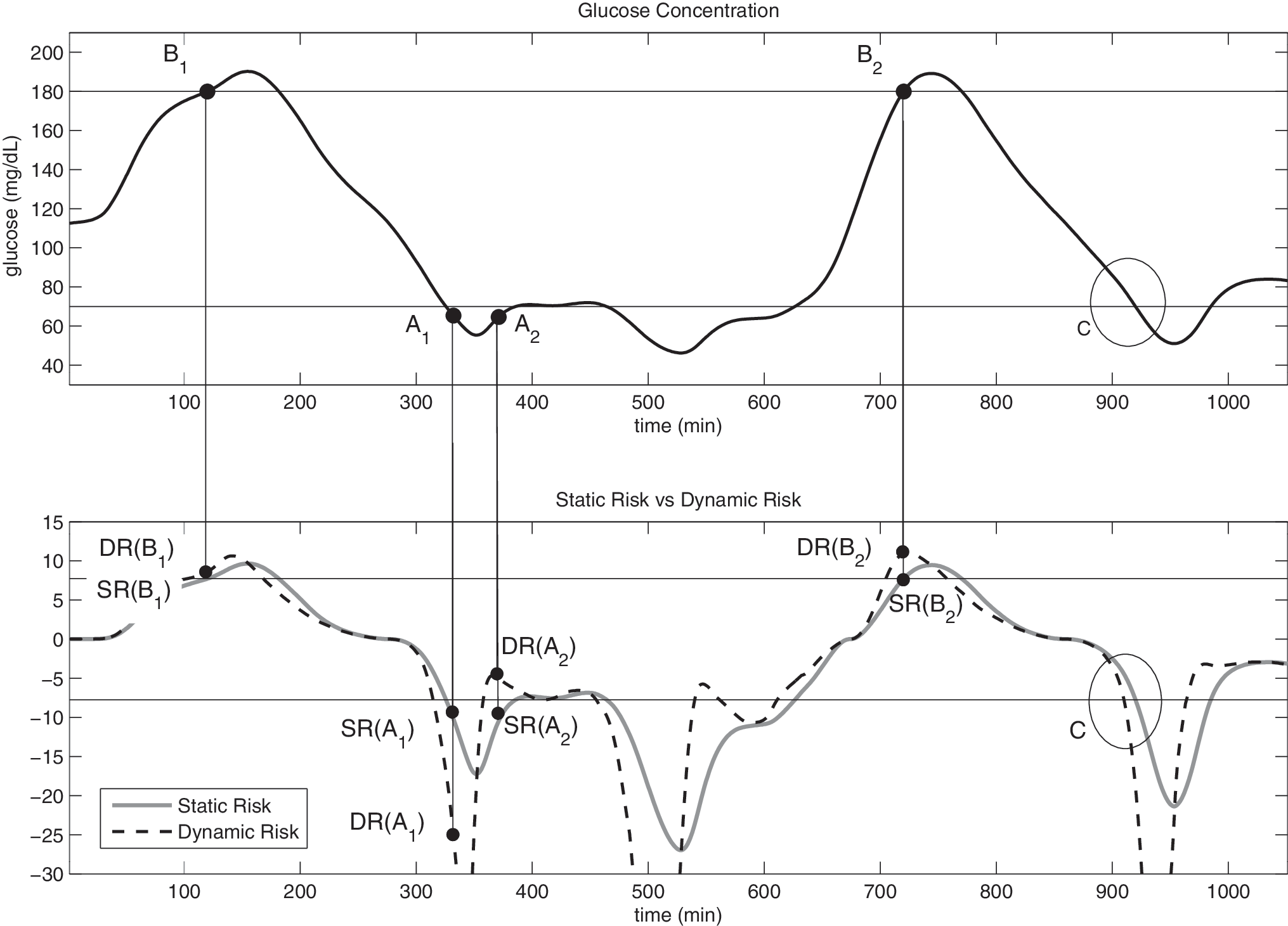
The above-mentioned transformations of glucose levels and the correspondent indexes are “static” (i.e., a given glycemic level is associated with a specific penalty or risk score). This was a natural step because these transformations were originally conceived for SMBG, where information about glucose trend is unavailable. Today, the availability of CGM signals opens the possibility of embedding glucose dynamics information in the evaluation of risk measures. Consider the example reported in Figure 1, which displays a simulated continuous glucose profile for 1,000 min. The picture highlights four particular points, labeled as A₁, A₂, B₁, and B₂, together with a portion of the tangent line to the glucose profile in these points. In addition, the circle labeled as C highlights an hypoglycemia threshold crossing event. It is notable that A₁ and A₂ correspond to a glucose concentration just below the hypoglycemia threshold (65 mg/dL) but with different derivatives (−2 mg/dL/min for A₁ and +2 mg/dL/min for A₂), whereas B₁ and B₂ are both placed exactly on the hyperglycemia threshold (180 mg/dL with derivatives of +2 mg/dL/min and +4 mg/dL/min, respectively). If only SMBG were available and using, for example, the function of Kovatchev et al.,¹² points A₁ and A₂ would be associated with the same risk value, and so would B₁ and B₂.

FIG. 1.

Simulated noise-free continuous glucose profile (continuous line) with hypo-/hyperglycemia thresholds (horizontal lines). Four points (dots) are indicated: A₁ and A₂ (65 mg/dL, decreasing and increasing trend, respectively) and B₁ and B₂ (180 mg/dL, rate of change of +2 mg/dL/min and +4mg/dL/min, respectively) with the correspondent tangent (thin line). Circle C highlights a hypoglycemic threshold crossing event.

However, by considering the continuous glucose profile of Figure 1, one easily realizes that the clinical risk associated with points A₁ and A₂ should be different. In fact, the A₁ situation is more dangerous for the patient than A₂ because in the first case the glycemia is heading deeper in the hypoglycemic region, whereas in the second case a recovering from the hypoglycemia region toward the normoglycemic range is happening. Similarly, the B₂ situation is more dangerous than B₁ because the glycemic signal is approaching the hyperglycemic region faster.

The above examples make it clear that the trend in the glycemia, which can be inferred from CGM measurements, should be considered in the risk measure. This is the goal of the present article. In particular, starting from the original risk function by Kovatchev et al.,¹² in the next section we will define a dynamic risk (DR) measure, dependent on both level and trend (measured as the first time-derivative) of actual glucose. The explicit inclusion of glucose trends in the definition of DR will call for an efficient and stable algorithm able to deal with the noise present in the CGM data (which renders the time-derivative calculation difficult because of ill-conditioning). This task will be tackled by exploiting a regularized deconvolution algorithm that is also usable to compute DR in online applications. Results on simulated and real data discussed in the following two sections will show that DR can be effectively computed and fruitfully used in real time (e.g., to generate early warnings of hypo-/hyperglycemic threshold crossings). Further applications of DR in the quantification of the efficiency of glucose control are also suggested in the discussion that concludes the article.

The DR

Rationale and requisites

Let's start by recalling the methodology proposed by Kovatchev et al.,¹² where, given a generic glycemic level g, the standard risk function r(g) is defined as \documentclass{aastex}\usepackage{amsbsy}\usepackage{amsfonts}\usepackage{amssymb}\usepackage{bm}\usepackage{mathrsfs}\usepackage{pifont}\usepackage{stmaryrd}\usepackage{textcomp}\usepackage{portland, xspace}\usepackage{amsmath, amsxtra}\pagestyle{empty}\DeclareMathSizes{10}{9}{7}{6}\begin{document} \begin{align*} r (g) = 10 \cdot f (g) ^2 \tag{1} \end{align*} \end{document}

where \documentclass{aastex}\usepackage{amsbsy}\usepackage{amsfonts}\usepackage{amssymb}\usepackage{bm}\usepackage{mathrsfs}\usepackage{pifont}\usepackage{stmaryrd}\usepackage{textcomp}\usepackage{portland, xspace}\usepackage{amsmath, amsxtra}\pagestyle{empty}\DeclareMathSizes{10}{9}{7}{6}\begin{document} \begin{align*} f (g) = \gamma \cdot [(\ln (g))^{\alpha} - \beta] \tag{2} \end{align*} \end{document}

with α, β, and γ being scalars equal to 1.084, 5.381, and 1.509 (assuming glucose expressed in mg/dL). The above function r(g) maps the glycemic range (20 ÷ 600) mg/dL to the (static) risk space range (0 ÷ 100). From r(g), two quantities, the low and high glucose risk, r _l(g) and r _h(g), respectively, are defined as \documentclass{aastex}\usepackage{amsbsy}\usepackage{amsfonts}\usepackage{amssymb}\usepackage{bm}\usepackage{mathrsfs}\usepackage{pifont}\usepackage{stmaryrd}\usepackage{textcomp}\usepackage{portland, xspace}\usepackage{amsmath, amsxtra}\pagestyle{empty}\DeclareMathSizes{10}{9}{7}{6}\begin{document} \begin{align*} r_{\rm l} (g) = \begin{cases}r (g) \quad{\rm if} \ f (g) < 0 \\ \quad 0 \quad {\rm otherwise}\end{cases} \\ r_{\rm h} (g) = \begin{cases}r (g) \quad {\rm if} \ f (g) > 0 \\ \quad 0 \quad {\rm otherwise}\end{cases} (3) \end{align*} \end{document}

In order to distinguish the situations A₁ versus A₂ and B₁ versus B₂ of Figure 1, below we will modify the risk function of Eq. 1 and define a DR measure, DR, in order to take into account not only the actual glycemic level, but also its trend, measured by the first time-derivative. Conceptually this requires adoption of a DR of the form \documentclass{aastex}\usepackage{amsbsy}\usepackage{amsfonts}\usepackage{amssymb}\usepackage{bm}\usepackage{mathrsfs}\usepackage{pifont}\usepackage{stmaryrd}\usepackage{textcomp}\usepackage{portland, xspace}\usepackage{amsmath, amsxtra}\pagestyle{empty}\DeclareMathSizes{10}{9}{7}{6}\begin{document} \begin{align*} DR = \Phi \left( g , \frac {dg} {dt} \right) \tag {4} \end{align*} \end{document}

In particular, the functional Φ should be designed in order to have two desirable properties:

1. In stationary conditions (i.e., g is constant in time), the module of DR(g,0) should equal r(g), that is, \documentclass{aastex}\usepackage{amsbsy}\usepackage{amsfonts}\usepackage{amssymb}\usepackage{bm}\usepackage{mathrsfs}\usepackage{pifont}\usepackage{stmaryrd}\usepackage{textcomp}\usepackage{portland, xspace}\usepackage{amsmath, amsxtra}\pagestyle{empty}\DeclareMathSizes{10}{9}{7}{6}\begin{document} \begin{align*} DR (g , 0) = r (g) \tag{5} \end{align*} \end{document}

In this way, when glucose is stable, DR will equal the standard static risk (SR) r(g) of Eq. 1.

2. When glucose is moving toward critical hypo-/hyperglycemic regions, r(g) of Eq. 1 should be amplified, whereas it should be attenuated when g is approaching normoglycemia. This will be accomplished by choosing a function Φ such that \documentclass{aastex}\usepackage{amsbsy}\usepackage{amsfonts}\usepackage{amssymb}\usepackage{bm}\usepackage{mathrsfs}\usepackage{pifont}\usepackage{stmaryrd}\usepackage{textcomp}\usepackage{portland, xspace}\usepackage{amsmath, amsxtra}\pagestyle{empty}\DeclareMathSizes{10}{9}{7}{6}\begin{document} \begin{align*} \begin{cases}DR > r (g) \quad {\rm if} \quad \frac {dg} {dt} \cdot SR (g) > 0 \\ DR < r (g) \quad {\rm if} \quad \frac {dg} {dt} \cdot SR (g) < 0 \end{cases} \tag {6} \end{align*} \end{document}

where SR(g) is defined in the present article as \documentclass{aastex}\usepackage{amsbsy}\usepackage{amsfonts}\usepackage{amssymb}\usepackage{bm}\usepackage{mathrsfs}\usepackage{pifont}\usepackage{stmaryrd}\usepackage{textcomp}\usepackage{portland, xspace}\usepackage{amsmath, amsxtra}\pagestyle{empty}\DeclareMathSizes{10}{9}{7}{6}\begin{document} \begin{align*} SR (g) = r_{\rm h} (g) - r_{\rm l} (g) \tag{7} \end{align*} \end{document}

and from now on will be referred to as SR. Note that SR(g) in Eq. 7 is equivalent to the original definition of risk given by Kovatchev et al.,¹² with the only difference that, when there is a hypoglycemia risk [i.e., f(g) < 0], the sign is changed.

Mathematical definition

In order to obey the requisites of points 1 and 2 in the preceding section, DR is defined as \documentclass{aastex}\usepackage{amsbsy}\usepackage{amsfonts}\usepackage{amssymb}\usepackage{bm}\usepackage{mathrsfs}\usepackage{pifont}\usepackage{stmaryrd}\usepackage{textcomp}\usepackage{portland, xspace}\usepackage{amsmath, amsxtra}\pagestyle{empty}\DeclareMathSizes{10}{9}{7}{6}\begin{document} \begin{align*} DR (g , \frac {dg} {dt}) = \begin{cases} SR (g) \cdot e^ {+ \mu \frac {dr} {dt}} \quad {\rm if} \quad SR (g) > 0 \\ SR (g) \cdot e^ {- \mu \frac {dr} {dt}} \quad {\rm if} \quad SR (g) < 0 \end{cases} \tag {8} \end{align*} \end{document}

where r is the function of g of Eq. 1 (for the sake of simplicity, the dependence on g is not explicitly evidenced) and the scalar μ is a tunable parameter that determines how much SR can be amplified or attenuated (see Assessment on Real Data for details). In Eq. 8, given the definition of Eq. 1, one can exploit the following expression: \documentclass{aastex}\usepackage{amsbsy}\usepackage{amsfonts}\usepackage{amssymb}\usepackage{bm}\usepackage{mathrsfs}\usepackage{pifont}\usepackage{stmaryrd}\usepackage{textcomp}\usepackage{portland, xspace}\usepackage{amsmath, amsxtra}\pagestyle{empty}\DeclareMathSizes{10}{9}{7}{6}\begin{document} \begin{align*} \frac {dr} {dt} = \frac {dr} {dg} \frac {dg} {dt} = \left\{ 10 \gamma^2 \cdot [(\ln (g))^{2 \alpha - 1} - \beta (\ln (g))^{\alpha - 1}] \cdot 2 \alpha \frac {1} {g} \right\} \cdot \frac {dg} {dt} \tag {9} \end{align*} \end{document}

with α, β, and γ equal to those defined for Eq. 2.

The function of Eq. 8 is the product of two factors: the static risk SR of Eq. 7 and an exponential component that has the role of risk amplifier/damper accordingly to the actual glycemic level and trend. In the design of Eq. 8, the exponential was selected because of its simplicity and because it meets requirements 1 and 2 of the preceding section. In fact, when the first time-derivative of g is 0, one has DR = SR, which is a condition equivalent to that of Eq. 5. Moreover as required by Eq. 6, if dr/dt and SR have different sign (i.e., either hypoglycemia with increasing trend or hyperglycemia with decreasing trend), the DR is given by SR·e ^−x with x > 0, and the risk decreases. On the other hand, if glycemia is heading very steeply toward euglycemia, the risk drops to 0.

Intuitively summarizing, the idea is multiplying SR, which is an indicator of the glycemic level and will be negative in hypoglycemia and positive in hyperglycemia, by a term (the exponential in this case) that depends on the trend. The latter term is greater than 1—acting as a risk amplifier—if the glucose trend is leading the patient to a dangerous zone (e.g., increasing trend in a hyperglycemic zone or decreasing trend in a hypoglycemic zone) and less than 1—acting as a damper—if the trend leads the patient to exiting a dangerous situation.

Numerical implementation

DR assumes that both glucose profile g(t) and its time-derivative are available. In practical cases the calculation of DR must be done from noisy glucose samples. In particular, with real CGM signals, the estimation of the first derivative of the glucose signal is difficult because high frequency noise present in the data will eventually be amplified by a differentiation operation because of ill-conditioning. In this work, we deal with this difficulty by estimating the first derivative through a regularized deconvolution approach. In fact, denoting by u(t) the time-derivative of the glucose signal \documentclass{aastex}\usepackage{amsbsy}\usepackage{amsfonts}\usepackage{amssymb}\usepackage{bm}\usepackage{mathrsfs}\usepackage{pifont}\usepackage{stmaryrd}\usepackage{textcomp}\usepackage{portland, xspace}\usepackage{amsmath, amsxtra}\pagestyle{empty}\DeclareMathSizes{10}{9}{7}{6}\begin{document} \begin{align*} u (t) = \frac {dg (t)} {dt} \tag {10} \end{align*} \end{document}

it holds \documentclass{aastex}\usepackage{amsbsy}\usepackage{amsfonts}\usepackage{amssymb}\usepackage{bm}\usepackage{mathrsfs}\usepackage{pifont}\usepackage{stmaryrd}\usepackage{textcomp}\usepackage{portland, xspace}\usepackage{amsmath, amsxtra}\pagestyle{empty}\DeclareMathSizes{10}{9}{7}{6}\begin{document} \begin{align*} g (t) = \int_{- \infty}^{t} u (\tau) d \tau \tag{11} \end{align*} \end{document}

which can be rewritten as \documentclass{aastex}\usepackage{amsbsy}\usepackage{amsfonts}\usepackage{amssymb}\usepackage{bm}\usepackage{mathrsfs}\usepackage{pifont}\usepackage{stmaryrd}\usepackage{textcomp}\usepackage{portland, xspace}\usepackage{amsmath, amsxtra}\pagestyle{empty}\DeclareMathSizes{10}{9}{7}{6}\begin{document} \begin{align*} g (t) = \int_{- \infty}^{t} h (t - \tau) u (\tau) d \tau = (h*u) (t) \tag{12} \end{align*} \end{document}

where h(t) is the unitary step function.²² The deconvolution problem of reconstructing u(t) of Eq. 10 from noisy samples of g(t) of Eq. 12 may be solved by a regularization technique, as explained in De Nicolao et al.,²³ to which we refer the reader for details. To permit online applications of DR, the deconvolution procedure can be repeated at any sampling time. Here, in particular, the deconvolution approach²³ is performed by considering a sliding window of 2-h past data, the regularization criterion therein indicated as ML2, and a penalty functional of order 1. It is notable that regularization also returns a smoothed version of the glucose profile g(t), which is exploited in the numerical calculation of DR by Eq. 8.

Assessment on Simulated Data

Data generation

Simulated continuous glucose profiles of 4 days of average duration were obtained from the smoothing spline interpolation of 10 frequently sampled blood glucose time-series taken from a previously published database available on the web (glucosecontrol.ucsd.edu/data.html). A portion of a representative glucose profile, limited to 1,000 min and already reported in Figure 1, is displayed again for picture completeness, in Figure 2, top panel. DR will be computed simulating real-time conditions and compared with SR, both in the ideal case of noise-free data (Assessment on noise-free data) and in a realistic case in which measurement error, simulating that of CGM devices, is present (Assessment on noisy data).

FIG. 2.

(Top panel) Same simulated noise-free glucose profile of Figure 1. (Bottom panel) Static risk (SR) (gray) and dynamic risk (DR) (dashed black). DR and SR of the highlighted conditions on the top panel are shown as black dots in the bottom panel. The circle highlights the anticipation in threshold crossing of DR with respect to SR in event C. The horizontal lines represent the threshold crossings transformed in the risk scale.

Assessment on noise-free data

Figure 2, bottom panel, shows a representative example of SR (solid line) versus DR (dashed line). The horizontal lines represent the transformation of the hypo- and hyperglycemic thresholds in the risk domain exploiting the SR definition. DR is calculated with μ = 2.2 in Eq. 8 (see Remark 1 below). Although SR does not distinguish between A₁ and A₂, DR for A₁ is lower than for A₂. This agrees with the perception of health danger associated with the two situations in which the first (i.e., hypoglycemia with negative trend) is much more threatening than the second (i.e., transition from hypoglycemia to euglycemia). In the same way, although SR gives the same risk to B₁ and B₂, DR is able to point out that the B₂ condition is more risky than B₁ because the same hyperglycemic value is associated to a positive greater rate of change in the glucose signal.

A very interesting feature of DR is that, being the trend of the glucose signal explicitly incorporated in it, it can be used to infer for the future in the short term. For example, DR may be exploited to predict hypo-/hyperglycemia threshold crossings with some minutes of advance. This can be seen by looking at the threshold crossings in Figure 2, bottom panel. In particular, for the event labeled as C, DR anticipates the threshold crossing by 10 min with respect to SR. On the 10 simulated noise-free data, where a total of 73 and 61 hypo- and hyperglycemic events were present, respectively, the median anticipation of the threshold crossing was 12 min (11.99 ± 3.16, mean ± SD).

Assessment on noisy data

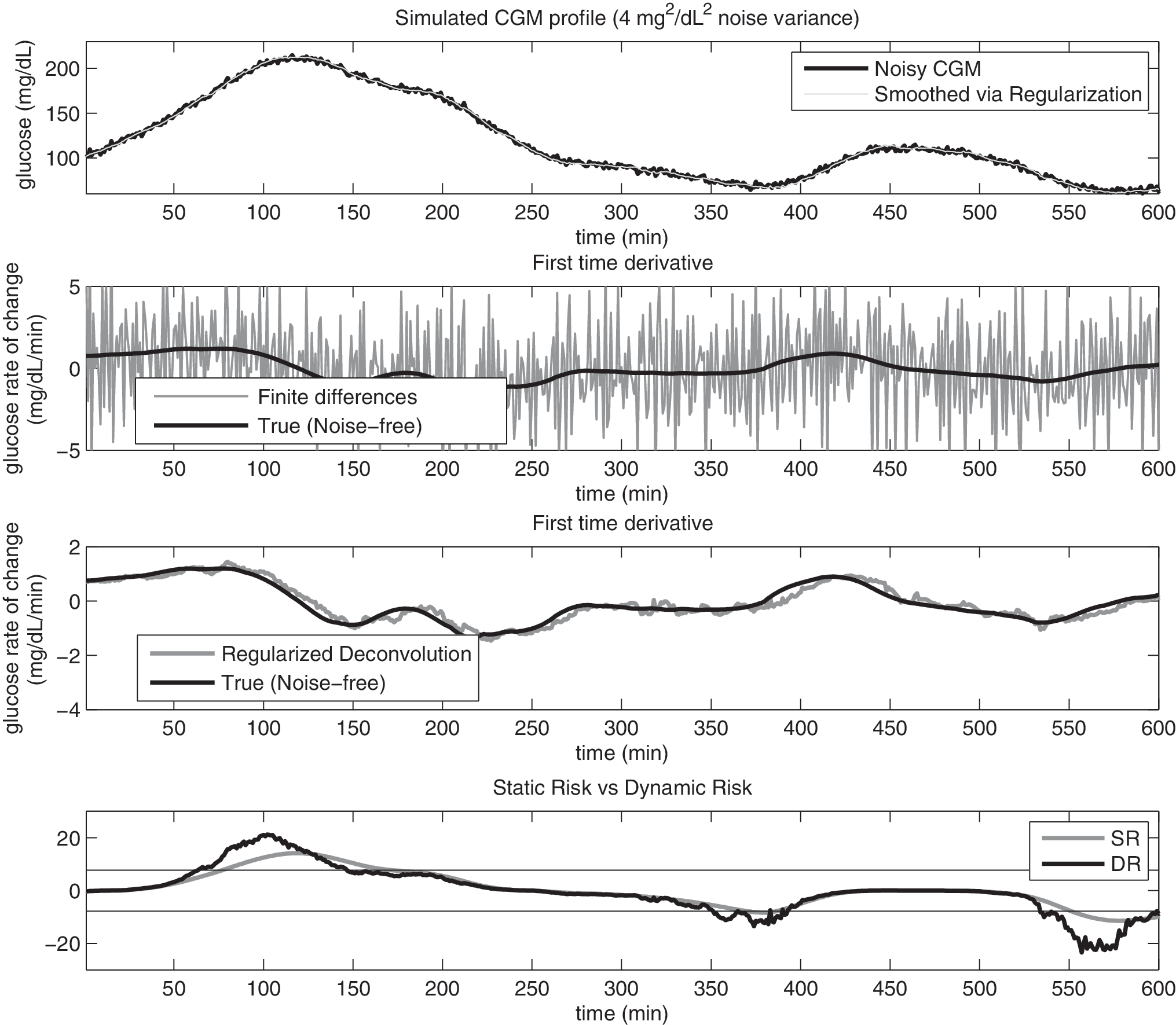
In order to assess DR in more realistic conditions, Gaussian zero mean white noise with variance equal to 4 mg²/dL² was added to the simulated glucose profiles generated in Data generation to mimic measurement noise of CGM time-series.²⁴ The top panels of Figures 3 and 4 show two representative examples of simulated CGM signals obtained from the same noise-free profile (not shown for clarity of the picture), but with two different superimposed noise realizations with variance 4 and 16 mg²/dL², respectively (black line). The smoothed glucose profile, obtained as a by-product of the regularized deconvolution procedure of Numerical implementation, is also shown in the top panel (gray line). In the middle panels we report the true (black) versus the estimated first time-derivative (gray line) obtained with conventional first-order finite differences (upper middle) and via the regularized deconvolution method of Numerical implementation (lower middle). Even in presence of high noise (Fig. 4), the regularized deconvolution approach allows a very satisfactory causal reconstruction of both the glucose signal and its first time-derivative, allowing the computation of a relatively smooth DR signal, reported in the lower panel (black) together with SR (gray line). Both Figures 3 and 4 demonstrate that practical (online) calculation of DR would be, however, impossible without proper dealing with the ill-conditioning of time-derivative estimation. In fact, the error present in the estimates provided by first-order finite differences (second panels) is an order of magnitude larger than the target (especially in Fig. 4).

FIG. 3.

(Top panel) Reconstructed continuous glucose monitoring (CGM) profile (gray line) and simulated noisy profile (black line). Variance of the Gaussian noise added to the signals was 4 mg²/dL². (Middle panels) First time-derivative calculated from the noise-free signal (black line) and estimated from the noisy signal via finite differences (upper middle, gray line) and regularization (lower middle, gray line). (Bottom panel) SR (gray line) versus DR (black line).

FIG. 4.

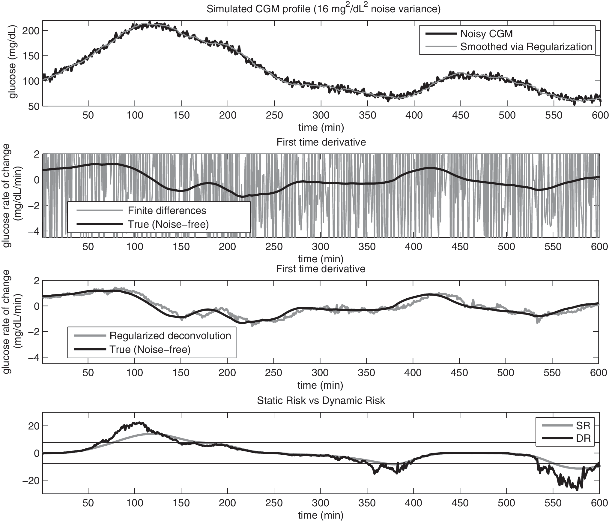
Same as Figure 3, but with variance of the Gaussian noise added to the signal equal to 16 mg²/dL². CGM, continuous glucose monitoring; DR, dynamic risk; SR, static risk.

As can be seen in Figures 3 and 4, even in the presence of noise, DR allows anticipation of the threshold crossing with respect to SR. The median anticipation of threshold crossings is 10 and 9 min, with 11.00 ± 5.94 and 9.59 ± 5.72 (mean ± SD) in the case of noise variance equal to 4 and 16 mg²/dL², respectively. Of course, in the presence of high noise, DR may present very rapid oscillations and can lead to some false-positive threshold crossings. When considering as true events only the threshold crossings generated by the noise-free CGM and evaluating the number of false-positives and true-positives generated by DR computed from noisy data (noise variance of 4 and 16 mg²/dL²), sensitivity was 88.79% and 89.30%, whereas specificity was 98.11% and 97.07%, respectively.

Assessment on Real Data

Six CGM time-series (1 min sampling) collected by using the Abbott (Alameda, CA) Freestyle Navigator™ and taken from a previously published study²⁵ were considered. Figure 5 shows 1 day of monitoring in a representative subject. In the top panel, the original CGM signal is depicted (gray line) versus the smoothed version of the same signal obtained with the approach of Numerical implementation simulating an online situation (black line). In the lower panel, SR evaluated from the smoothed CGM and DR evaluated exploiting also the estimated time-derivative are reported. DR is able to correctly anticipate the critical threshold crossings (see time 250 and 870). The average threshold crossing anticipation for DR is on the order of 9 min, and the generation of alarms (on a total of 25 events) was assessed as having 86.10% sensitivity and 98.73% specificity.

FIG. 5.

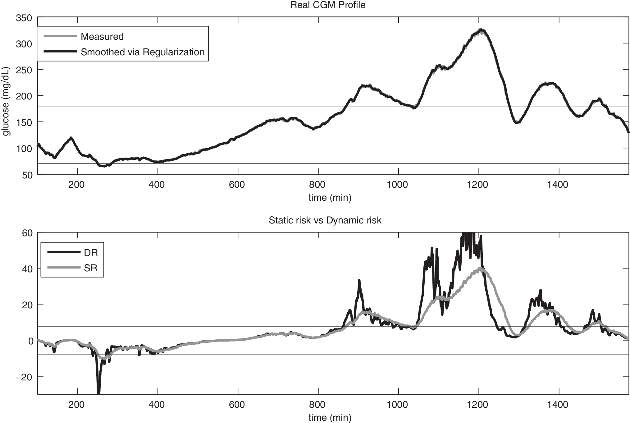
Dynamic risk (DR) assessed on real data. (Top panel) Measured continuous glucose monitoring (CGM) (gray line) and regularized estimate. (Lower panel) Static risk (SR) (gray line) versus dynamic risk (DR) (black line).

Remark 1: role of μ

In Eq. 8 the scalar μ determines how much SR can be amplified or attenuated in the determination of DR. Figure 6 shows a detail of SR (gray) and DR (black lines) of Figure 2. DR is computed with μ = 1, 2.2, and 4 (continuous, dashed, and dotted lines, respectively). It is notable that the amplification of the risk and the anticipation in the threshold crossing increase with μ. In practical cases a higher μ is expected to result in higher anticipation in threshold crossing and sensitivity of the hypo-/hyperglycemia alarms, but also in lower specificity of the hypo-/hyperglycemia alarms. Therefore the value of μ should be related to the signal-to-noise ratio in order to avoid spurious oscillations in the time-derivative to deteriorate the calculation of DR. In this article μ has been set to 2.2 because this value was retrospectively seen as a good compromise of mean anticipation in threshold crossing and percentage of false alerts. Also notice that μ = 0 implies DR = SR for any value of the time-derivative.

FIG. 6.
Role of μ: static risk (thick solid line) versus dynamic risk for the noise-free glucose profile of Figure 2 (top panel), where dynamic risk was calculated with μ = 1, μ = 2.2, and μ = 4 (black solid, dashed, and dotted lines, respectively).

Conclusions

The analysis of CGM time-series is of major importance for the management of diabetes with several online possible applications such as hypo-/hyperglycemia alarm generators and an artificial pancreas.³ The analysis of glucose time-series in the risk space, rather than simply considering glycemic levels per se, has been shown advantageous, and some indexes have been proposed, the most popular of which is the risk measure developed by Kovatchev et al.¹² In recent years, this static risk measure has been successfully applied, especially with SMBG samples. The continuous nature of CGM signals suggests that this static risk formulation can be empowered by also accounting for the trend of the signal.

In particular, in this article we have proposed a DR function, DR, that explicitly incorporates the rate of change of glucose as an amplifier/damper of the original SR originally defined by Kovatchev et al.¹² This means that a situation with a given hypoglycemic level with decreasing glucose concentration is quantified as more risky than the same hypoglycemic value with increasing glucose. Similarly, hyperglycemic levels in the presence of a rising glycemia (heading even to more severe hyperglycemic conditions) are considered more risky than the same hyperglycemic levels with falling glucose. This amplification/reduction of risk is obtained by multiply the standard transformation of the glucose scale proposed by Kovatchev et al.¹² by a term that explicitly considers the rate of change (trend). Practical challenges in the DR as implemented in this article (i.e., numerical calculation due to ill-conditioning of time-derivative calculation) have been dealt with by using a causal regularized deconvolution approach. The effectiveness of DR has been successfully tested on both simulated and real glucose CGM profiles.

DR has great potential for online use in algorithms for the generation of alarms for the prevention of glycemic shocks, as discussed in Assessment on Simulated Data and Assessment on Real Data. Further work will be carried on to investigate in detail the use of DR in prediction, in particular for the possibility of calculating DR of predicted time-series and comparing the results with different approaches (e.g., comparison with risk scores based on the integral of SR). Moreover, comparison with prediction algorithms (e.g., AR) will be performed, possibly evaluating SR of predicted signals as a term of comparison. A further possible use of DR, in both retrospective and online analysis of CGM signals, is suggested by Figure 7, where trajectories drawn by the pairs (g,dg/dt) are depicted, as proposed in Rahaghi and Gough.²⁶ Here in particular, we plot the module of DR as a function of glucose concentration and its first derivative in the DR space (DRS), where red regions are associated with higher clinical risk [values at derivative equal to 0 correspond to r(g)]. In the two plots, two subjects taken from the dataset used in Data generation are shown. It is notable that the trajectories in DRS show that the first subject is much better controlled than the second one, with a trajectory in DRS is more concentrated in the safe (green) zone. Possible exploitation of this concept to assess the quality of glucose control in real subjects is currently under investigation.

FIG. 7.
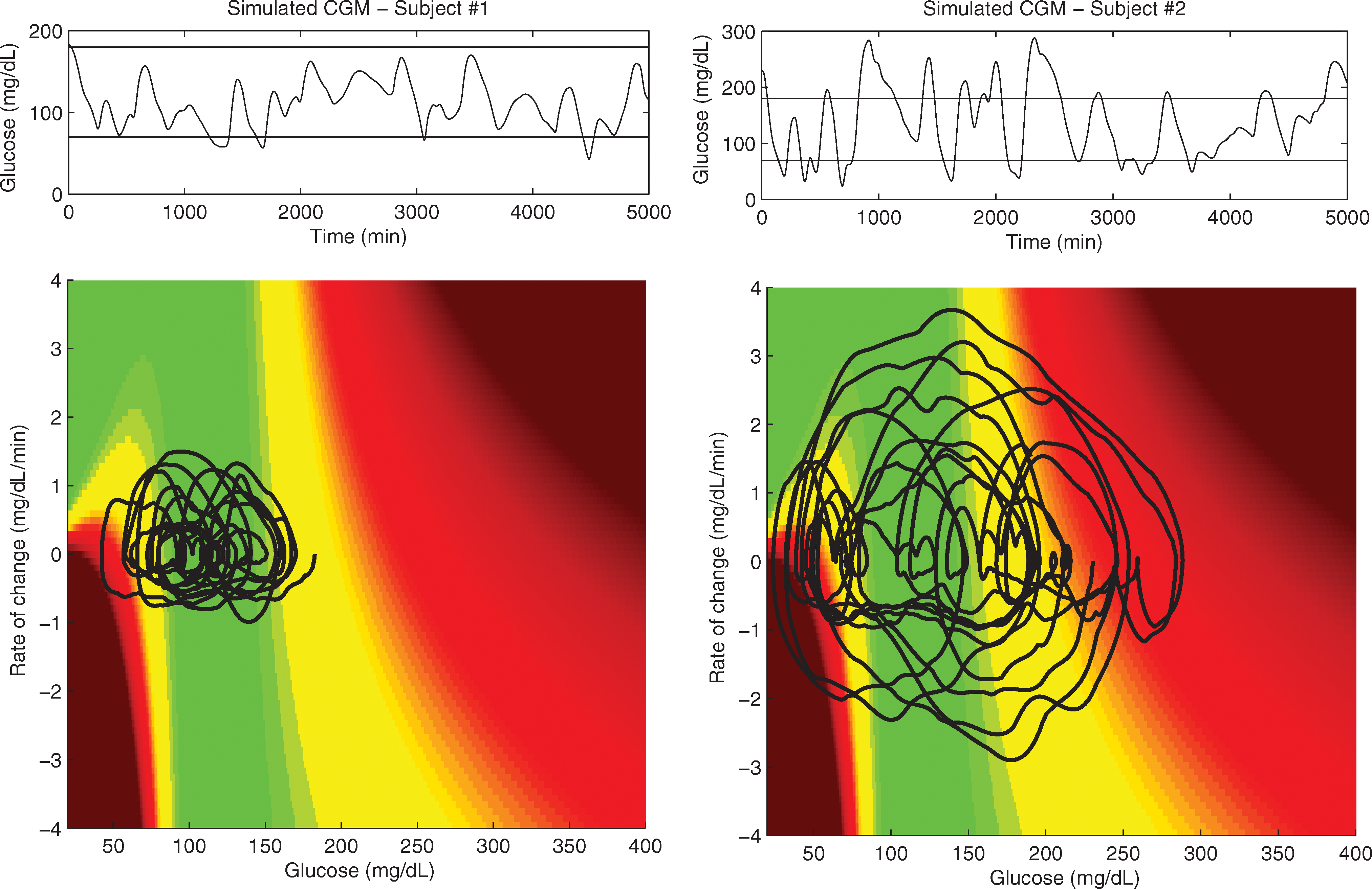
Glucose time-series (upper panels) and their trajectories (bottom panels) in the dynamic risk space for a well-controlled (left panel) and a badly controlled (right panel) subject. The greater area swept by the trajectory on the right could be used as an index of the poorer control of this subject with respect to the subject on the left. CGM, continuous glucose monitoring.

Finally, additional work will investigate further the structure of Eq. 8 or Eq. 4. In this work an exponential structure is considered for its simplicity as an amplifier in Eq. 8, but also other functions (e.g., tanh, atan) could be considered to achieve the same goal. Also, the information about the integral of risk could be embedded in a new definition of risk.

Footnotes

Acknowledgments

Prof. Boris Kovatchev (Department of Psychiatric Medicine, University of Virginia Health System, Charlottesville, VA) is acknowledged for having provided a portion of the FreeStyle Navigator™ data previously published.²⁵ Prof. Angelo Avogaro and Dr. Alberto Maran (Department of Clinical and Experimental Medicine, University of Padova, Padova, Italy) are acknowledged for the many useful discussions on the interpretation of CGM data that contributed to the development of this work.

Author Disclosure Statement

No competing financial interests exist.

References

Cobelli

, Dalla Man

, Sparacino

, Magni

, De Nicolao

, Kovatchev

. Diabetes: models, signals, and control. IEEE Reviews Biomed Eng, 2009; 2:54–96.

Rodbard

. Interpretation of continuous glucose monitoring data: glycemic variability and quality of glycemic control. Diabetes Technol Ther, 2009; 11:55–67.

Greven

, Beulens

JWJ

, Biesma

, Faiz

, de Valk

. Glycemic variability in inadequately controlled type 1 diabetes and type 2 diabetes on intensive insulin therapy: a cross-sectional, observational study. Diabetes Technol Ther, 2010; 12:695–699.

Hirsch

. Clinical review: realistic expectations and practical use of continuous glucose monitoring for the endocrinologist. J Clin Endocrinol Metab, 2009; 94:2232–2238.

Klonoff

. Continuous glucose monitoring: roadmap for 21st Century diabetes therapy. Diabetes Care, 2005; 28:1231–1239.

Ward

. The role of new technology in the early detection of hypoglycemia. Diabetes Technol Ther, 2004; 6:115–117.

Buckingham

. Clinical overview of continuous glucose monitoring. J Diabetes Sci Technol, 2008; 2:300–306.

Bequette

. Continuous glucose monitoring: real-time algorithms for calibration, filtering, and alarms. J Diabetes Sci Technol, 2010; 4:404–418.

Hovorka

. The future of continuous glucose monitoring: closed loop. Curr Diabetes Rev, 2008; 4:269–279.

10.

Rebrin

, Sheppard

, Steil

. Use of subcutaneous interstitial fluid glucose to estimate blood glucose: revisiting delay and sensor offset. J Diabetes Sci Technol, 2010; 4:1087–1098.

11.

Sparacino

, Facchinetti

, Cobelli

. “Smart” continuous glucose monitoring sensors: on-line signal processing issues. Sensors, 2010; 10:6751–6772.

12.

Kovatchev

, Cox

, Gonder-Frederick

, Clarke

. Symmetrization of the blood glucose measurement scale and its applications. Diabetes Care, 1997; 20:1655–1658.

13.

Hill

, Hindmarsh

, Stevens

, Stratton

, Levy

, Matthews

. A method for assessing quality of control from glucose profiles. Diabet Med, 2007; 24:753–758.

14.

Rodbard

. New and improved methods to characterize glycemic variability using continuous glucose monitoring. Diabetes Technol Ther, 2009; 11:551–565.

15.

Rodbard

. A semilogarithmic scale for glucose provides a balanced view of hyperglycemia and hypoglycemia. J Diabetes Sci Technol, 2009; 3:1395–1401.

16.

Kovatchev

, Cox

, Gonder-Frederick

, Young-Hyman

, Schlundt

, Clarke

. Assessment of risk for severe hypoglycaemia among adults with IDDM. Diabetes Care, 1998; 21:1870–1901.

17.

Kovatchev

, Straume

, Cox

, Fahry

. Risk analysis of blood glucose data: a quantitative approach to optimizing the control of insulin dependent diabetes. J Theoret Med, 2000; 3:1–10.

18.

Kovatchev

, Cox

, Kumar

, Gonder-Frederick

, Clarke

. Algorithmic evaluation of metabolic control and risk of severe hypoglycemia in type 1 and type 2 diabetes using self-monitoring blood glucose data. Diabetes Technol Ther, 2003; 5:817–828.

19.

Clarke

, Kovatchev

. Statistical tools to analyze continuous glucose monitor data. Diabetes Technol Ther, 2009; 11:45–54.

20.

Kovatchev

, Clarke

, Breton

, Brayman

, McCall

. Quantifying temporal glucose variability in diabetes via continuous glucose monitoring: mathematical methods and clinical application. Diabetes Technol Ther, 2005; 7:849–862.

21.

Cameron

, Bequette

, Wilson

, Buckingham

, Lee

, Niemeyer

. A closed-loop artificial pancreas based on risk management. J Diabetes Sci Technol, 2011; 5:368–379.

22.

Oppenheim

, Willsky

, Hamid

. Prentice Hall Signal Processing Series: Signals, Systems. Englewood Cliffs, NJ: Prentice Hall, 1997.

23.

De Nicolao

, Sparacino

, Cobelli

. Nonparametric input estimation in physiological systems: problems, methods and case studies. Automatica, 1997; 33:851–870.

24.

Palerm

, Bequette

. Hypoglycemia detection and prediction using continuous glucose monitoring: a study on hypoglycemic clamp data. J Diabetes Sci Technol, 2007; 1:624–629.

25.

Kovatchev

, Gonder-Frederick

, Cox

, Clarke

. Evaluating the accuracy of continuous glucose-monitoring sensors: continuous glucose-error grid analysis illustrated by TheraSense Freestyle Navigator data. Diabetes Care, 2004; 27:1922–1928.

26.

Rahaghi

, Gough

. Blood glucose dynamics. Diabetes Technol Ther, 2008; 10:81–94.