Hypoglycemic events in patients with type 1 diabetes (T1D) are associated with measurable electroencephalography (EEG) changes. Previous studies have, however, evaluated these changes on a single EEG channel level, whereas multivariate analysis of several EEG channels has been scarcely investigated. The aim of the present work is to use a coherence approach to quantitatively assess how hypoglycemia affects mutual connectivity of different brain areas.
Materials and Methods:
EEG multichannel data were obtained from 19 patients with T1D (58% males; mean age, 55 ± 2.4 years; diabetes duration, 28.5 ± 2.6 years; glycated hemoglobin, 8.0 ± 0.2%) who underwent a hyperinsulinemic–hypoglycemic clamp study. The information partial directed coherence (iPDC) function was computed through multivariate autoregressive models during eu- and hypoglycemia in the theta and alpha bands.
Results:
In passing from eu- to hypoglycemia, absolute values of the iPDC function tend to decrease in both bands in all combinations of the considered channels. In particular, the scalar indicator \documentclass{aastex}\usepackage{amsbsy}\usepackage{amsfonts}\usepackage{amssymb}\usepackage{bm}\usepackage{mathrsfs}\usepackage{pifont}\usepackage{stmaryrd}\usepackage{textcomp}\usepackage{portland, xspace}\usepackage{amsmath, amsxtra}\pagestyle{empty}\DeclareMathSizes{10}{9}{7}{6}\begin{document}$$\overline{\overline{\iota PDC}}$$ \end{document}, which summarizes iPDC information, significantly decreased (P < 0.01) in 17 of 19 subjects: from T5-A1A2 to C3-A1A2 from O1-A1A2 to C4-A1A2 and from O2-A1A2 to Cz-A1A2 in the theta band and from O1-A1A2 to T4-A1A2 and from O1-A1A2 to C4-A1A2 in the alpha band.
Conclusions:
The coherence decrease measured by iPDC in passing from eu- to hypoglycemia is likely related to the progressive loss of cognitive function and altered cerebral activity in hypoglycemia. This result encourages further quantitative investigation of EEG changes in hypoglycemia and of how EEG acquisition and real-time processing can support hypoglycemia alert systems.
Background
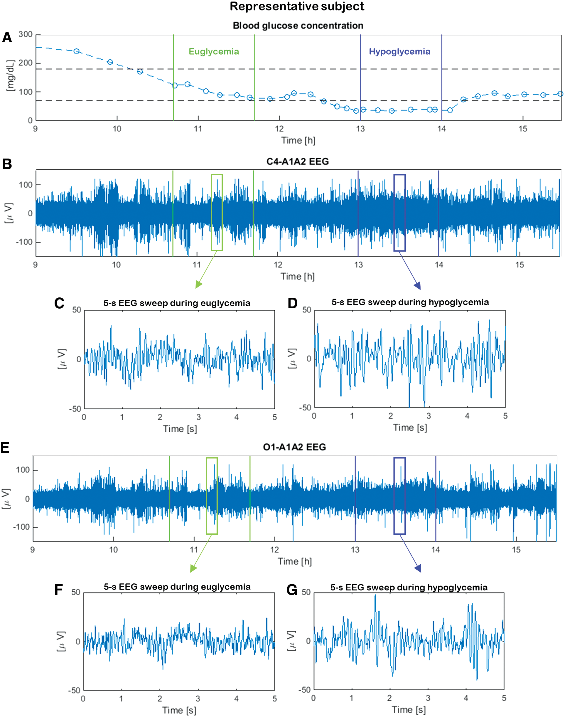
The first studies investigating the relationship between hypoglycemia and the electroencephalography (EEG) signal date back to the 1950s.1,2 Since then, several studies (e.g., Pramming et al.,3 Tribl et al.,4 and Hyllienmark et al.5) have proven that a power increase in the low-frequency EEG bands (i.e., higher amplitude of low-frequency EEG rhythms) takes place during hypoglycemia. These hypoglycemia-associated changes are independent of hypoglycemia awareness status in patients with type 1 diabetes (T1D).6 In particular, EEG power spectral density in the conventional theta (4–8 Hz) and alpha (8–13 Hz) bands increases during hypoglycemia with respect to euglycemia, confirming the higher amplitude of low-frequency EEG rhythms in hypoglycemia.7 Additionally, hypoglycemia also shows a decrease of EEG complexity.8 These changes in EEG signals can be qualitatively appreciated by visual inspection of the representative data in Figure 1, in which segments 5 s in duration (“sweeps”) measured in euglycemia are shown with those recorded in the same subject when he or she is exposed to hypoglycemia. At the single-channel level EEG in hypoglycemia (Fig. 1D and G) shows higher amplitudes in the low-frequency bands and greater regularity than the one in euglycemia (Fig. 1C and F). Based on this evidence, research prototype portable devices, able to measure the EEG signal by subcutaneous electrodes (with potential lifetime greater than 10 years) and analyze and classify it in real time, have been recently developed to investigate their usefulness in detecting hypoglycemia events.
Data from a representative subject during the hyperinsulinemic-hypoglycemic clamp: (A) blood glucose concentration (open circles denote reference YSI samples; the dashed lines denote their spline interpolation) and simultaneous (B) C4-A1A2 and (E) O1-A1A2 electroencephalography (EEG) recordings. Vertical green and blue lines refer to 1-h eu- and hypoglycemic intervals, respectively. For each glycemic condition, 5-s EEG sweeps are shown (C and D) for C4-A1A2 and (F and G) for O1-A1A2, where t = 0 is the sweep start time. (Color graphics available at www.liebertonline.com/dia)
Although the notion that hypoglycemia affects EEG rhythms is well established, limited information is available on if and how hypoglycemia influences the connectivity between different brain areas. To the best of our knowledge, existing publications have focused on univariate EEG studies. In the present study, we use a multivariate approach called information partial directed coherence (iPDC) to quantify the synchronization between EEG channel-pairs in eu- and hypoglycemic conditions. In particular, iPDC is computed through the use of multivariate autoregressive (MAR) models of T3-A1A2, T4-A1A2, T5-A1A2, T6-A1A2, P3-A1A2, P4-A1A2, Pz-A1A2, C3-A1A2, C4-A1A2, Cz-A1A2, O1-A1A2, and O2-A1A2 EEG channels recordings in 19 hospitalized T1D subjects enrolled in an insulin-induced experiment. The value of coherence in both the theta and alpha bands was examined when passing from eu- to hypoglycemia.
Materials and Methods
Experimental protocol and database
The database is taken by a study approved by the local ethical committee, and data from this study have previously been published by Sejling et al.6 and Fabris et al.8 In particular, 19 patients with T1D participated in this study. Inclusion and exclusion criteria have previously been described by Sejling et al.6 The diabetes patients underwent a hyperinsulinemic–hypoglycemic clamp with a target of 2.0–2.5 mmol/L. Hypoglycemia was induced by an intravenous infusion of fast-acting recombinant human insulin (Actrapid®; Novo Nordisk, Bagsvaerd, Denmark). The insulin was administered intravenously at an infusion rate of 1 mU/kg/min, and target blood glucose (BG) levels were obtained by a variable infusion of glucose (200 mg/mL). BG level was determined every 5 min by a laboratory analyzer (model YSI 2300; Yellow Springs Instrument Co., Yellow Springs, OH).
EEG recordings and glucose concentration samples were collected in parallel during the experiment. Participants were sitting in an armchair, not allowed to sleep, and under constant observation by a physician who evaluated signs of neuroglycopenia, while 19 EEG channels were recorded by a digital EEG recorder (model Easy II; Cadwell Laboratories, Kennewick, WA) using standard cap electrodes placed on the scalp according to the 10/20 international system. In particular, Fp1-A1A2, Fp2-A1A2, F7-A1A2, F8-A1A2, F3-A1A2, F4-A1A2, Fz-A1A2, T3-A1A2, T4-A1A2, T5-A1A2, T6-A1A2, C3-A1A2, C4-A1A2, Cz-A1A2, P3-A1A2, P4-A1A2, Pz-A1A2, O1-A1A2, and O2-A1A2 EEG channels were acquired. (Odd numbers represent the left hemisphere, and even numbers represent the right hemisphere. The capital letters F, T, C, P, and O identify the frontal, temporal, central parietal, and occipital lobes respectively.) The EEG scan was analogically low-pass-filtered at 70 Hz and then digitally acquired and sampled at 200 Hz. The dynamic range of the EEG was ±4,620 μV with an amplitude resolution of 0.14 μV. Internal noise level in the analog data acquisition system was estimated to be 1.3 μV root mean square. Figure 1 shows the BG data (Fig. 1A), as well as the C4-A1A2 and O1-A1A2 EEG recordings (Fig. 1B and E) collected in parallel in a representative subject during the daytime.
Pre-analysis
Only EEG channels in the temporal, central, parietal, and occipital lobes (i.e., the L = 12 EEG time-series referred to, respectively, as the T3-A1A2, T4-A1A2, T5-A1A2, T6-A1A2, P3-A1A2, P4-A1A2, Pz-A1A2, C3-A1A2, C4-A1A2, Cz-A1A2, O1-A1A2, and O2-A1A2 channels) were considered because their analysis is simplified from the virtual absence of artifacts (e.g., eye-induced, muscle activation-induced). EEG data were not band-pass-filtered before computing iPDC in order to avoid possible distortions in the results.9
A pre-analysis was developed considering, in each subject, two intervals referred to as eu- and hypoglycemia, respectively, targeted from the available BG data. In particular, for each subject, two 1-h intervals corresponding to eu- and hypoglycemia conditions, respectively, were identified from the BG time-series by visual inspection detecting when the glycemic thresholds at 70 and 180 mg/dL were crossed by a smoothing spline approximation of the samples (Fig. 1A). Representative randomly chosen 5-s EEG sweeps are also depicted to appreciate, albeit qualitatively, differences of the EEG signal in eu- (Fig. 1C and F) and hypoglycemia (Fig. 1D and G). Assessing the synchronization of pairs of EEG sweeps in the same glycemic condition by visual inspection is challenging, calling for the use of multivariate analysis tools.
iPDC definition
Coherence is a standard investigational tool in the multivariate analysis of biomedical signals, especially for EEG, and several definitions have been proposed.10,11 In particular, the iPDC has been recently presented by Takahashi et al.,12 as an improvement of partial directed coherence13 and general partial directed coherence.14 Indeed, iPDC is considered more stable than other approaches in coherence assessment when signals have large differences in their amplitudes, as happens with EEG in hypoglycemia compared with EEG in euglycemia in our case study.
Roughly speaking, iPDC is a multivariate spectral measure to compute the directed influences between any given pair of signals (i,j) of a multivariate dataset. This information is condensed in a complex function \documentclass{aastex}\usepackage{amsbsy}\usepackage{amsfonts}\usepackage{amssymb}\usepackage{bm}\usepackage{mathrsfs}\usepackage{pifont}\usepackage{stmaryrd}\usepackage{textcomp}\usepackage{portland, xspace}\usepackage{amsmath, amsxtra}\pagestyle{empty}\DeclareMathSizes{10}{9}{7}{6}\begin{document}$$iPDC_{i \leftarrow j} ( f )$$ \end{document} of the frequency f, which measures the relative interaction of the signal j with regard to signal i as compared with interactions of all js with other signals in the multivariate dataset. Although we refer the reader to Takahashi et al.12 for the mathematical details, the procedure for computing iPDC is briefly described by the following two steps.
In the first step, an MAR model is identified by fitting it against EEG data streams acquired from L different channels. Formally, letting x(n)\documentclass{aastex}\usepackage{amsbsy}\usepackage{amsfonts}\usepackage{amssymb}\usepackage{bm}\usepackage{mathrsfs}\usepackage{pifont}\usepackage{stmaryrd}\usepackage{textcomp}\usepackage{portland, xspace}\usepackage{amsmath, amsxtra}\pagestyle{empty}\DeclareMathSizes{10}{9}{7}{6}\begin{document}%\begin{align*}%{\textbf{\textit{x}} ( \textbf{\textit{n}} ) } = [%{\textbf{\textit{x_1}} ( \textbf{\textit{n}} ) ,%\textbf{\textit{x_2}} ( \textbf{\textit{n}} ) , \ldots ,%\textbf{\textit{x_L}} ( \textbf{\textit{n}} ) } ] ^T \ \ n = 1 , .%, N \tag{1}%\end{align*} \end{document}
(where T stands for transpose) be the vector containing the samples at the n-th sampling instant n (n = 1, …N) of the L considered EEG channels x1, x2, …, xL, the MAR model of order p is described as\documentclass{aastex}\usepackage{amsbsy}\usepackage{amsfonts}\usepackage{amssymb}\usepackage{bm}\usepackage{mathrsfs}\usepackage{pifont}\usepackage{stmaryrd}\usepackage{textcomp}\usepackage{portland, xspace}\usepackage{amsmath, amsxtra}\pagestyle{empty}\DeclareMathSizes{10}{9}{7}{6}\begin{document} \begin{align*}{\textbf{\textit{x}} ( \textbf{\textit{n}} ) } = - { \Sigma}_{r = 1}^p \textbf{\textit{A}}_\textbf{\textit{rx}} ( \textbf{\textit{n- r}} ) + \bi w ( \bi n ) \tag{2} \end{align*} \end{document}
where Ar (r = 1, …, p) are the L × L unknown matrices of model coefficients, and the L-size column vector w(n) is the innovation process with covariance matrix ΣW.12 The matrices Ar (r = 1, …, p) and ΣW are estimated by least squares exploiting the so-called Yule–Walker equations15:\documentclass{aastex}\usepackage{amsbsy}\usepackage{amsfonts}\usepackage{amssymb}\usepackage{bm}\usepackage{mathrsfs}\usepackage{pifont}\usepackage{stmaryrd}\usepackage{textcomp}\usepackage{portland, xspace}\usepackage{amsmath, amsxtra}\pagestyle{empty}\DeclareMathSizes{10}{9}{7}{6}\def\bi{\boldsymbol}\begin{document} \begin{align*} \begin{array}{ll} \left[ \begin{matrix} \textbf{\textit{R}}_{\textbf{\textit{{xx}}}} ( { \bf 0} ) \quad \textbf{\textit{R}}_{\textbf{\textit{{xx}}}} ( { \bf - 1} ) & \ldots & \textbf{\textit{R}}_{\textbf{\textit{{xx}}}} ( \textbf{\textit{- p + {\bf 1}}} ) \\ \textbf{\textit{R}}_{\textbf{\textit{{xx}}}} ( { \bf 1} ) \quad \textbf{\textit{R}}_{\textbf{\textit{{xx}}}} ( { \bf 0} ) & & \textbf{\textit{R}}_{\textbf{\textit{{xx}}}}( \textbf{\textit{- p + {\bf 2}}} ) \\ \vdots & \ddots & \vdots \\ \textbf{\textit{R}}_\textbf{\textit{{xx}}} ( \textbf{\textit{p}} -{\bf 1} ) \quad \textbf{\textit{R}}_\textbf{\textit{{xx}}} ( \textbf{\textit{p}} - {\bf 2} ) & \cdots & \textbf{\textit{R}}_{\textbf{\textit{{xx}}}} ( { \bf 0} ) \end{matrix} \right]&\left[ \begin{matrix} \textbf{\textit{A}}^{\textbf{\textit{T}}}_{\bf 1} \\ \textbf{\textit{A}}^{\textbf{\textit{T}}}_{\bf 2} \\ \vdots \\ \textbf{\textit{{A}}}^{\textbf{\textit{T}}}_{\textbf{\textit{p}}} \end{matrix} \right] \\ \quad= - \left[ \begin{matrix} \textbf{\textit{R}}_{\textbf{\textit{{xx}}}} ( { \bf 1} ) \\ \textbf{\textit{R}}_{\textbf{\textit{xx}}} ( { \bf 2} ) \\ \vdots \\ \textbf{\textit{R}}_{\textbf{\textit{xx}}} ( \textbf{\textit{p}} ) \end{matrix} \right]& \tag{3} \end{array} \end{align*} \end{document}
where the Rxx(k) matrices are the covariance matrices computed from the available EEG data as\documentclass{aastex}\usepackage{amsbsy}\usepackage{amsfonts}\usepackage{amssymb}\usepackage{bm}\usepackage{mathrsfs}\usepackage{pifont}\usepackage{stmaryrd}\usepackage{textcomp}\usepackage{portland, xspace}\usepackage{amsmath, amsxtra}\pagestyle{empty}\DeclareMathSizes{10}{9}{7}{6}\begin{document} \begin{align*} \textbf{\textit{R}}_{\textbf{\textit{{ xx } } }} ( \textbf { \textit { k } } ) = \begin{cases} \frac { 1 } { N } \Sigma_ { n = 0 }^{N - 1 - k } \textbf{\textit{ x } } ( \textbf{\textit { n } } ) \textbf{\textit{ x}}^{\textbf{\textit{T } }} ( \textbf{\textit { n + k} } ) \quad \quad \quad \quad \quad \quad k = 0 , 1 , . , N - 1 \\ \frac{1} { N } \Sigma_ { n = - k } ^ { N - 1 } \textbf{\textit{x} } ( \textbf{\textit{n}} ) \textbf{\textit{x}}^{\textbf{\textit{T} }} ( \textbf{\textit{n + k } } ) \ \ k = - ( N - 1 ) , - ( N - 2) , . , - 1 \end{cases}\tag{4} \end{align*} \end{document}
In Eq. 2 model order p is found by trials until the Akaike information criterion (AIC) index\documentclass{aastex}\usepackage{amsbsy}\usepackage{amsfonts}\usepackage{amssymb}\usepackage{bm}\usepackage{mathrsfs}\usepackage{pifont}\usepackage{stmaryrd}\usepackage{textcomp}\usepackage{portland, xspace}\usepackage{amsmath, amsxtra}\pagestyle{empty}\DeclareMathSizes{10}{9}{7}{6}\begin{document} \begin{align*}AIC ( p ) = Nln \mid { \boldsymbol{\Sigma}}_\textbf{\textit{W}} \mid + 2L^2 p \tag{5} \end{align*} \end{document}
(where | | denotes the matrix determinant) is minimized.16
In the second step, having defined the complex matrix B(f) as\documentclass{aastex}\usepackage{amsbsy}\usepackage{amsfonts}\usepackage{amssymb}\usepackage{bm}\usepackage{mathrsfs}\usepackage{pifont}\usepackage{stmaryrd}\usepackage{textcomp}\usepackage{portland, xspace}\usepackage{amsmath, amsxtra}\pagestyle{empty}\DeclareMathSizes{10}{9}{7}{6}\begin{document} \begin{align*} \textbf{\textit{B}} ( \textbf{\textit{f}} ) = \textbf{\textit{I}}_{\textbf{\textit{L}}} - \Sigma_{r = 1}^p \textbf{\textit{A}}_{\textbf{\textit{r}}} e^{ - j2 \pi f} \tag{6} \end{align*} \end{document}
where IL is the identity matrix and j is the imaginary unit in this equation, the iPDC complex function from the time-series j to the time-series i is obtained by\documentclass{aastex}\usepackage{amsbsy}\usepackage{amsfonts}\usepackage{amssymb}\usepackage{bm}\usepackage{mathrsfs}\usepackage{pifont}\usepackage{stmaryrd}\usepackage{textcomp}\usepackage{portland, xspace}\usepackage{amsmath, amsxtra}\pagestyle{empty}\DeclareMathSizes{10}{9}{7}{6}\begin{document} \begin{align*} iPDC_{i \leftarrow j} (f)= \sigma_{W_{ii}}^{-1/2} \frac{b_ij(f)}{\sqrt{\textbf{\textit{b}}_{\textbf{\textit{j}}}^{\textbf{\textit{H}}}( f){\boldsymbol{\Sigma}}_{\textbf{\textit{W}}}^{\textbf{\textit{- 1}}} \textbf{\textit{b}}_{\textbf{\textit{j}}} (f)}} \tag{7} \end{align*} \end{document}
where bj(f) and bij(f) are, respectively, the j-th column and the (j,i)-th element of matrix B(f), \documentclass{aastex}\usepackage{amsbsy}\usepackage{amsfonts}\usepackage{amssymb}\usepackage{bm}\usepackage{mathrsfs}\usepackage{pifont}\usepackage{stmaryrd}\usepackage{textcomp}\usepackage{portland, xspace}\usepackage{amsmath, amsxtra}\pagestyle{empty}\DeclareMathSizes{10}{9}{7}{6}\begin{document}$$\sigma_{W_{ii}}$$ \end{document} is the (i,i)-th element of the innovation covariance matrix ΣW, and the apex H in \documentclass{aastex}\usepackage{amsbsy}\usepackage{amsfonts}\usepackage{amssymb}\usepackage{bm}\usepackage{mathrsfs}\usepackage{pifont}\usepackage{stmaryrd}\usepackage{textcomp}\usepackage{portland, xspace}\usepackage{amsmath, amsxtra}\pagestyle{empty}\DeclareMathSizes{10}{9}{7}{6}\begin{document}$$\textbf{\textit{b}}_{\textbf{\textit{j}}}^{\textbf{\textit H}}$$ \end{document} stands for the Hermitian transpose (i.e., obtained from bj by taking the transpose and then the complex conjugate of its components).
The complex function \documentclass{aastex}\usepackage{amsbsy}\usepackage{amsfonts}\usepackage{amssymb}\usepackage{bm}\usepackage{mathrsfs}\usepackage{pifont}\usepackage{stmaryrd}\usepackage{textcomp}\usepackage{portland, xspace}\usepackage{amsmath, amsxtra}\pagestyle{empty}\DeclareMathSizes{10}{9}{7}{6}\begin{document}$$iPDC_{i \leftarrow j} ( f )$$ \end{document} of Eq. 7 is usually analyzed in terms of its absolute value.12
iPDC computation
iPDC analysis was applied to the first 15 min of the eu- and hypoglycemia intervals. As previously described in the Pre-analysis section, L = 12 EEG channels were considered, and each 15-min interval of eu- and hypoglycemia was divided in 5-s sweeps, resulting in N = 1,000 samples per sweep, a quantity sufficient to obtain stable results in terms of coherence estimation according to Florin et al.9 At the same time, 5-s intervals are narrow enough to invoke pseudostationarity assumptions on EEG (e.g., as done by Abásolo et al.17). For each sweep, an MAR model as in Eq. 2 was identified. Regarding the model order p, we first considered, for each sweep, the value minimizing AIC(p) of Eq. 5 among candidate orders ranging from 1 to 20; then, among the estimated values of p, we chose the highest and used it as the model order for all sweeps under analysis for a given subject (the resulting p was always 9 or 10). The rationale behind this decision is that, to detect coupling directions in multivariate oscillatory systems, the MAR model should have a high order,18 and at the same time, overestimating the model order is better than underestimating it.9 Then, for any pair (i,j), the function \documentclass{aastex}\usepackage{amsbsy}\usepackage{amsfonts}\usepackage{amssymb}\usepackage{bm}\usepackage{mathrsfs}\usepackage{pifont}\usepackage{stmaryrd}\usepackage{textcomp}\usepackage{portland, xspace}\usepackage{amsmath, amsxtra}\pagestyle{empty}\DeclareMathSizes{10}{9}{7}{6}\begin{document}$$iPDC_{i \leftarrow j} ( f )$$ \end{document} of Eq. 7 was computed in theta ([4–8] Hz) and alpha ([8–13] Hz) bands for each sweep. Eventually, the absolute mean profiles \documentclass{aastex}\usepackage{amsbsy}\usepackage{amsfonts}\usepackage{amssymb}\usepackage{bm}\usepackage{mathrsfs}\usepackage{pifont}\usepackage{stmaryrd}\usepackage{textcomp}\usepackage{portland, xspace}\usepackage{amsmath, amsxtra}\pagestyle{empty}\DeclareMathSizes{10}{9}{7}{6}\begin{document}$${\overline{PDC}}_{i \leftarrow j} ( f )$$ \end{document}, referred to the whole interval of 15 min, were computed by averaging the absolute values of the \documentclass{aastex}\usepackage{amsbsy}\usepackage{amsfonts}\usepackage{amssymb}\usepackage{bm}\usepackage{mathrsfs}\usepackage{pifont}\usepackage{stmaryrd}\usepackage{textcomp}\usepackage{portland, xspace}\usepackage{amsmath, amsxtra}\pagestyle{empty}\DeclareMathSizes{10}{9}{7}{6}\begin{document}$$iPDC_{i \leftarrow j} ( f )$$ \end{document} profiles estimated in the 5-s sweeps (throughout this article, for sake of brevity, the symbol \documentclass{aastex}\usepackage{amsbsy}\usepackage{amsfonts}\usepackage{amssymb}\usepackage{bm}\usepackage{mathrsfs}\usepackage{pifont}\usepackage{stmaryrd}\usepackage{textcomp}\usepackage{portland, xspace}\usepackage{amsmath, amsxtra}\pagestyle{empty}\DeclareMathSizes{10}{9}{7}{6}\begin{document}$${\overline{{PDC}}}$$ \end{document} will be used without explicitly showing the dependence on frequency and channel pair).
iPDC values analysis
Because the values of \documentclass{aastex}\usepackage{amsbsy}\usepackage{amsfonts}\usepackage{amssymb}\usepackage{bm}\usepackage{mathrsfs}\usepackage{pifont}\usepackage{stmaryrd}\usepackage{textcomp}\usepackage{portland, xspace}\usepackage{amsmath, amsxtra}\pagestyle{empty}\DeclareMathSizes{10}{9}{7}{6}\begin{document}$${ \overline {{PDC}}}$$ \end{document} can be pretty low, it is necessary, before evaluating changes passing from eu- to hypoglycemia, to determine an analytical threshold exploiting surrogate data. In particular, 15-min surrogate data in eu- and hypoglycemia were obtained randomly changing the time order of a set of real data (i.e., randomly permuting in temporal order the samples of the original series and so maintaining mean, variance, and histogram distribution of the original data).19 Then, as for real data, iPDC was estimated, and two thresholds for eu- and hypoglycemia, respectively, were calculated as 5% of the absolute value of \documentclass{aastex}\usepackage{amsbsy}\usepackage{amsfonts}\usepackage{amssymb}\usepackage{bm}\usepackage{mathrsfs}\usepackage{pifont}\usepackage{stmaryrd}\usepackage{textcomp}\usepackage{portland, xspace}\usepackage{amsmath, amsxtra}\pagestyle{empty}\DeclareMathSizes{10}{9}{7}{6}\begin{document}$${ \overline {{PDC}}}$$ \end{document}.20 Thus, before applying the statistical tests to evaluate if there were remarkable changes passing from eu- to hypoglycemia, it was checked if \documentclass{aastex}\usepackage{amsbsy}\usepackage{amsfonts}\usepackage{amssymb}\usepackage{bm}\usepackage{mathrsfs}\usepackage{pifont}\usepackage{stmaryrd}\usepackage{textcomp}\usepackage{portland, xspace}\usepackage{amsmath, amsxtra}\pagestyle{empty}\DeclareMathSizes{10}{9}{7}{6}\begin{document}$${ \overline {{PDC}}}$$ \end{document} results were above the threshold estimated at any frequency. Eventually, to assess for each subject whether or not the changes in the absolute value of \documentclass{aastex}\usepackage{amsbsy}\usepackage{amsfonts}\usepackage{amssymb}\usepackage{bm}\usepackage{mathrsfs}\usepackage{pifont}\usepackage{stmaryrd}\usepackage{textcomp}\usepackage{portland, xspace}\usepackage{amsmath, amsxtra}\pagestyle{empty}\DeclareMathSizes{10}{9}{7}{6}\begin{document}$${\overline{PDC}}$$ \end{document} were statistically significant when passing from eu- to hypoglycemia, paired Student's t tests were computed under the hypothesis of normal distribution of samples (Lilliefors test); otherwise, Wilcoxon rank-sign tests were considered (a value of P < 0.05 was considered significant). After that, for each subject, the average value of \documentclass{aastex}\usepackage{amsbsy}\usepackage{amsfonts}\usepackage{amssymb}\usepackage{bm}\usepackage{mathrsfs}\usepackage{pifont}\usepackage{stmaryrd}\usepackage{textcomp}\usepackage{portland, xspace}\usepackage{amsmath, amsxtra}\pagestyle{empty}\DeclareMathSizes{10}{9}{7}{6}\begin{document}$${\overline{PDC}}$$ \end{document} was computed to obtain a scalar indicator for the eu- and hypoglycemia interval. This scalar indicator (which subsequently in this article will be denoted by the symbol \documentclass{aastex}\usepackage{amsbsy}\usepackage{amsfonts}\usepackage{amssymb}\usepackage{bm}\usepackage{mathrsfs}\usepackage{pifont}\usepackage{stmaryrd}\usepackage{textcomp}\usepackage{portland, xspace}\usepackage{amsmath, amsxtra}\pagestyle{empty}\DeclareMathSizes{10}{9}{7}{6}\begin{document}$${\overline{\overline {{{PDC}}}}}$$ \end{document}) is obviously much simpler to handle than the function \documentclass{aastex}\usepackage{amsbsy}\usepackage{amsfonts}\usepackage{amssymb}\usepackage{bm}\usepackage{mathrsfs}\usepackage{pifont}\usepackage{stmaryrd}\usepackage{textcomp}\usepackage{portland, xspace}\usepackage{amsmath, amsxtra}\pagestyle{empty}\DeclareMathSizes{10}{9}{7}{6}\begin{document}$${ \overline{PDC}}$$ \end{document} for the analysis.
Results
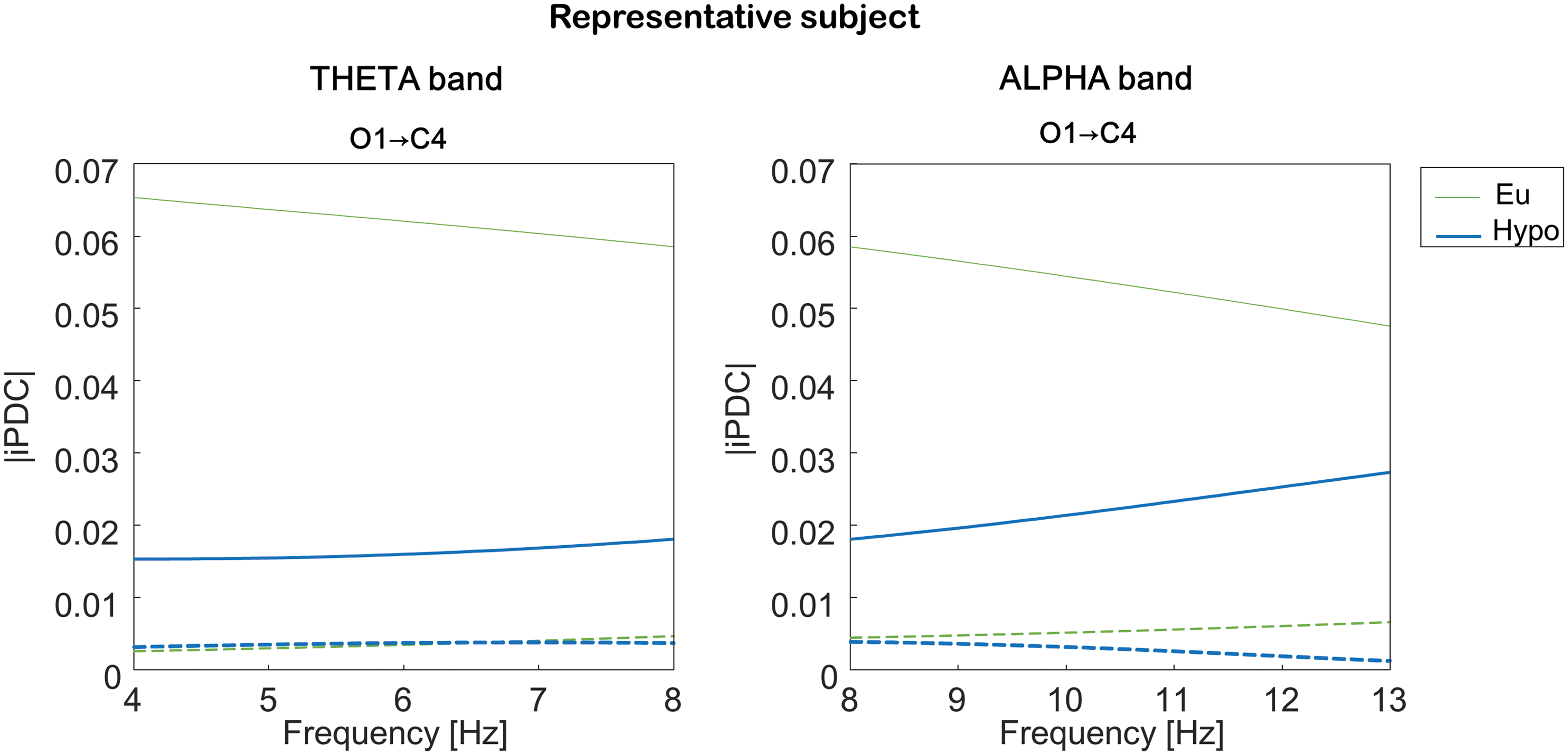
The absolute values of the iPDC function \documentclass{aastex}\usepackage{amsbsy}\usepackage{amsfonts}\usepackage{amssymb}\usepackage{bm}\usepackage{mathrsfs}\usepackage{pifont}\usepackage{stmaryrd}\usepackage{textcomp}\usepackage{portland, xspace}\usepackage{amsmath, amsxtra}\pagestyle{empty}\DeclareMathSizes{10}{9}{7}{6}\begin{document}$$iPDC_{i \leftarrow j} ( f )$$ \end{document} computed in two 5-s representative sweeps are shown in Figure 2 for a representative participant in both the theta (Fig. 2, left panel) and alpha (Fig. 2, right panel) bands before (thin upper line) and after entering in hypoglycemia (thick lower line). The absolute values of iPDC are rather low but above the computed thresholds (dashed lines) that indicate the minimal level of iPDC considered as null. Remarkably, a very visible change passing from eu- to hypoglycemia can be observed in both bands. All the other sweeps referred to this participant showed iPDC profiles for all combinations of channels qualitatively similar to those of Figure 2. The same, on average, happens in the entire database of subjects.
Information partial directed coherence (iPDC) in a representative subject. The absolute value of iPDC from O1-A1A2 to C4-A1A2 was computed from a randomly chosen 5-s sweep in the (left panel) theta and (right panel) alpha bands in eu- (thin upper line) and hypoglycemia (thick lower line). The dashed lines stand for the iPDC threshold computed from surrogate data. (Color graphics available at www.liebertonline.com/dia)
Considering the function \documentclass{aastex}\usepackage{amsbsy}\usepackage{amsfonts}\usepackage{amssymb}\usepackage{bm}\usepackage{mathrsfs}\usepackage{pifont}\usepackage{stmaryrd}\usepackage{textcomp}\usepackage{portland, xspace}\usepackage{amsmath, amsxtra}\pagestyle{empty}\DeclareMathSizes{10}{9}{7}{6}\begin{document}$${ \overline{PDC}}$$ \end{document}, it tends to decrease when passing from eu- to hypoglycemia in both theta and alpha bands in all combinations of the considered EEG channels. An example of results is documented in Figure 3, which displays, for the representative subject, \documentclass{aastex}\usepackage{amsbsy}\usepackage{amsfonts}\usepackage{amssymb}\usepackage{bm}\usepackage{mathrsfs}\usepackage{pifont}\usepackage{stmaryrd}\usepackage{textcomp}\usepackage{portland, xspace}\usepackage{amsmath, amsxtra}\pagestyle{empty}\DeclareMathSizes{10}{9}{7}{6}\begin{document}$${ \overline{PDC}}$$ \end{document} from T5-A1A2 to C3-A1A2 and from O1-A1A2 to C4-A1A2 in the theta band (Fig. 3, left panels) and from O1-A1A2 to T4-A1A2 and from O1-A1A2 to C4-A1A2 in the alpha band (Fig. 3, right panels) in eu- (thin upper line) and hypoglycemia (thick lower line). Considering the entire dataset, in the theta band the function \documentclass{aastex}\usepackage{amsbsy}\usepackage{amsfonts}\usepackage{amssymb}\usepackage{bm}\usepackage{mathrsfs}\usepackage{pifont}\usepackage{stmaryrd}\usepackage{textcomp}\usepackage{portland, xspace}\usepackage{amsmath, amsxtra}\pagestyle{empty}\DeclareMathSizes{10}{9}{7}{6}\begin{document}$${ \overline{PDC}}$$ \end{document} significantly decreases (P < 0.01) in 17 of 19 subjects from T5-A1A2 to C3-A1A2, from O1-A1A2 to C4-A1A2, and from O2-A1A2 to Cz-A1A2. In the alpha band it significantly decreases (P < 0.01) in 17 of 19 subjects from O1-A1A2 to T4-A1A2 and from O1-A1A2 to C4-A1A2.
The information partial directed coherence function (\documentclass{aastex}\usepackage{amsbsy}\usepackage{amsfonts}\usepackage{amssymb}\usepackage{bm}\usepackage{mathrsfs}\usepackage{pifont}\usepackage{stmaryrd}\usepackage{textcomp}\usepackage{portland, xspace}\usepackage{amsmath, amsxtra}\pagestyle{empty}\DeclareMathSizes{10}{9}{7}{6}\begin{document}$${ \overline {iPDC}}$$ \end{document}) in a representative subject. The \documentclass{aastex}\usepackage{amsbsy}\usepackage{amsfonts}\usepackage{amssymb}\usepackage{bm}\usepackage{mathrsfs}\usepackage{pifont}\usepackage{stmaryrd}\usepackage{textcomp}\usepackage{portland, xspace}\usepackage{amsmath, amsxtra}\pagestyle{empty}\DeclareMathSizes{10}{9}{7}{6}\begin{document}$${ \overline {iPDC}}$$ \end{document} is estimated (left panels) from T5-A1A2 to C3-A1A2 and from O1-A1A2 to C4-A1A2 in the theta band and (right panels) from O1-A1A2 to C4-A1A2 and from O1-A1A2 to T4-A1A2 in the alpha band in eu- (thin upper line) and hypo- (thick lower line) glycemia. (Color graphics available at www.liebertonline.com/dia)
In Figure 4 we report a box plot of the values, obtained from the entire pool of subjects, of the scalar indicator \documentclass{aastex}\usepackage{amsbsy}\usepackage{amsfonts}\usepackage{amssymb}\usepackage{bm}\usepackage{mathrsfs}\usepackage{pifont}\usepackage{stmaryrd}\usepackage{textcomp}\usepackage{portland, xspace}\usepackage{amsmath, amsxtra}\pagestyle{empty}\DeclareMathSizes{10}{9}{7}{6}\begin{document}$${ \overline{\overline{PDC}}}$$ \end{document} for the eu- and hypoglycemic intervals. In particular, \documentclass{aastex}\usepackage{amsbsy}\usepackage{amsfonts}\usepackage{amssymb}\usepackage{bm}\usepackage{mathrsfs}\usepackage{pifont}\usepackage{stmaryrd}\usepackage{textcomp}\usepackage{portland, xspace}\usepackage{amsmath, amsxtra}\pagestyle{empty}\DeclareMathSizes{10}{9}{7}{6}\begin{document}$${ \overline{\overline{PDC}}}$$ \end{document} from O1-A1A2 to C4-A1A2 tends to decrease (P < 0.01) passing from eu- to hypoglycemia, and its variability tends to decrease passing from eu- to hypoglycemia.
The scalar indicator of the information partial directed coherence function (\documentclass{aastex}\usepackage{amsbsy}\usepackage{amsfonts}\usepackage{amssymb}\usepackage{bm}\usepackage{mathrsfs}\usepackage{pifont}\usepackage{stmaryrd}\usepackage{textcomp}\usepackage{portland, xspace}\usepackage{amsmath, amsxtra}\pagestyle{empty}\DeclareMathSizes{10}{9}{7}{6}\begin{document}$${\overline{\overline{PDC}}}$$ \end{document}) from the entire pool of subjects (n = 19). Box plots are shown of \documentclass{aastex}\usepackage{amsbsy}\usepackage{amsfonts}\usepackage{amssymb}\usepackage{bm}\usepackage{mathrsfs}\usepackage{pifont}\usepackage{stmaryrd}\usepackage{textcomp}\usepackage{portland, xspace}\usepackage{amsmath, amsxtra}\pagestyle{empty}\DeclareMathSizes{10}{9}{7}{6}\begin{document}$${\overline{\overline{PDC}}}$$ \end{document} from O1-A1A2 to C4-A1A2 in eu- and hypoglycemia in (left panel) theta and (right panel) alpha bands from all subjects. In each box the central line is the median value, the edges of the box are the 75th and 25th percentiles, the whiskers extend to the most extreme data points that are not outliers, and the crosses plotted individually stand for the outliers. (Color graphics available at www.liebertonline.com/dia)
Because of \documentclass{aastex}\usepackage{amsbsy}\usepackage{amsfonts}\usepackage{amssymb}\usepackage{bm}\usepackage{mathrsfs}\usepackage{pifont}\usepackage{stmaryrd}\usepackage{textcomp}\usepackage{portland, xspace}\usepackage{amsmath, amsxtra}\pagestyle{empty}\DeclareMathSizes{10}{9}{7}{6}\begin{document}$${\overline{\overline{PDC}}}$$ \end{document} changes in hypoglycemia, it is interesting to assess, albeit in a preliminary fashion, the potential discriminatory power of a classifier driven by \documentclass{aastex}\usepackage{amsbsy}\usepackage{amsfonts}\usepackage{amssymb}\usepackage{bm}\usepackage{mathrsfs}\usepackage{pifont}\usepackage{stmaryrd}\usepackage{textcomp}\usepackage{portland, xspace}\usepackage{amsmath, amsxtra}\pagestyle{empty}\DeclareMathSizes{10}{9}{7}{6}\begin{document}$${\overline{\overline{PDC}}}$$ \end{document}. To do so, we exploited \documentclass{aastex}\usepackage{amsbsy}\usepackage{amsfonts}\usepackage{amssymb}\usepackage{bm}\usepackage{mathrsfs}\usepackage{pifont}\usepackage{stmaryrd}\usepackage{textcomp}\usepackage{portland, xspace}\usepackage{amsmath, amsxtra}\pagestyle{empty}\DeclareMathSizes{10}{9}{7}{6}\begin{document}$${\overline{\overline{PDC}}}$$ \end{document} from O1-A1A2 to C4-A1A2 related to the 17 subjects in whom coherence significantly decreased passing from eu- to hypoglycemia. These values were used to train a support vector machine classifier (with a gaussian radial basis function kernel with a scaling factor of 1.108). In particular, using the leaving-one-out approach, 16 out of 17 observations were used as the validation set, and the remaining observation was used as the training set (each observation includes \documentclass{aastex}\usepackage{amsbsy}\usepackage{amsfonts}\usepackage{amssymb}\usepackage{bm}\usepackage{mathrsfs}\usepackage{pifont}\usepackage{stmaryrd}\usepackage{textcomp}\usepackage{portland, xspace}\usepackage{amsmath, amsxtra}\pagestyle{empty}\DeclareMathSizes{10}{9}{7}{6}\begin{document}$${\overline{\overline{PDC}}}$$ \end{document} in both the theta and alpha bands for each subject). This step is repeated on all ways to cut the original sample.
Classification resulted in 12 of 17 euglycemic events (true-negative rate) and in 13 of 17 hypoglycemic events (true-positive rate) correctly estimated, corresponding to a specificity of 71%, a sensitivity of 76%, and an accuracy of 74%. These classification results are in line, if not slightly better, than those reported in previous EEG studies in hypoglycemia.21,22 Iaione and Marques22 reported an overall accuracy rate of 71.3%, sensitivity of 71.1%, and specificity of 71.5% in seven subjects during euglycemia and spontaneous hypoglycemia, and Nguyen et al.21 showed a sensitivity and specificity of 75% and 60%, respectively, in five T1D patients during an overnight clamp.
The classification performance from \documentclass{aastex}\usepackage{amsbsy}\usepackage{amsfonts}\usepackage{amssymb}\usepackage{bm}\usepackage{mathrsfs}\usepackage{pifont}\usepackage{stmaryrd}\usepackage{textcomp}\usepackage{portland, xspace}\usepackage{amsmath, amsxtra}\pagestyle{empty}\DeclareMathSizes{10}{9}{7}{6}\begin{document}$${\overline{\overline{PDC}}}$$ \end{document} resulted in a sensitivity and specificity higher than those obtained by us, on the same database, by applying univariate analysis exploiting the integral of the power spectral density, the integral of the logarithm of the squared power spectral density, the centroid frequency,23 and the reactivity index.24 Both sensitivity and specificity in the hypodetection did not exceed 63%.
Discussion
Since the first studies investigating the relationship between hypoglycemia and the EEG signal, several works have proven that a power increase in the low-frequency bands takes place during hypoglycemia. However, multivariate analysis considering more EEG channels simultaneously has been poorly investigated. In this work, in 19 T1D subjects enrolled in an insulin-induced hypoglycemia experiment, a subset of 12 EEG channels was analyzed by the computation of iPDC (i.e., a function that measures the synchronization between two signals in a multivariate dataset). Our results show that EEG coherence is affected by hypoglycemia in both the theta and alpha bands. In particular, the absolute iPDC mean values \documentclass{aastex}\usepackage{amsbsy}\usepackage{amsfonts}\usepackage{amssymb}\usepackage{bm}\usepackage{mathrsfs}\usepackage{pifont}\usepackage{stmaryrd}\usepackage{textcomp}\usepackage{portland, xspace}\usepackage{amsmath, amsxtra}\pagestyle{empty}\DeclareMathSizes{10}{9}{7}{6}\begin{document}$${ \overline{PDC}}$$ \end{document} significantly decreased (P < 0.01) passing from eu- to hypoglycemia in 17 of 19 subjects: from T5-A1A2 to C3-A1A2, from O1-A1A2 to C4-A1A2, and from O2-A1A2 to Cz-A1A2 in the theta band and from O1-A1A2 to T4-A1A2 and from O1-A1A2 to C4-A1A2 in the alpha band. This coherence drop suggests that hypoglycemia not only results in an increase of low-frequency power bands as shown in the literature, but also in a decrease in the EEG coherence, most likely related to the progressive loss of cognitive function and altered cerebral activity. Therefore, the methods and results of the present article can represent a useful contribution for a subsequent neurophysiologically based analysis of the effect of hypoglycemia on brain connectivity, in line with the complexity of hypoglycemia-associated cognitive decline.25
From a methodological point of view, our work shows that, in addition to EEG indicators obtained at the single-channel level, those computed from multivariate EEG analysis change in passing from eu- to hypoglycemia. Previous reports suggested that this kind of changes could be even used to investigate the possible use of the brain as a biosensor to detect hypoglycemia in T1D through EEG monitoring by subcutaneous electrodes (with a potential lifetime of several years) and real-time data processing by means of a multiparameter algorithm.26,27 With regard to this aspect, the accuracy achieved in this study may seem far from ideal, but a further investigation of the potential usefulness of EEG in detecting hypoglycemia is still warranted. The benefit of EEG as a biomarker is that the hypoglycemia-associated EEG changes are not blunted during hypoglycemia in patients with hypoglycemia unawareness, in contrast to the symptom of hypoglycemia, the counterregulatory hormonal response, and skin temperature changes.25,28 An EEG-based hypoglycemia detection device, however, still needs to be tested in a clinical setting. Certainly, fundamental issues, such as sensitivity, specificity, reliability, resolution, and influence of activity, must be carefully addressed before demonstrating a real-time usability of such a device.
Future developments of the present work will relate to the neurophysiological interpretation of the results, the complementarity of iPDC with methods already studied for EEG assessment in hypoglycemia, and a more sophisticated investigation of per-subject classifiers for hypoglycemia detection using different combinations of EEG indicators.
Footnotes
Author Disclosure Statement
No competing financial interests exist.
References
1.
ReganPF3rd, Browne-MayersAN: Electroencephalography, frequency analysis and consciousness; a correlation during insulin-induced hypoglycemia. J Nerv Ment Dis, 1956; 124:142–147.
PrammingS, ThorsteinssonB, BendtsonI, et al.: The relationship between symptomatic and biomechanical hypoglycemia in insulin-dependent diabetic patients. J Intern Med, 1990; 228:641–646.
4.
TriblG, HoworkaK, HegerG, et al.: EEG topography during insulin-induced hypoglycemia in patients with insulin-dependent diabetes mellitus. Eur Neurol, 1996; 36:303–309.
5.
HyllienmarkL, MaltezJ, DandenellA, et al.: EEG abnormalities with and without relation to severe hypoglycaemia in adolescents with type 1 diabetes. Diabetologia, 2005; 48:412–419.
6.
SejlingAS, KjaerTW, Pedersen-BjergaardU, et al.: Hypoglycemia-associated changes in electroencephalogram in patients with type 1 diabetes and normal hypoglycemia awareness or unawareness. Diabetes, 2014; 64:1760–1769.
7.
LarsenA, HojlundK, PoulsenMK, et al.: Hypoglycemia-associated electroencephalogram and electrocardiogram changes appear simultaneously. J Diabetes Sci Technol, 2013; 7:93–99.
8.
FabrisC, SparacinoG, SejlingAS, et al.: Hypoglycemia-related EEG changes assessed by multiscale entropy. Diabetes Technol Ther, 2014; 16:688–694.
9.
FlorinE, GrossJ, PfeiferJ, et al.: Reliability of multivariate causality measures for neural data. J Neurosci Methods, 2011; 198:344–358.
10.
TakahashiDY, BaccalàLA, SameshimaK: Information partial directed coherence. In: Methods in Brain Connectivity Inference Through Multivariate Time Series Analysis. Boca Raton, FL: CRC Press, 2014:75–86.
11.
BlinowskaKJ: Review of the methods of determination of directed connectivity from multichannel data. Med Biol Eng Comput, 2011; 49:521–529.
BaccaláLA, SameshimaK: Partial directed coherence: a new concept in neural structure determination. Biol Cybern, 2001; 84:463–473.
14.
BaccaláLA, SameshimaK, TakahashiDY: Generalized partial directed coherence. In: Proceedings of the 15th International Conference on Digital Signal Processing. Piscataway, NJ: IEEE, 2007:163–166.
15.
KaySM: Modern Spectral Estimation. Englewood Cliffs, NJ: Prentice Hall, 1999.
16.
AkaikeH: Information theory and an extension of the maximum likelihood principle. In: Springer Series in Statistics: Selected Papers of Hirotugu Akaike. New York: Springer, 1998:199–213.
17.
AbásoloD, HorneroR, EspinoP, et al.: Analysis of regularity in the EEG background activity of Alzheimer's disease patients with approximate entropy. Clin Neurophysiol, 2005; 116:1826–1834.
18.
WinterhalderM, SchelterB, TimmerJ: Detecting coupling directions in multivariate oscillatory systems. Int J Bifurcation Chaos, 2007; 17:3735–3739.
19.
FaesL, PinnaGD, PortaA, et al.: Surrogate data analysis for assessing the significance of the coherence function. IEEE Trans Biomed Eng, 2004; 51:1156–1166.
20.
de BritoCS, BaccaláLA, TakahashiDY, et al.: Asymptotic behaviour of generalized partial directed coherence. Conf Proc IEEE Eng Med Biol Soc, 2010; 2010:1718–1721.
21.
NguyenLB, NguyenAV, LingSH, et al.: Combining genetic algorithm and Levenberg-Marquardt algorithm in training neural network for hypoglycemia detection using EEG signals. Conf Proc IEEE Eng Med Biol Soc, 2013; 2013:5386–5389.
22.
IaioneF, MarquesJL: Methodology for hypoglycaemia detection based on the processing, analysis and classification of the electroencephalogram. Med Biol Eng Comput, 2005; 43:501–507.
23.
RemvigLS, ElsborgR, SejlingAS, et al.: Hypoglycemia-related electroencephalogram changes are independent of gender, age, duration of diabetes, and awareness status in type 1 diabetes. J Diabetes Sci Technol, 2012; 6:1337–1344.
24.
GoljahaniA, D'AvanzoC, SchiffS, et al.: A novel method for the determination of the EEG individual alpha frequency. Neuroimage, 2012; 60:774–786.
25.
CryerPE: Symptoms of hypoglycemia, thresholds for their occurrence, and hypoglycemia unawareness. Endocrinol Metab Clin North Am, 1999; 28:495–500.
26.
ElsborgR, RemvigLS, Beck-NielsenH, et al.: Detecting hypoglycemia by using the brain as a biosensor. In: Biosensors for Health, Environment and Biosecurity. Rijeka, Croatia: InTech, 2011:273–292.
27.
JuhlCB, HojlundK, ElsborgR, et al.: Automated detection of hypoglycemia-induced EEG changes recorded by subcutaneous electrodes in subjects with type 1 diabetes—the brain as a biosensor. Diabetes Res Clin Pract, 2010; 88:22–28.
28.
CryerPE: Mechanisms of hypoglycemia-associated autonomic failure in diabetes. N Engl J Med, 2013; 369:362–372.