Predicting Insulin Treatment Scenarios with the Net Effect Method: Domain of Validity

Abstract

Background:

A simulation methodology based on the net effect, a signal estimated from continuous glucose monitoring (CGM) and insulin data accounting for sources of glucose variability, for example, meals and exercise, has been proposed. This method has been recently used to “replay” real-life treatment scenarios and determine the minimal level of CGM sensor accuracy required for nonadjunctive use. Given the potential of the net effect method, it is important to assess its domain of validity.

Methods:

The UVA/Padova type 1 diabetes simulator is used to generate glucose and insulin data. The net effect signal is estimated and used to predict the glucose profiles resulting from the following therapy modifications: (1) basal insulin increase/decrease, (2) bolus reduction to prevent hypoglycemia, (3) bolus addition after CGM hyperalarms, (4) hypotreatment addition after CGM hypoalarms. Results of the net effect method are compared with the reference provided by the UVA/Padova simulator.

Results:

The net effect method (1) well predicts the effect of small basal insulin adjustments (±10%), but overestimates time in hypo/hyperglycemia for larger adjustments (±50%); (2) underestimates the bolus reduction required to prevent hypoglycemia; (3) underestimates time in hyperglycemia when introducing correction boluses; and (4) overestimates time in hypoglycemia when introducing hypotreatments.

Conclusions:

The net effect method is reliable for small adjustments of basal insulin, while outside this domain of validity it can provide inaccurate results.

Introduction

Mathematical models of type 1 diabetes (T1D) patient physiology are powerful tools that can be used to test in silico new insulin therapies, including those based on sensors for continuous glucose monitoring (CGM).¹ The UVA/Padova T1D simulator, for example, accepted by FDA in 2008 as a substitute to preclinical trials for certain insulin treatments² was shown, in its 2013 release,³ to be able to reproduce the main glycemic outcomes observed in clinical trials.⁴ A circadian model of insulin sensitivity was recently developed by our group,⁵ thus extending the use of the simulator from a single meal to multiple days. Other simulation models for in silico assessment of closed-loop control algorithms were proposed in Hovorka et al.,⁶ Wilinska et al.,⁷ and Kanderian et al.⁸

Recently, a different modeling methodology to run in silico experiments was proposed by Patek et al.⁹ The method is schematized in Figure 1. Given a model of T1D patient physiology, CGM and insulin pump data simultaneously recorded in a T1D patient in a certain time window are used to retrospectively estimate a signature of blood glucose (BG) variability, called net effect (Fig. 1, step A). This net effect signal is assumed to reflect a combination of components contributing to the patient's glucose variability in the specific time window studied, including meals, variation in insulin sensitivity, and exercise. The net effect signal estimated from the patient's data is then used as a forcing input to the patient model (Fig. 1, step B) to predict the effect of a modified insulin therapy on the patient's glucose concentration in the same time window where data for the net effect estimation were collected.

FIG. 1.

The steps of the net effect method. Step A (retrospective): the net effect signal is estimated from measured CGM data, insulin therapy, and a model of T1D patient physiology with known parameters. Step B (prospective): the net effect signal, estimated in step A, is used as forcing input of the T1D patient physiology model to predict glucose concentration in consequence of a given insulin therapy. CGM, continuous glucose monitoring.

The advantage of the net effect method is that it allows circumventing the necessity of mathematically describing sources of glucose variability, such as exercise, which are currently not incorporated in the most popular T1D simulators, including the UVA/Padova simulator.

The net effect method has been recently used by Kovatchev et al.¹⁰ to assess the minimal level of CGM sensor accuracy required for nonadjunctive use. A database of CGM and insulin time series, collected in 56 T1D subjects, was first used to estimate the net effect and, then, to predict the response to insulin therapies based on the nonadjunctive use of CGM, for example, by adding rescue carbohydrates and correction boluses according to CGM alarms, or modifying existing meal boluses according to the CGM trend. Based on these simulations, the authors concluded that the use of CGM for insulin dosing is feasible for sensors with a mean absolute relative difference (MARD) lower or equal than 10%.

This result was used in the work by Kovatchev¹¹ and Castle and Jacobs¹² to comment on the improved accuracy of the Dexcom G4 Platinum CGM sensor (Dexcom, Inc., San Diego, CA) with software 505.^13,14 However, the net effect method was originally proposed by Patek et al.⁹ for designing basal insulin adjustments, and thus, it is important to evaluate the reliability of the results of this method when it is used beyond its originally proposed purpose.

The aim of this article is, first, to review in detail the net effect methodology by discussing its explicit and implicit assumptions and simplifications and, second, to define its domain of validity. Since the net effect signal cannot be used to predict the effect of therapy modifications outside the time window where data for its estimation were collected, to assess the domain of validity of the net effect method it would be necessary to have CGM data collected in the same patient, in the same time window, but with different insulin therapies, which is clearly impossible in real life. For this reason, the domain of validity of the net effect method can only be assessed in simulation, where the same time window, with identical patient's physiological characteristics and behavior, can be reproduced.

In particular, in the present article, the net effect method is tested on glucose concentration and insulin delivery data of virtual subjects simulated by the UVA/Padova T1D simulator. More precisely, the glucose profile predicted by the net effect method, after a certain therapy modification is applied to a virtual subject in a specific time window, is compared to the glucose profile obtained by the UVA/Padova T1D simulator, when the same therapy modification is applied to the virtual subject in the same time window. This will allow us to define the domain of validity of the net effect method, that is, under which circumstances the method can safely be used.

The Net Effect Method

The net effect method has been described in detail by Patek et al.⁹ Below, we summarize main features and assumptions, while moving some mathematical details in the two Appendices.

Preprocessing

CGM recordings are divided into multiple segments that include a time frame of interest, for example, an entire day. To mitigate measurement error affecting CGM data, a retrofitting procedure is applied in which CGM time series are first interpolated via cubic spline and, then, properly scaled and shifted to force the resulting signal to pass through the available self-monitoring of blood glucose (SMBG) samples. The operation is done by considering a portion of data before the beginning and after the end of the time frame of interest to ensure that the net effect estimation in the time frame of interest is free of edge effects.

Patient model

Continuous time model

The model used to describe T1D patient physiology in the net effect methodology is the subcutaneous oral glucose minimal model (SOGMM). In particular, plasma glucose and insulin dynamics are described by the nonlinear glucose minimal model¹⁵: \documentclass{aastex}\usepackage{amsbsy}\usepackage{amsfonts}\usepackage{amssymb}\usepackage{bm}\usepackage{mathrsfs}\usepackage{pifont}\usepackage{stmaryrd}\usepackage{textcomp}\usepackage{portland, xspace}\usepackage{amsmath, amsxtra}\pagestyle{empty}\DeclareMathSizes{10}{9}{7}{6}\begin{document} \begin{align*}{ \dot G} \left( t \right) = - \left( {{S_g} + X \left( t \right) } \right) \cdot G \left( t \right) + {S_g} \cdot {G_b} + {R_a} \left( t \right) / {V_g} \tag{1} \end{align*} \end{document} \documentclass{aastex}\usepackage{amsbsy}\usepackage{amsfonts}\usepackage{amssymb}\usepackage{bm}\usepackage{mathrsfs}\usepackage{pifont}\usepackage{stmaryrd}\usepackage{textcomp}\usepackage{portland, xspace}\usepackage{amsmath, amsxtra}\pagestyle{empty}\DeclareMathSizes{10}{9}{7}{6}\begin{document} \begin{align*}{ \dot X } \left( t \right) = - {p_2} \cdot X \left( t \right) +{p_2} \cdot {S_I} \cdot \left( {I \left( t \right) - {I_b}} \right), \tag{2} \end{align*} \end{document}

where G(t) [mg/dL] is plasma glucose concentration (with basal value G_b [mg/dL]), R_a(t) [mg/min/kg] is the glucose rate of appearance, I(t) [mU/L] is plasma insulin concentration (with basal value I_b [mU/I]), and X(t) [1/min] is the deviation from basal of remote insulin (with basal value X(0) = 0). Model parameters are fractional glucose effectiveness S_g [1/min], the distribution volume of glucose V_g [kg/dL], the rate constant of the remote insulin compartment p₂ [1/min], and insulin sensitivity S_I [1/min/mU/L].

SOGMM complete description has six additional differential equations describing the relationship between plasma and interstitial glucose (IG) concentration, the gastrointestinal tract and glucose rate of appearance, and the transport of insulin from the pump to plasma via the subcutaneous tissue. For sake of article readability, equations are reported in Appendix 1.

Model linearization and discretization

To define and compute the net effect, Equation (1) of SOGMM is first linearized about the steady state corresponding to basal glucose concentration G_b and basal plasma insulin I_b: \documentclass{aastex}\usepackage{amsbsy}\usepackage{amsfonts}\usepackage{amssymb}\usepackage{bm}\usepackage{mathrsfs}\usepackage{pifont}\usepackage{stmaryrd}\usepackage{textcomp}\usepackage{portland, xspace}\usepackage{amsmath, amsxtra}\pagestyle{empty}\DeclareMathSizes{10}{9}{7}{6}\begin{document} \begin{align*} \dot G \left( t \right) = - { S_g } \cdot G \left( t \right) - { G_b } \cdot X \left( t \right) + { S_g } \cdot { G_b } + { \frac {{ R_a } \left( t \right) } { { V_g } } }. \tag { 3 } \end{align*} \end{document}

The linearized model described by Equation (3) and Equations (8 )–(15) (Appendix 1) is written in a state-space form and discretized using a first-order approximation with step h = 5 min. Finally, the linearized and discretized state-space model is written in the compact form: \documentclass{aastex}\usepackage{amsbsy}\usepackage{amsfonts}\usepackage{amssymb}\usepackage{bm}\usepackage{mathrsfs}\usepackage{pifont}\usepackage{stmaryrd}\usepackage{textcomp}\usepackage{portland, xspace}\usepackage{amsmath, amsxtra}\pagestyle{empty}\DeclareMathSizes{10}{9}{7}{6}\begin{document} \begin{align*} \tilde{y} = { \Theta } \cdot {\tilde {u}} + { \bm{\Omega} } \cdot{\tilde{\omega}} , \tag{4} \end{align*} \end{document}

where \documentclass{aastex}\usepackage{amsbsy}\usepackage{amsfonts}\usepackage{amssymb}\usepackage{bm}\usepackage{mathrsfs}\usepackage{pifont}\usepackage{stmaryrd}\usepackage{textcomp}\usepackage{portland, xspace}\usepackage{amsmath, amsxtra}\pagestyle{empty}\DeclareMathSizes{10}{9}{7}{6}\begin{document}$${ \widetilde { \bf y}}$$ \end{document} is a vector containing T + 1 consecutive samples (e.g., relative to time instants from 0 min to h · T min) of the difference between IG concentration and basal glucose G_b, while \documentclass{aastex}\usepackage{amsbsy}\usepackage{amsfonts}\usepackage{amssymb}\usepackage{bm}\usepackage{mathrsfs}\usepackage{pifont}\usepackage{stmaryrd}\usepackage{textcomp}\usepackage{portland, xspace}\usepackage{amsmath, amsxtra}\pagestyle{empty}\DeclareMathSizes{10}{9}{7}{6}\begin{document}$${ \widetilde \omega}$$ \end{document} and \documentclass{aastex}\usepackage{amsbsy}\usepackage{amsfonts}\usepackage{amssymb}\usepackage{bm}\usepackage{mathrsfs}\usepackage{pifont}\usepackage{stmaryrd}\usepackage{textcomp}\usepackage{portland, xspace}\usepackage{amsmath, amsxtra}\pagestyle{empty}\DeclareMathSizes{10}{9}{7}{6}\begin{document}$${ \widetilde { \bf u}}$$ \end{document} are vectors containing T consecutive samples (e.g., relative to time instants from 0 min to h · (T − 1) min) of the rate of ingested glucose and the difference between insulin delivery J_ctrl(t) and basal insulin delivery J_basal(t), respectively. Θ and Ω are matrices whose elements are defined by thirteen parameters describing patient's physiology. Details about model linearization and discretization are reported in Appendix 2.

Model parameters

Ten out of thirteen parameters required to define matrices Θ and Ω, are fixed to population values, that is, S_g = 0.01000 [1/min], V_g = 1.60000 [kg/dL], p₂ = 0.02000 [1/min], k_abs = 0.01193 [1/min], f = 0.90000 [dimensionless], V_I = 0.06005 [L/kg], k_sc = 0.09088 [1/min], k_τ = 0.08930 [1/min], k_d = 0.02000 [1/min], and k_cl = 0.16000 [1/min]. The model only includes three patient-specific parameters, that is, BW (easily measured), G_b, and S_I, which, according to Patek et al.,⁹ can be approximated by the following empirical relationships: \documentclass{aastex}\usepackage{amsbsy}\usepackage{amsfonts}\usepackage{amssymb}\usepackage{bm}\usepackage{mathrsfs}\usepackage{pifont}\usepackage{stmaryrd}\usepackage{textcomp}\usepackage{portland, xspace}\usepackage{amsmath, amsxtra}\pagestyle{empty}\DeclareMathSizes{10}{9}{7}{6}\begin{document} \begin{align*}{G_b} = HbA1c \cdot 28.7 - 46.7 \tag{5} \end{align*} \end{document} \documentclass{aastex}\usepackage{amsbsy}\usepackage{amsfonts}\usepackage{amssymb}\usepackage{bm}\usepackage{mathrsfs}\usepackage{pifont}\usepackage{stmaryrd}\usepackage{textcomp}\usepackage{portland, xspace}\usepackage{amsmath, amsxtra}\pagestyle{empty}\DeclareMathSizes{10}{9}{7}{6}\begin{document} \begin{align*}{S_I} = {e^{ - 6.4417 - 0.063546 \cdot TD{I_{whole}} + 0.057944 \cdot TD{I_{basal}}}}, \tag{6} \end{align*} \end{document}

where HbA1c is the patient glycated hemoglobin, and TDI_whole is the patient total daily insulin whose basal fraction is TDI_basal.

Net effect estimation and simulation

The core idea of the net effect method consists in solving the inverse problem associated with Equation (4) to estimate \documentclass{aastex}\usepackage{amsbsy}\usepackage{amsfonts}\usepackage{amssymb}\usepackage{bm}\usepackage{mathrsfs}\usepackage{pifont}\usepackage{stmaryrd}\usepackage{textcomp}\usepackage{portland, xspace}\usepackage{amsmath, amsxtra}\pagestyle{empty}\DeclareMathSizes{10}{9}{7}{6}\begin{document}$${ { \widetilde \omega }}$$ \end{document} from \documentclass{aastex}\usepackage{amsbsy}\usepackage{amsfonts}\usepackage{amssymb}\usepackage{bm}\usepackage{mathrsfs}\usepackage{pifont}\usepackage{stmaryrd}\usepackage{textcomp}\usepackage{portland, xspace}\usepackage{amsmath, amsxtra}\pagestyle{empty}\DeclareMathSizes{10}{9}{7}{6}\begin{document}$${ \widetilde { \bf y}}$$ \end{document} and \documentclass{aastex}\usepackage{amsbsy}\usepackage{amsfonts}\usepackage{amssymb}\usepackage{bm}\usepackage{mathrsfs}\usepackage{pifont}\usepackage{stmaryrd}\usepackage{textcomp}\usepackage{portland, xspace}\usepackage{amsmath, amsxtra}\pagestyle{empty}\DeclareMathSizes{10}{9}{7}{6}\begin{document}$${ \widetilde { \bf u}}$$ \end{document} assuming that Θ and Ω are available (see the Model Parameters section). In practice, given a segment of data obtained as in the Preprocessing section, the vector \documentclass{aastex}\usepackage{amsbsy}\usepackage{amsfonts}\usepackage{amssymb}\usepackage{bm}\usepackage{mathrsfs}\usepackage{pifont}\usepackage{stmaryrd}\usepackage{textcomp}\usepackage{portland, xspace}\usepackage{amsmath, amsxtra}\pagestyle{empty}\DeclareMathSizes{10}{9}{7}{6}\begin{document}$${ \widetilde { \bf y}}$$ \end{document} is computed as the difference between CGM preprocessed data and G_b. Similarly, given a parallel segment of insulin pump data, the vector \documentclass{aastex}\usepackage{amsbsy}\usepackage{amsfonts}\usepackage{amssymb}\usepackage{bm}\usepackage{mathrsfs}\usepackage{pifont}\usepackage{stmaryrd}\usepackage{textcomp}\usepackage{portland, xspace}\usepackage{amsmath, amsxtra}\pagestyle{empty}\DeclareMathSizes{10}{9}{7}{6}\begin{document}$${ \widetilde { \bf u}}$$ \end{document} is obtained as the difference between pump data and basal insulin delivery rate, J_basal. This retrospective procedure corresponds to step A in Figure 1.

The resulting estimate of the input \documentclass{aastex}\usepackage{amsbsy}\usepackage{amsfonts}\usepackage{amssymb}\usepackage{bm}\usepackage{mathrsfs}\usepackage{pifont}\usepackage{stmaryrd}\usepackage{textcomp}\usepackage{portland, xspace}\usepackage{amsmath, amsxtra}\pagestyle{empty}\DeclareMathSizes{10}{9}{7}{6}\begin{document}$${ \widetilde \omega }$$ \end{document} , in the following denoted by \documentclass{aastex}\usepackage{amsbsy}\usepackage{amsfonts}\usepackage{amssymb}\usepackage{bm}\usepackage{mathrsfs}\usepackage{pifont}\usepackage{stmaryrd}\usepackage{textcomp}\usepackage{portland, xspace}\usepackage{amsmath, amsxtra}\pagestyle{empty}\DeclareMathSizes{10}{9}{7}{6}\begin{document}$$\widehat {{{ \widetilde \omega }}}$$ \end{document} , ideally should represent the rate of ingested glucose, but in practice it is a signal that comprises not only meals but also other components that contribute to BG variability and are not taken into account by the patient model, for example, circadian insulin sensitivity, physical exercise, and discrepancies due to model linearization and use of population values for model parameters. For this reason, in Patek et al.,⁹ the estimate \documentclass{aastex}\usepackage{amsbsy}\usepackage{amsfonts}\usepackage{amssymb}\usepackage{bm}\usepackage{mathrsfs}\usepackage{pifont}\usepackage{stmaryrd}\usepackage{textcomp}\usepackage{portland, xspace}\usepackage{amsmath, amsxtra}\pagestyle{empty}\DeclareMathSizes{10}{9}{7}{6}\begin{document}$$\widehat {{ \widetilde \omega }}$$ \end{document} is called the (oral glucose) net effect. Details on its computation are reported in Patek et al.⁹

Once the net effect has been estimated, it can be used in a prospective way (Fig. 1, step B) to predict in silico the effect on IG concentration of using a modified insulin therapy, J_ctlr ^mod(t), instead of the original one, J_ctlr(t). In particular, a new vector \documentclass{aastex}\usepackage{amsbsy}\usepackage{amsfonts}\usepackage{amssymb}\usepackage{bm}\usepackage{mathrsfs}\usepackage{pifont}\usepackage{stmaryrd}\usepackage{textcomp}\usepackage{portland, xspace}\usepackage{amsmath, amsxtra}\pagestyle{empty}\DeclareMathSizes{10}{9}{7}{6}\begin{document}$${{ \widetilde { \bf u}}^{{ \bf{mod}}}} = { \left[ {{{ \rm{u}}^{{ \rm{mod}}}} \left( 0 \right) { \rm{ \; \;}}{{ \rm{u}}^{{ \rm{mod}}}} \left( 1 \right) \cdots { \rm{ \;}}{{ \rm{u}}^{{ \rm{mod}}}} \left( {{ \rm{T}} - 1} \right) } \right] ^{ \rm{T}}}$$ \end{document} is defined, whose elements are obtained as the difference between samples of the modified insulin therapy and the original basal insulin (u^mod(k) = J_ctlr ^mod(k) − J_basal(k)). Then, the net effect, \documentclass{aastex}\usepackage{amsbsy}\usepackage{amsfonts}\usepackage{amssymb}\usepackage{bm}\usepackage{mathrsfs}\usepackage{pifont}\usepackage{stmaryrd}\usepackage{textcomp}\usepackage{portland, xspace}\usepackage{amsmath, amsxtra}\pagestyle{empty}\DeclareMathSizes{10}{9}{7}{6}\begin{document}$$\widehat {{ \widetilde \omega }}$$ \end{document} , and the modified insulin vector, \documentclass{aastex}\usepackage{amsbsy}\usepackage{amsfonts}\usepackage{amssymb}\usepackage{bm}\usepackage{mathrsfs}\usepackage{pifont}\usepackage{stmaryrd}\usepackage{textcomp}\usepackage{portland, xspace}\usepackage{amsmath, amsxtra}\pagestyle{empty}\DeclareMathSizes{10}{9}{7}{6}\begin{document}$${ { \widetilde { \bf u}}^{{ \bf{mod}}}}$$ \end{document} , are used as new inputs in the model of Equation (4) to simulate a new glucose profile, \documentclass{aastex}\usepackage{amsbsy}\usepackage{amsfonts}\usepackage{amssymb}\usepackage{bm}\usepackage{mathrsfs}\usepackage{pifont}\usepackage{stmaryrd}\usepackage{textcomp}\usepackage{portland, xspace}\usepackage{amsmath, amsxtra}\pagestyle{empty}\DeclareMathSizes{10}{9}{7}{6}\begin{document}$${ { \widetilde { \bf y}}^{{ \bf{mod}}}}$$ \end{document} :

Since every time a modified insulin therapy is tested, the net effect \documentclass{aastex}\usepackage{amsbsy}\usepackage{amsfonts}\usepackage{amssymb}\usepackage{bm}\usepackage{mathrsfs}\usepackage{pifont}\usepackage{stmaryrd}\usepackage{textcomp}\usepackage{portland, xspace}\usepackage{amsmath, amsxtra}\pagestyle{empty}\DeclareMathSizes{10}{9}{7}{6}\begin{document}$$\widehat {{{ \widetilde \omega }}}$$ \end{document} is not changed, that is, it is the same estimated from the original insulin vector \documentclass{aastex}\usepackage{amsbsy}\usepackage{amsfonts}\usepackage{amssymb}\usepackage{bm}\usepackage{mathrsfs}\usepackage{pifont}\usepackage{stmaryrd}\usepackage{textcomp}\usepackage{portland, xspace}\usepackage{amsmath, amsxtra}\pagestyle{empty}\DeclareMathSizes{10}{9}{7}{6}\begin{document}$${ \widetilde { \bf u}}$$ \end{document} , the net effect simulation method is based on the assumption that the net effect is independent from insulin.

Applications

In Patek et al.,⁹ the net effect method was applied to data simulated by the UVA/Padova simulator to validate the ability of the net effect method to predict the effect of changes in basal insulin on mean glucose concentration. In particular, the authors determined for each virtual subject the basal insulin adjustment required to produce a variation of ±10% and ±20% of average BG concentration. Then, the authors verified that when the same basal insulin adjustments are applied to the UVA/Padova simulator, the obtained BG profiles present an MARD of about 5% and 8% compared to the glucose profiles predicted by the net effect method.

More recently, the method was applied to a real data set to compare insulin therapies calculated directly from CGM data, that is, simulating a nonadjunctive use of CGM.¹⁰ In particular, after estimating the net effect signal for each pair of CGM and insulin segments in each individual of the data set, the following modifications were produced in patients' therapies according to CGM: (a) modification of pre-existing boluses that were recalculated by using CGM measurements and then adjusted to account for CGM trend; (b) addition of postmeal correction boluses whenever the CGM profile (or its 30-min ahead prediction) went over 180 mg/dL and thus an hyperglycemic alarm would have been generated; and (c) addition of 15 g hypotreatments whenever the CGM profile (or its 20-min ahead prediction) went under 70 mg/dL and thus a hypoglycemic alarm would have been generated.

The authors evaluated the glycemic control achieved by the nonadjunctive use of CGM for different values of sensor accuracy and found that decreasing the sensor MARD below 10% does not significantly improve glycemic outcomes.

Assumptions

Like any model, the net effect method is based on several assumptions and simplifications. First of all, the model used to describe the T1D patient glucose–insulin physiology is linearized about the steady state corresponding to basal glucose and insulin concentration. Consequently, the model cannot properly describe the patient glucose–insulin dynamics when its states significantly move from basal, for example, during meals. In addition, the net effect model does not properly consider either the intersubject variability, since ten out of thirteen of the model parameters are fixed to population values, or the intrasubject variability, because all model parameters are constant over time.

Another critical assumption is the independence of the net effect signal from the insulin therapy: according to this assumption, in the net effect method, new IG traces are simulated by varying the insulin therapy while keeping the net effect signal fixed; this is not correct since the net effect signal is estimated from both CGM and insulin pump data and, thus, it depends on the insulin therapy.

How these assumptions and simplifications can affect the results obtained by using the net effect method is not clear. Indeed, to the best of our knowledge, the use of the net effect method was validated only to design basal insulin adjustments,⁹ but not for the more complex therapy modifications (a)–(c) described above.

Assessment of the Net Effect Method Domain of Validity

To assess the net effect method for both adjustments of basal insulin and modifications (a)–(c), we use glucose and insulin data of virtual subjects simulated by an updated version of the UVA/Padova T1D simulator obtained by incorporating a model of intraday variability of insulin sensitivity^5,16 in the last FDA-accepted version of the simulator.³ This updated version of the UVA/Padova T1D simulator has been recently validated by Visentin et al.¹⁷ For each subject, the test is performed in six steps:

1. IG and insulin profiles are simulated over 2 days with the updated UVA/Padova simulator. Meals are given at 07:00, 13:00, and 19:00. The carbohydrate content of breakfast, lunch, and dinner is sampled from Gaussian distributions with mean equal to 40, 80, and 70 g, respectively, and standard deviation equal to 20%. Patients are treated by the optimal basal insulin infusion rate provided by the simulator and meal insulin boluses, which are calculated using the carbohydrate ratio and correction factor of the simulator and SMBG measurements simulated by the two-zone skew normal distribution model derived by our group.¹⁸

2. As in Patek et al.,⁹ a 24-h time frame of interest is selected, and IG and insulin data simulated between 8 h before the beginning and 4 h after the ending of the time frame of interest are extracted from the whole simulated profiles. Then, the net effect profile \documentclass{aastex}\usepackage{amsbsy}\usepackage{amsfonts}\usepackage{amssymb}\usepackage{bm}\usepackage{mathrsfs}\usepackage{pifont}\usepackage{stmaryrd}\usepackage{textcomp}\usepackage{portland, xspace}\usepackage{amsmath, amsxtra}\pagestyle{empty}\DeclareMathSizes{10}{9}{7}{6}\begin{document}$$\widehat {{{ \widetilde \omega}}}$$ \end{document} is estimated from the selected IG data, \documentclass{aastex}\usepackage{amsbsy}\usepackage{amsfonts}\usepackage{amssymb}\usepackage{bm}\usepackage{mathrsfs}\usepackage{pifont}\usepackage{stmaryrd}\usepackage{textcomp}\usepackage{portland, xspace}\usepackage{amsmath, amsxtra}\pagestyle{empty}\DeclareMathSizes{10}{9}{7}{6}\begin{document}$${ \widetilde { \bf y}}$$ \end{document} , and insulin data, \documentclass{aastex}\usepackage{amsbsy}\usepackage{amsfonts}\usepackage{amssymb}\usepackage{bm}\usepackage{mathrsfs}\usepackage{pifont}\usepackage{stmaryrd}\usepackage{textcomp}\usepackage{portland, xspace}\usepackage{amsmath, amsxtra}\pagestyle{empty}\DeclareMathSizes{10}{9}{7}{6}\begin{document}$${ \widetilde { \bf u}}$$ \end{document} , considering the first 8 h and the last 4 h as burn-in and burn-out periods. In this study, the net effect is estimated from the true IG profile instead of the retrofitted CGM profile, that is, we assume that no errors are made in the retrofitting process.

3. A modified insulin profile, \documentclass{aastex}\usepackage{amsbsy}\usepackage{amsfonts}\usepackage{amssymb}\usepackage{bm}\usepackage{mathrsfs}\usepackage{pifont}\usepackage{stmaryrd}\usepackage{textcomp}\usepackage{portland, xspace}\usepackage{amsmath, amsxtra}\pagestyle{empty}\DeclareMathSizes{10}{9}{7}{6}\begin{document}$${ { \widetilde { \bf u}}^{{ \bf{mod}}}}$$ \end{document} , and/or a modified net effect profile, \documentclass{aastex}\usepackage{amsbsy}\usepackage{amsfonts}\usepackage{amssymb}\usepackage{bm}\usepackage{mathrsfs}\usepackage{pifont}\usepackage{stmaryrd}\usepackage{textcomp}\usepackage{portland, xspace}\usepackage{amsmath, amsxtra}\pagestyle{empty}\DeclareMathSizes{10}{9}{7}{6}\begin{document}$${ \widehat {{ { \widetilde \omega }}}^{{ \bf{mod}}}}$$ \end{document} , are defined to simulate changes in the patient therapy, such as changes in basal/bolus insulin or addition of hypotreatments.

4. A modified IG profile, \documentclass{aastex}\usepackage{amsbsy}\usepackage{amsfonts}\usepackage{amssymb}\usepackage{bm}\usepackage{mathrsfs}\usepackage{pifont}\usepackage{stmaryrd}\usepackage{textcomp}\usepackage{portland, xspace}\usepackage{amsmath, amsxtra}\pagestyle{empty}\DeclareMathSizes{10}{9}{7}{6}\begin{document}$${ \widetilde { \bf y}}_{{ \bf{n}}.{ \bf{e}}.}^{{ \bf{mod}}}$$ \end{document} , is calculated by using the model of Equation (4) with inputs \documentclass{aastex}\usepackage{amsbsy}\usepackage{amsfonts}\usepackage{amssymb}\usepackage{bm}\usepackage{mathrsfs}\usepackage{pifont}\usepackage{stmaryrd}\usepackage{textcomp}\usepackage{portland, xspace}\usepackage{amsmath, amsxtra}\pagestyle{empty}\DeclareMathSizes{10}{9}{7}{6}\begin{document}$${ \widehat {{{ \widetilde \omega }}}^{{ \bf{mod}}}}$$ \end{document} and \documentclass{aastex}\usepackage{amsbsy}\usepackage{amsfonts}\usepackage{amssymb}\usepackage{bm}\usepackage{mathrsfs}\usepackage{pifont}\usepackage{stmaryrd}\usepackage{textcomp}\usepackage{portland, xspace}\usepackage{amsmath, amsxtra}\pagestyle{empty}\DeclareMathSizes{10}{9}{7}{6}\begin{document}$${ { \widetilde { \bf u}}^{{ \bf{mod}}}}$$ \end{document} .

5. The same modifications of the therapy performed in step 3 are made on the insulin therapy and carbohydrate intake in the UVA/Padova simulator and a new IG profile is obtained, \documentclass{aastex}\usepackage{amsbsy}\usepackage{amsfonts}\usepackage{amssymb}\usepackage{bm}\usepackage{mathrsfs}\usepackage{pifont}\usepackage{stmaryrd}\usepackage{textcomp}\usepackage{portland, xspace}\usepackage{amsmath, amsxtra}\pagestyle{empty}\DeclareMathSizes{10}{9}{7}{6}\begin{document}$${ \widetilde { \bf y}}_{{ \bf{sim}}}^{{ \bf{mod}}}$$ \end{document} . Then, \documentclass{aastex}\usepackage{amsbsy}\usepackage{amsfonts}\usepackage{amssymb}\usepackage{bm}\usepackage{mathrsfs}\usepackage{pifont}\usepackage{stmaryrd}\usepackage{textcomp}\usepackage{portland, xspace}\usepackage{amsmath, amsxtra}\pagestyle{empty}\DeclareMathSizes{10}{9}{7}{6}\begin{document}$${ \widetilde { \bf y}}_{{ \bf{n}}.{ \bf{e}}.}^{{ \bf{mod}}}$$ \end{document} , which represents the effect of therapy modifications made in step 3 predicted by the net effect method, is compared to \documentclass{aastex}\usepackage{amsbsy}\usepackage{amsfonts}\usepackage{amssymb}\usepackage{bm}\usepackage{mathrsfs}\usepackage{pifont}\usepackage{stmaryrd}\usepackage{textcomp}\usepackage{portland, xspace}\usepackage{amsmath, amsxtra}\pagestyle{empty}\DeclareMathSizes{10}{9}{7}{6}\begin{document}$${ \widetilde { \bf y}}_{{ \bf{sim}}}^{{ \bf{mod}}}$$ \end{document} , which represents the true effect of the same therapy modifications. If the net effect method works correctly, \documentclass{aastex}\usepackage{amsbsy}\usepackage{amsfonts}\usepackage{amssymb}\usepackage{bm}\usepackage{mathrsfs}\usepackage{pifont}\usepackage{stmaryrd}\usepackage{textcomp}\usepackage{portland, xspace}\usepackage{amsmath, amsxtra}\pagestyle{empty}\DeclareMathSizes{10}{9}{7}{6}\begin{document}$${ \widetilde { \bf y}}_{{ \bf{n}}.{ \bf{e}}.}^{{ \bf{mod}}}$$ \end{document} should replicate \documentclass{aastex}\usepackage{amsbsy}\usepackage{amsfonts}\usepackage{amssymb}\usepackage{bm}\usepackage{mathrsfs}\usepackage{pifont}\usepackage{stmaryrd}\usepackage{textcomp}\usepackage{portland, xspace}\usepackage{amsmath, amsxtra}\pagestyle{empty}\DeclareMathSizes{10}{9}{7}{6}\begin{document}$${ \widetilde { \bf y}}_{{ \bf{sim}}}^{{ \bf{mod}}}$$ \end{document} .

6. Finally, the new IG profile, \documentclass{aastex}\usepackage{amsbsy}\usepackage{amsfonts}\usepackage{amssymb}\usepackage{bm}\usepackage{mathrsfs}\usepackage{pifont}\usepackage{stmaryrd}\usepackage{textcomp}\usepackage{portland, xspace}\usepackage{amsmath, amsxtra}\pagestyle{empty}\DeclareMathSizes{10}{9}{7}{6}\begin{document}$${ \widetilde { \bf y}}_{{ \bf{sim}}}^{{ \bf{mod}}}$$ \end{document} , and the modified insulin profile, \documentclass{aastex}\usepackage{amsbsy}\usepackage{amsfonts}\usepackage{amssymb}\usepackage{bm}\usepackage{mathrsfs}\usepackage{pifont}\usepackage{stmaryrd}\usepackage{textcomp}\usepackage{portland, xspace}\usepackage{amsmath, amsxtra}\pagestyle{empty}\DeclareMathSizes{10}{9}{7}{6}\begin{document}$${ { \widetilde { \bf u}}^{{ \bf{mod}}}}$$ \end{document} , are used to estimate a new net effect signal, \documentclass{aastex}\usepackage{amsbsy}\usepackage{amsfonts}\usepackage{amssymb}\usepackage{bm}\usepackage{mathrsfs}\usepackage{pifont}\usepackage{stmaryrd}\usepackage{textcomp}\usepackage{portland, xspace}\usepackage{amsmath, amsxtra}\pagestyle{empty}\DeclareMathSizes{10}{9}{7}{6}\begin{document}$$\widehat {{ { \widetilde \omega }}}_{{ \bf{sim}}}^{{ \bf{mod}}}$$ \end{document} , that is, the signature of BG variability that best explains the relationship between \documentclass{aastex}\usepackage{amsbsy}\usepackage{amsfonts}\usepackage{amssymb}\usepackage{bm}\usepackage{mathrsfs}\usepackage{pifont}\usepackage{stmaryrd}\usepackage{textcomp}\usepackage{portland, xspace}\usepackage{amsmath, amsxtra}\pagestyle{empty}\DeclareMathSizes{10}{9}{7}{6}\begin{document}$${ { \widetilde { \bf u}}^{{ \bf{mod}}}}$$ \end{document} and \documentclass{aastex}\usepackage{amsbsy}\usepackage{amsfonts}\usepackage{amssymb}\usepackage{bm}\usepackage{mathrsfs}\usepackage{pifont}\usepackage{stmaryrd}\usepackage{textcomp}\usepackage{portland, xspace}\usepackage{amsmath, amsxtra}\pagestyle{empty}\DeclareMathSizes{10}{9}{7}{6}\begin{document}$${ \widetilde { \bf y}}_{{ \bf{sim}}}^{{ \bf{mod}}}$$ \end{document} according to the model of Equation (4). Ideally, if the assumption of independence between net effect and insulin therapy is correct, \documentclass{aastex}\usepackage{amsbsy}\usepackage{amsfonts}\usepackage{amssymb}\usepackage{bm}\usepackage{mathrsfs}\usepackage{pifont}\usepackage{stmaryrd}\usepackage{textcomp}\usepackage{portland, xspace}\usepackage{amsmath, amsxtra}\pagestyle{empty}\DeclareMathSizes{10}{9}{7}{6}\begin{document}$$\widehat {{ { \widetilde \omega }}}_{{ \bf{sim}}}^{{ \bf{mod}}}$$ \end{document} should be equal to the net effect estimated from original data, \documentclass{aastex}\usepackage{amsbsy}\usepackage{amsfonts}\usepackage{amssymb}\usepackage{bm}\usepackage{mathrsfs}\usepackage{pifont}\usepackage{stmaryrd}\usepackage{textcomp}\usepackage{portland, xspace}\usepackage{amsmath, amsxtra}\pagestyle{empty}\DeclareMathSizes{10}{9}{7}{6}\begin{document}$$\widehat {{{ \widetilde \omega}}}$$ \end{document} (or \documentclass{aastex}\usepackage{amsbsy}\usepackage{amsfonts}\usepackage{amssymb}\usepackage{bm}\usepackage{mathrsfs}\usepackage{pifont}\usepackage{stmaryrd}\usepackage{textcomp}\usepackage{portland, xspace}\usepackage{amsmath, amsxtra}\pagestyle{empty}\DeclareMathSizes{10}{9}{7}{6}\begin{document}$${ \widehat {{ { \widetilde \omega }}}^{{ \bf{mod}}}}$$ \end{document} if it has been modified in step 3).

Remark: The assessment of the net effect method can only be performed on simulated data. The reason is that the net effect signal cannot be used to predict the effect of therapy modifications outside the time window where data for its estimation were collected. Thus, it would be necessary to have CGM data collected in the same patient, in the same time window, but with different insulin therapies, which is clearly impossible in real life.

Results

The six-step method described above is used to test the ability of the net effect method to determine the effect on IG concentration of four therapy modifications: modification of basal insulin, modification of pre-existing boluses, addition of new boluses, and addition of hypotreatments. These four therapy modifications, which are used in the applications of the net effect method,^9,10 are tested on IG and insulin data of four representative virtual subjects. In particular, for each therapy modification, a time frame of IG and insulin data suitable for its application is selected from a larger database to test each therapy modification in a realistic scenario (e.g., to test the addition of new boluses and hypotreatments, a virtual subject who presents a hyperglycemic and hypoglycemic event, respectively, is selected).

Note that the four representative subjects, and the associated time frames of data, are not extreme cases since they are selected before applying the net effect method and, thus, without knowing the performance of the net effect method on these data.

Case study 1: Modification of basal insulin

The use of the net effect method to predict the effect of modifying basal insulin delivery is tested on the representative virtual subject #1. In the bottom panel of Figure 2A, we report the net effect profile that is estimated from the IG profile (top panel) and the insulin boluses (middle panel) in a 24-h time frame of interest.

FIG. 2.

Case study 1 (modification of basal insulin), virtual subject #1. (A) IG data (top), insulin data (middle), and estimated net effect (bottom) in a time frame of interest. (B) IG profile predicted by the net effect method (black solid line) and IG profile obtained by the UVA/Padova T1D simulator when basal insulin is increased by 10% (top), 20% (middle), and 50% (bottom). (C) Original net effect (black solid line) and net effect re-estimated after basal insulin is increased in the UVA/Padova simulator by 10% (red dashed line), 20% (red dotted line), and 50% (red dash-dot line). (D) IG profile predicted by the net effect method (black solid line) and IG profile obtained by the UVA/Padova T1D simulator when basal insulin is decreased by 10% (top), 20% (middle), and 50% (bottom). (E) Original net effect (black solid line) and net effect re-estimated after basal insulin is decreased in the UVA/Padova simulator by 10% (red dashed line), 20% (red dotted line), and 50% (red dash-dot line). (Color graphics available at www.liebertonline.com/dia)

The estimated net effect, which ideally should be the rate of carbohydrate intake in mg/min, is actually a more complex signal, which includes both oscillations related to meals and other oscillations that result from other components that contribute to BG variability and are not considered by the simplified glucose–insulin model used in the net effect method, such as the intersubject variability of model parameters, the nonlinearity of the patient model, and the time-variance of insulin sensitivity. For this reason, the net effect signal presents even negative values (e.g., between time 18:00 and 19:00) and, thus, it becomes difficult to interpret from a physiological point of view.

The original insulin therapy in the middle panel of Figure 2A is then modified to simulate an increase of basal insulin of 10%, 20%, and 50%. In Figure 2B, the IG profiles resulting from a basal insulin increase of 10% (top), 20% (middle), and 50% (bottom) according to the net effect method (black solid line) are compared to those obtained when the same basal insulin modifications are performed in the UVA/Padova simulator (red dashed line).

From this comparison, we can observe that for modest changes of basal insulin, such as +10% or +20%, the net effect method is able to reproduce quite faithfully the IG curves generated by the UVA/Padova simulator (the net effect method underestimates time above 180 mg/dL of 1 h for basal insulin increase of 10%, of 1.9 h for basal insulin increase of 20%). However, for larger modifications of basal insulin, such as +50%, the net effect method does not accurately reproduce the effect on IG obtained by the UVA/Padova simulator and drives to an overestimation of 6.4 h of the time in hypoglycemia (BG <70 mg/dL) and an underestimation of 5.1 h of time in hyperglycemia (BG >180 mg/dL). This is visible also in Figure 2C, where the original net effect (black solid line) is compared to the net effect profiles estimated after basal insulin is modified in the UVA/Padova simulator by +10% (red dashed line), +20% (red dotted line), and +50% (red dash-dot line).

A possible reason of the observed discrepancies is that, while in the UVA/Padova simulator, after a change of basal insulin, insulin boluses have been recalculated since the glucose concentration at the time of the calculation of the bolus has changed; in the net effect approach, insulin boluses remain the same provided in the original insulin therapy. Indeed, since the net effect method operates retrospectively, it does not allow to introduce additional modifications of the therapy as a consequence of the new glucose profile. For example, in the representative subject of Figure 2, when basal insulin is increased by 50%, in the UVA/Padova simulator, the meal boluses become 1.2, 3.4, and 7.0 U, respectively, that is, lower than the original boluses whose values were 3.1, 4.3, and 7.8 U.

In Figure 2D, the effect of decreasing basal insulin by 10%, 20%, and 50% is shown in the same virtual subject using the net effect method (black solid line) and the UVA/Padova T1D simulator (red dashed line). While for a 10% decrease of basal insulin the clinical outcomes predicted by the net effect method are similar to those obtained by the UVA/Padova simulator (the net effect overestimates time in hyperglycemia by 1.7 h), for basal insulin adjustment of −20% and −50%, the net effect method significantly overestimates time in hyperglycemia by 4.3 and 3.6 h, respectively, and time in severe hyperglycemia (BG >250 mg/dL) by 4.7 and 7.5 h, respectively. In Figure 2E, discrepancies can be observed between the net effect estimated from original data (black solid line) and the net effect estimated after basal insulin is decreased by 10% (red dashed line), 20% (red dotted line), and 50% (red dash-dot line).

Case study 2: Modification of pre-existing boluses

Virtual subject #2 presents a nocturnal hypoglycemia, probably because of an elevated dose of insulin at dinner time (Fig. 3A, top panel). The aim here is to investigate how much the dinner insulin bolus should be reduced to avoid the nocturnal hypoglycemia. For this purpose, first, the net effect profile is estimated from IG and insulin profiles (Fig. 3A, bottom panel). Then, the effect of reducing the dinner bolus by 10%, 20%, and 30% is tested using the net effect model. In Figure 3B, the IG profile obtained by the net effect method (black solid line) for a 10% (top), 20% (middle), and 30% (bottom) reduction of the dinner bolus can be compared to the IG profile obtained by the UVA/Padova simulator (red dashed line) when the same bolus reductions are applied.

FIG. 3.

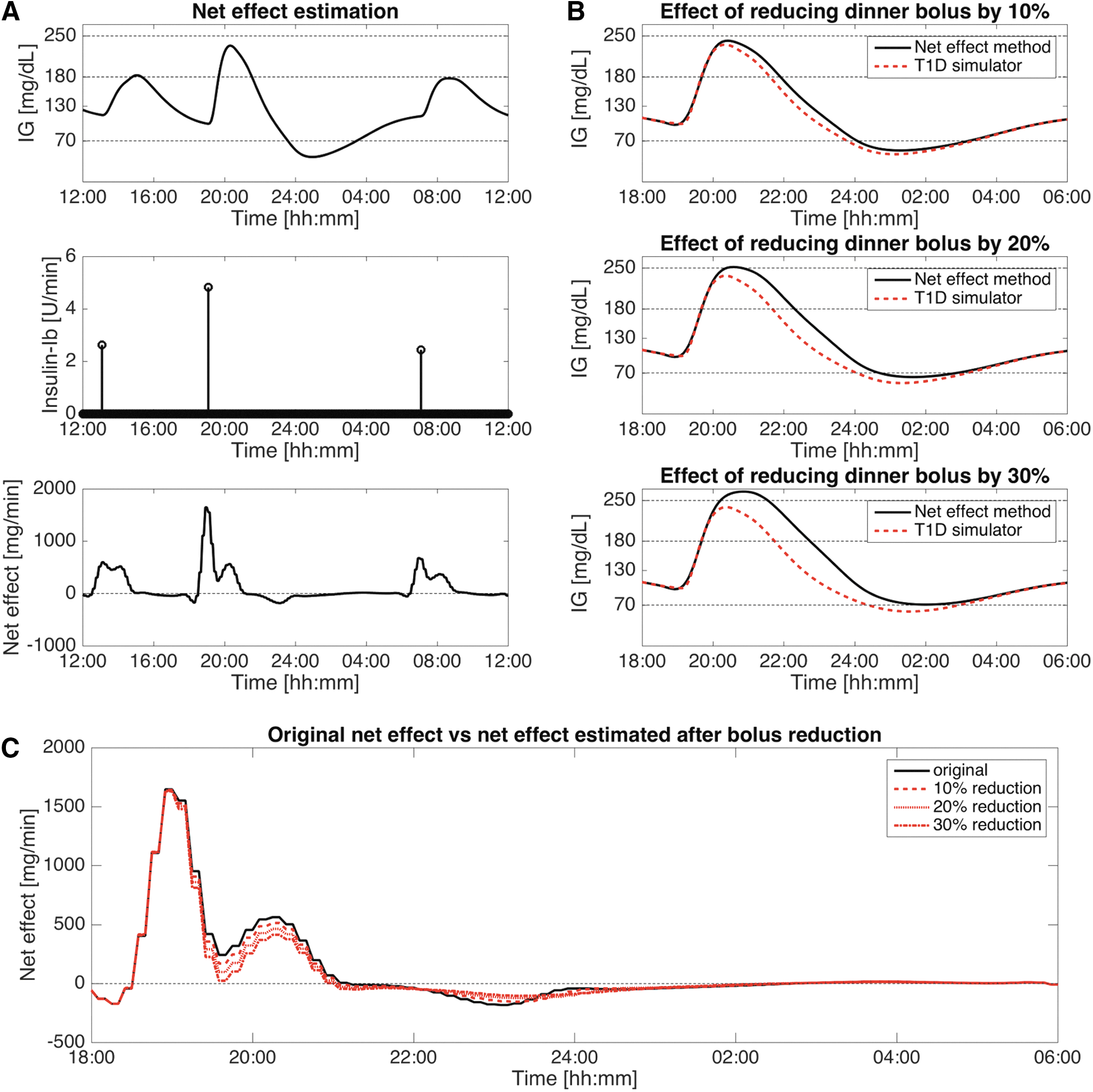
Case study 2 (modification of pre-existing boluses), virtual subject #2. (A) IG data (top), insulin data (middle), and estimated net effect (bottom) in a time frame of interest. (B) IG profile predicted by the net effect method (black solid line) and IG profile obtained by the UVA/Padova T1D simulator when dinner bolus is decreased by 10% (top), 20% (middle) and 30% (bottom). (C) Original net effect (black solid line) and net effect re-estimated after dinner bolus is decreased in the UVA/Padova simulator by 10% (red dashed line), 20% (red dotted line), and 30% (red dash-dot line). (Color graphics available at www.liebertonline.com/dia)

When the dinner bolus is reduced by 10% and 20%, the net effect method underestimates time in hypoglycemia of 0.5 and 0.9 h, respectively. When a 30% reduction is applied to the dinner bolus, while the net effect method predicts that such a reduction is sufficient to prevent the nocturnal hypoglycemia, in the UVA/Padova simulator a hypoglycemic event of duration 2.6 h is still present. The hypoglycemic event is prevented in the UVA/Padova T1D simulator only when the dinner bolus is reduced by at least 50% (results not shown). This means that the net effect method is significantly underestimating the reduction of the insulin bolus required to avoid the nocturnal hypoglycemia.

This case study confirms the criticality of one of the net effect method assumptions: the independence between the net effect and the insulin therapy. If this assumption were true, the net effect estimated from the original IG and insulin profile (Fig. 3C, black solid line) and the three net effects obtained after modifying the dinner bolus by −10%, −20%, and −30% in the UVA/Padova simulator (Fig. 3C, dashed, dotted, and dash-dot line, respectively) would be identical. However, as shown in Figure 3C, the assumption of independence between net effect and insulin therapy is not valid since the four net effect profiles are very different from each other.

Case study 3: Addition of new boluses

Virtual subject #3 presents hyperglycemia after breakfast (Fig. 4A, top panel). Let us use the net effect method to see the effect of adding a correction bolus, for example of 2 U, 2 h after breakfast (i.e., at 09:00) in response to a hyperglycemic alarm of the CGM sensor. After estimating the net effect trace (Fig. 4A, bottom panel) and adding the correction bolus to the original insulin therapy, the net effect method produces the IG profile reported by the black solid line in Figure 4B. When the same correction bolus is added to the insulin therapy used to generate the subject with the UVA/Padova simulator, the resulting IG profile is the one represented by red dashed line in Figure 4B.

FIG. 4.

Case study 3 (addition of new boluses), virtual subject #3. (A) IG data (top), insulin data (middle), and estimated net effect (bottom) in a time frame of interest. (B) IG profile predicted by the net effect method when a 2 U correction bolus is added at 09:00 (black solid line), and IG profile obtained when the same bolus is added in the UVA/Padova simulator (red dashed line). (C) Original net effect (black solid line) and net effect re-estimated after a 2 U correction bolus is added at 09:00 in the UVA/Padova simulator (red dashed line). (Color graphics available at www.liebertonline.com/dia)

In this study, the net effect method underestimates time in hyperglycemia of 1 h, since the correction bolus has a greater impact according to the net effect method than that it actually has in the UVA/Padova simulator. This discrepancy is likely due to an overestimation of the patient's insulin sensitivity in that particular period of the day and to the limitations of net effect model that is linearized about the basal state and does not properly take into account the inter- and intrasubject variability of physiology.

Again, if we compare the net effect profile estimated from original data (Fig. 4C, black solid line) and the one estimated from the IG profile obtained in the UVA/Padova simulator after adding the correction bolus (Fig. 4C, red dashed line), a significant difference between the two profiles can be noted between 09:00 and 11:00, which violates the assumption of independence between net effect and insulin therapy.

Case study 4: Addition of hypotreatments

In this study, we test the effect of adding a hypotreatment in response to a hypoglycemic alarm of the CGM sensor. Virtual subject #4 is a good candidate for such a purpose, since presenting a hypoglycemia around midnight (Fig. 5A, top panel). The net effect profile estimated from IG and insulin data is reported in Figure 5A, bottom panel. Since no information on how to add hypotreatments to the net effect is provided in Patek et al.,⁹ we decided to add an impulse to the net effect signal at the time in which IG crosses the hypoglycemic threshold (70 mg/dL) to simulate the intake of 15 g of carbohydrate (Fig. 5C, black solid line). The IG profile obtained by the modified net effect is reported in Figure 5B (black solid line), together with the IG profile simulated adding the 15 g hypotreatment in the UVA/Padova simulator (red dashed line).

FIG. 5.

Case study 4 (addition of hypotreatments), virtual subject #4. (A) IG data (top), insulin data (middle), and estimated net effect (bottom) in a time frame of interest. (B) IG profile predicted by the net effect method when a 15 g hypotreatment is added after IG crosses the hypoglycemic threshold (black solid line), and IG profile obtained in the UVA/Padova simulator when the same hypotreatment is introduced (red dashed line). (C) Original net effect with addition of a 15 g hypotreatment at 09:00 (black solid line), and net effect re-estimated after the same hypotreatment is added in the UVA/Padova simulator (red dashed line). (Color graphics available at www.liebertonline.com/dia)

The net effect method performs suboptimally also in this case by overestimating the time in hypoglycemia: when the hypotreatment is introduced in the UVA/Padova simulator, the duration of the hypoglycemic event is 21 min, while the time spent in hypoglycemia predicted by the net effect method is 67 min. This means, for instance, that the hypotreatment seems to be effective to limit the time spent in hypoglycemia by the patient, while the indication given by the net effect is the opposite. In line with the other three case studies, also here the net effect signal estimated from the IG profile obtained by the UVA/Padova simulator after the addition of the hypotreatment (Fig. 5C, red dashed line) presents significant differences compared to the original net effect (black solid line) both before and after the time of the hypotreatment.

Discussion

The net effect method proposed in Patek et al.⁹ is a promising tool for in silico testing of insulin therapies since it works retrospectively on real data collected by the patient and takes into account important components of BG variability, such as exercise, which are currently not included in T1D simulators. The net effect method has been recently used by Kovatchev et al.¹⁰ to assess the impact on glycemic control of various therapies based on the nonadjunctive use of CGM sensors. However, the possibility of reliably using the net effect method for testing insulin therapies outside modest changes of basal insulin delivery has not been assessed.

The aim here was to apply the net effect method to data simulated using the UVA/Padova simulator to test its ability to correctly predict the IG concentration that would result from real-life modifications of insulin therapies and, hence, determine the domain of validity of the method. Specifically, four case studies (resembling those used in Patek et al.⁹ and Kovatchev et al.¹⁰) were investigated: basal insulin modifications, changes of pre-existing boluses, addition of new boluses, and addition of new hypotreatments.

First, we noticed that the net effect signals (Figs. 2A, 3A, 4A, and 5A, bottom panels) are difficult to interpret, for example, they can take even negative values. Indeed, the net effect signal reflects physiological perturbations related to meals and other oscillations deriving from components of glucose variability not considered in the core linearized and discretized time-invariant model of the method.

The comparison with the reference provided by the simulator showed that the net effect method is able to reproduce quite accurately only the effect on IG concentration due to small adjustments of basal insulin (e.g., +10%, +20%, or −10%). However, when larger adjustments of basal insulin are performed (e.g., +50% or −20% and −50%) or boluses and hypotreatments are changed, the estimation of the IG profile by the net effect method is significantly different from that obtained by the UVA/Padova simulator. The discrepancies between the two IG profiles can be so important that inaccurate inferences on the modified insulin therapies may occur (see e.g., Case study 2).

The suboptimal behavior of the net effect method is caused by the many simplifications introduced in the patient model, such as the model linearization and absence of inter- and intrasubject variability of physiological parameters, and by the unrealistic assumption of independence between net effect and insulin therapy (see discrepancies observed in Figs. 2C, 2E, 3C, 4C, and 5C between the original net effect and the one re-estimated after introducing the therapy modifications in the UVA/Padova simulator).

In conclusion, the domain of validity of the net effect method seems to be limited to small variations of basal insulin, while in all the other scenarios, that is, larger adjustments of basal insulin (e.g., +50% and −50%) or changes of pre-existing boluses, addition of new boluses, and addition of new hypotreatments, the net effect is providing inaccurate results.

Footnotes

Author Disclosure Statement

No competing financial interests exist.

References

Cobelli

, Dalla Man

, Sparacino

, et al.: Diabetes: models, signals, and control. IEEE Rev Biomed Eng, 2009; 2:54–96.

Kovatchev

, Breton

, Dalla Man

, Cobelli

: In silico preclinical trials: a proof of concept in closed-loop control of type 1 diabetes. J Diabetes Sci Technol, 2009; 3:44–55.

Dalla Man

, Micheletto

, Breton

, et al.: The UVA/PADOVA type I diabetes simulator: new features. J Diabetes Sci Technol, 2014; 8:26–34.

Visentin

, Dalla Man

, Kovatchev

, et al.: The University of Virginia/Padova type 1 diabetes simulator matches the glucose traces of a clinical trial. Diabetes Technol Ther, 2014; 16:428–434.

Visentin

, Dalla Man

, Yogish

, et al.: Circadian variability of insulin sensitivity: physiological input for in silico artificial pancreas. Diabetes Technol Ther, 2015; 17:1–7.

Hovorka

, Canonico

, Chassin

, et al.: Nonlinear model predictive control of glucose concentration in subjects with type 1 diabetes. Physiol Meas, 2004; 25:905–920.

Wilinska

, Chassin

, Acerini

, et al.: Simulation environment to evaluate closed-loop insulin delivery systems in type 1 diabetes. J Diabetes Sci Technol, 2010; 4:132–144.

Kanderian

, Weinzimer

, Voskanyan

, Steil

: Identification of intraday metabolic profiles during closed-loop glucose control in individuals with type 1 diabetes. J Diabetes Sci Technol, 2009; 3:1047–1057.

Patek

, Lv

, Ortiz

, et al.: Empirical representation of blood glucose in a compartmental model. In: Kirchsteiger

, Jørgensen

, Renard

, del Re

, eds. Prediction Methods for Blood Glucose Concentration. Cham: Springer International Publishing, 2016.

10.

Kovatchev

, Patek

, Ortiz

, Breton

: Assessing sensor accuracy for non-adjunct use of continuous glucose monitoring. Diabetes Technol Ther, 2015; 17:1–10.

11.

Kovatchev

: Hypoglycemia reduction and accuracy of continuous glucose monitoring. Diabetes Technol Ther, 2015; 17:530–533.

12.

Castle

, Jacobs

: Nonadjunctive use of continuous glucose monitoring for diabetes treatment decisions. J Diabetes Sci Technol, 2016; 10:1169–1173

13.

Bailey

, Chang

, Christiansen

. Clinical accuracy of a continuous glucose monitoring system with an advanced algorithm. J Diabetes Sci Technol, 2015; 9:209–214.

14.

Peyser

, Nakamura

, Price

, et al.: Hypoglycemic accuracy and improved low glucose alerts of the latest dexcom G4 platinum continuous glucose monitoring system. Diabetes Technol Ther, 2015; 17:548–554.

15.

Cobelli

, Dalla Man

, Toffolo

, et al.: The oral minimal model method. Diabetes, 2014; 64:1203–1213.

16.

Visentin

, Dalla Man

, Kovatchev

, Cobelli

: Incorporation of intra-day variability into the UVA/Padova type 1 diabetes simulator. Diabetes Technol Ther, 2015; 17:A52–A53.

17.

Visentin

, Dalla Man

, Cobelli

: One-day Bayesian cloning of type 1 diabetes subjects: towards a single-day UVA/Padova type 1 diabetes simulator. IEEE Trans Biomed Eng, 2016; DOI: 10.1109/TBME.2016.2535241

18.

Vettoretti

, Facchinetti

, Sparacino

, Cobelli

: Accuracy of devices for self-monitoring of blood glucose: a stochastic error model. Conf Proc IEEE Eng Med Biol Soc, 2015; 2015:2359–2362.