Yet Another Glucose Variability Index: Time for a Paradigm Change?

Abstract

What is glucose variability (GV) and how can it be efficiently measured? The concept of GV is very intuitive. GV is how much the glucose signal varies in time and, thus, GV has two main components: the amplitude, which reflects the extent of blood glucose (BG) excursions, and timing, which reflects the frequency of BG variations. GV is becoming an important biomarker, which should be considered with other features, such as HbA1c, for a quantitative representation of diabetes mellitus.¹ In fact, HbA1c and GV from continuous glucose monitoring (CGM) data are expressions of the same underlying physiological process, evident on different timescale. HbA1c allows the assessment of long-term BG control,^2,3 but the evaluation of the risk of hypoglycemia requires other tools. Here, GV comes into play. In fact, both amplitude and frequency of BG fluctuations contribute to the risk of hypoglycemia, and the GV concept contains, in this definition, both these components.

However, how to efficiently measure GV is still an open question^4,5; tens of GV indices have been introduced. The start was on self-monitoring BG (SMBG) time series and indices such as standard deviation (SD), coefficient of variation (CV), and mean amplitude of glucose excursions (MAGE)⁶ were introduced. They all suffer the same strong limitation: they only consider the amplitude component of GV, without taking into account the frequency of glucose excursions. The focus on the amplitude component only is difficult to understand especially now in the era of CGM sensors, which allow observing glucose fluctuations that were impossible to be detected with SMBG, see for instance the point/counter-point by Service and Kovatchev^7,8 and the 2017 International Consensus on Use of Continuous Glucose Monitoring,⁹ which has recommended CV as the primary with SD as key secondary measure of GV. Fortunately, scientists have taken the new timing dimension made available by CGM into consideration and new metrics such as mean absolute glucose (MAG) change,¹⁰ mean of daily differences (MODD), and continuous overlapping net glycemic effect (CONGA)¹¹ have been developed.

The condensation into a single GV index of both amplitude and timing components of GV is quite challenging, in our opinion, almost impossible. First, from a pure mathematical point of view, since GV is a function of amplitude A and frequency of glucose excursions F, that is, GV = f(A,F), there could be infinite combinations of A and F that lead to the same GV value. Therefore, one single GV index does not appear to be the most efficient way to measure GV. Second, it is well known that the BG scale is highly asymmetric, and deviations toward hyperglycemia occupy a much wider range and are numerically “heavier” than deviations toward hypoglycemia.¹² As a result, SD, CV, MAGE, and MAG are inherently biased toward hyperglycemia and have a relatively weak association with hypoglycemia, which is often more clinically significant than hyperglycemia.

The glucose variability percent (GVP) metric presented by Peyser et al.¹³ is another metric added to the pool of GV indices, which tries to condensate into a single number the complexity of GV. GVP is not different from other available metrics, such as the distance travelled and MAG (a high correlation is expected although not shown). Also, it is unclear why the superiority of GVP versus CV, SD, and MAGE was claimed on the ability to discriminate among five diabetes subject cohorts: the primary purpose of GV is not classification—other measurements and methods are used—but assessing glucose control. In addition, the simulated examples are rather simplistic, do not reflect real-life glycemic traces, and one would have expected the use of more suitable in silico tools, for example, the UVA/Padova Type 1 Diabetes Simulator,¹⁴ which has been recently used by Dexcom, Inc. to create thousands of realistic multiple-day CGM traces to test safety and efficacy of the nonadjunctive use of the G5 Mobile sensor.^15
–17

The advent of CGM brings diabetes into a big data science context and, thus, advanced methods to quantify variability of the glucose dynamic stochastic processes are needed. It is our opinion that both amplitude and timing components of GV should be considered, but separately.

Measuring GV Amplitude

Given the asymmetry of the BG scale, the best metrics are those able to correct it, such as the low BG index, the high BG index, and the average daily risk range, which are all easy to compute.¹²

In addition, a useful tool to visualize the amplitude of glucose excursions is the Variability Grid Analysis (VGA), which is a minimum/maximum plot of the BG readings for a subject taken over a certain observation period.¹⁸ The minimum BG (the lower 2.5th percentile) is plotted on the x-axis, which ranges from 110 to <50 mg/dL. The maximum BG (the upper 2.5th percentile) is plotted on the y-axis. The plot is split into nine zones: A-zone (green) indicates optimal control; the B-zones (dark green) are good, but suboptimal, control; C-zone (yellow) indicates overcorrection of hypoglycemia or hyperglycemia; and D-zone (orange) indicates even higher degree of GV, while E-zone (red) a very poor glucose control. An example of the application of VGA on two representative subjects is shown on the top panel of Figure 1.

FIG. 1.

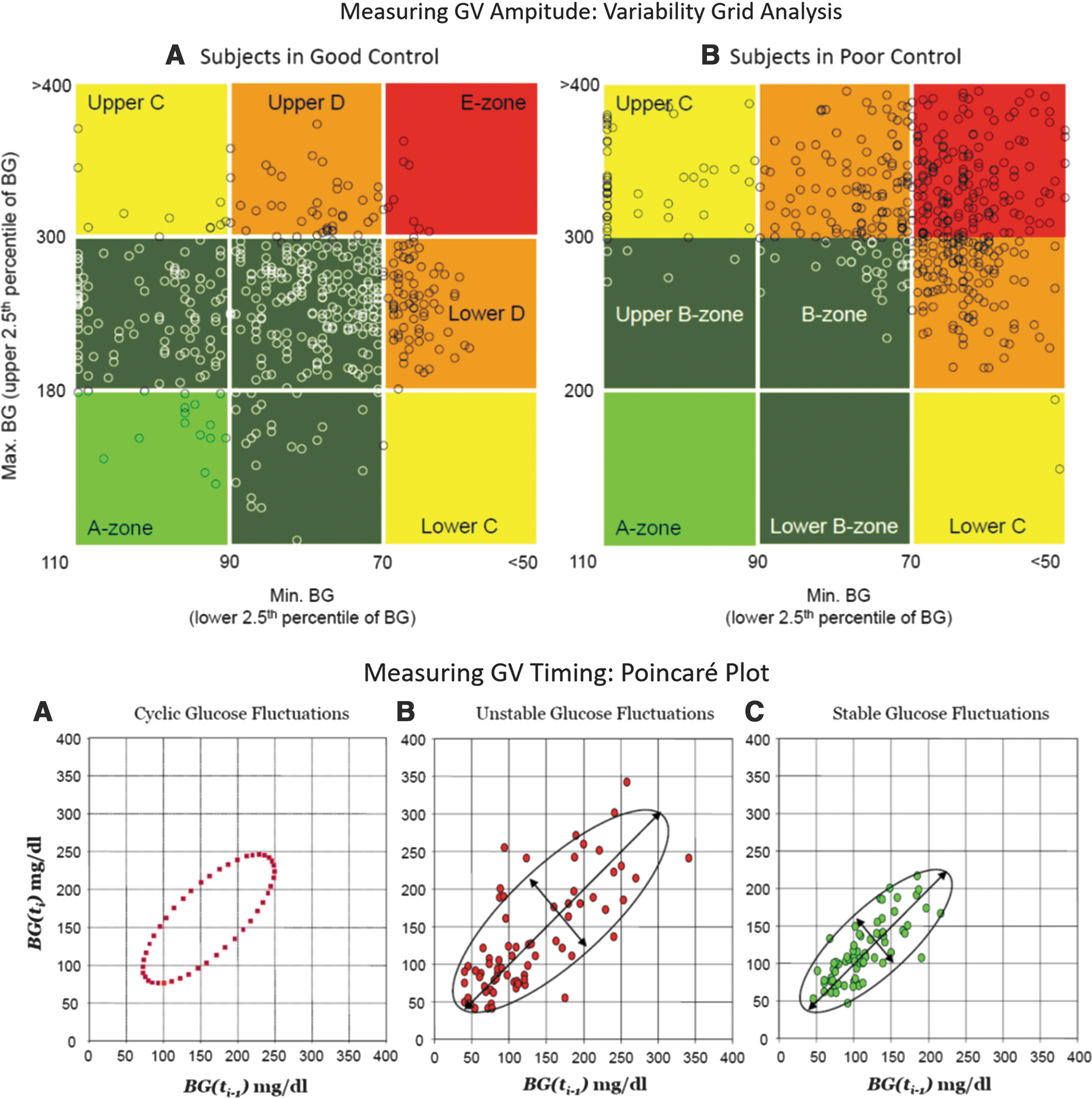
Top: Variability Grid Analysis. Each data point has coordinates (minimum and maximum) BG for a subject during the observation period. Subjects in (A) are in good control with most of the data points in A- and B-zones; Subjects in (B) are in poor control with most of the data points in C-, D-, and E-zones. Bottom: Poincaré plot of BG fluctuations depicting system dynamics. (A) Presents the plot of perfectly cyclic glucose fluctuations—an unrealistic, but illustrative scenario; (B) presents unstable BG fluctuations of a person in poor control; and (C) presents stable BG fluctuations of a person in good control. Both figures are taken from Ref.5. BG, blood glucose.

Measuring GV Timing

The calculation of the simple, readily understandable % time in range (70–180 mg/dL),% time in hypoglycemia (below 70 mg/dL), and % time in hyperglycemia (above 180 mg/dL) is the most straightforward way to assess the timing component of GV. On the other hand, MODD, which allows focusing on interday glycemic variations, and CONGA, which aims at calculating the SD of the differences between BG readings collected some hours apart, are useful metrics to measure the temporal (periodical) characteristics of BG dynamics.¹¹

The Poincaré plot of glucose dynamics is a useful tool to visualize the timing component of GV and the risk for hypoglycemia and hyperglycemia over time,¹⁸ in which each point has coordinates the BG value measured at time t+1 on the x-axis and the BG measured at time t on the y-axis. Examples of Poincaré plots of BG reading are shown on the bottom panel of Figure 1: an elliptic plot refers to an oscillating system (Fig. 1A) and a concentrated plot reflects a stable patient with good control in time (Fig. 1B), while a scatter plot refers to a patient with poor glycemic control (Fig. 1C).

To conclude, we would like to offer some general comments in these times of big data science and precision medicine. GV quantitative assessment is not straightforward because glucose fluctuations carry two components: amplitude and timing. The standard assessment of GV originated by SMBG is measuring amplitude, but the timing of BG fluctuations is crucial and with availability of big data provided by CGM, the assessment of GV timing is not only possible but also mandatory. Fortunately, the fields of time series and dynamical systems analysis are highly developed; the computational methods are standardized and available in a number of software products, and there is no excuse for not using them to assess the timing component of GV. We should emphasize that diabetes is among the diseases that have most benefitted from advanced modeling and computing methods.¹⁹ For instance, the minimal model of glucose–insulin dynamics has been used for over 30 years to assess insulin sensitivity and beta cell function.²⁰ In this commentary, we call for a paradigm change and argue that techniques known in mathematics for decades can be very beneficial to assess the amplitude and timing components of GV. GV can help to better evaluate new medications, which specifically target restoration of normal BG fluctuations on timescales that are well beyond the resolution of HbA1c. Similarly, artificial pancreas algorithms rely on metrics of GV to set their glycemic targets and optimize insulin delivery in real time; thus, judging the efficacy of artificial pancreas systems solely from the point of view of improvements in levels of HbA1c might miss many benefits that closed-loop control systems can provide. Thus, we hope this commentary will help standardizing, by scientific consensus, of the advanced methods for assessment of the components of GV.

Footnotes

Author Disclosure Statement

C.C. holds patent applications in diabetes technology, and received research support and material from Dexcom. A.F. holds patent applications in diabetes technology, and received research support and material from Dexcom.

References

Cryer

: Glycemic goals in diabetes: trade-off between glycemic control and iatrogenic hypoglycemia. Diabetes, 2014; 63:2188–2195.

Svendsen

, Lauritzen

, Søegaard

, Nerup

: Glycosylated haemoglobin and steady-state mean blood glucose concentration in Type 1 (insulin-dependent) diabetes. Diabetologia, 1982; 23:403–405.

Santiago

: Lessons from the diabetes control and complications trial. Diabetes, 1993; 42:1549–1554.

Kovatchev

: Metrics for glycaemic control—from HbA1c to continuous glucose monitoring. Nat Rev Endocrinol, 2017; 13:425–436.

Kovatchev

, Cobelli

: Glucose variability: timing, risk analysis, and relationship to hypoglycemia in diabetes. Diabetes Care, 2016; 39:502–510.

Service

, Molnar

, Rosevear

, et al.: Mean amplitude of glycemic excursions, a measure of diabetic instability. Diabetes, 1970; 19:644–655.

Service

: Comment on Kovatchev and Cobelli. Glucose variability: timing, risk analysis, and relationship to hypoglycemia in diabetes. Diabetes Care, 2016; 39:502–510.

Kovatchev

, Cobelli

: Response to Comment on Kovatchev and Cobelli. Glucose variability: timing, risk analysis, and relationship to hypoglycemia in diabetes. Diabetes Care, 2016; 39:502–510.

Danne

, Nimri

, Battelino

, et al.: International Consensus on Use of Continuous Glucose Monitoring. Diabetes Care, 2017; 40:1631–1640.

10.

Hermanides

, Vriesendorp

, Bosman

, et al.: Glucose variability is associated with intensive care unit mortality. Crit Care Med, 2010; 38:838–842.

11.

McDonnell

, Donath

, Vidmar

, et al.: A novel approach to continuous glucose analysis utilizing glycemic variation. Diabetes Technol Ther, 2005; 7:253–263.

12.

Kovatchev

, Cox

, Gonder-Frederick

, Clarke

: Symmetrization of the blood glucose measurement scale and its applications. Diabetes Care, 1997; 20:1655–1658.

13.

Peyser

, Balo

, Buckingham

, et al.: Glycemic variability percentage: a novel method for assessing glycemic variability from continuous glucose monitor data. Diabetes Technol Ther, 2018; 20:6–16.

14.

Dalla Man

, Micheletto

, Lv

, et al.: The UVA/PADOVA type 1 diabetes simulator: new features. J Diabetes Sci Technol, 2014; 8:26–34.

15.

Edelman

: Regulation catches up to reality. J Diabetes Sci Technol, 2017; 11:160–164.

16.

FDA Advisory Panel Votes to Recommend Non-Adjunctive Use of Dexcom G5 Mobile CGM. Diabetes Technol Ther, 2016; 18:512–516.

17.

Vettoretti

, Facchinetti

, Sparacino

, Cobelli

: Type 1 diabetes patient decision simulator for in silico testing safety and effectiveness of insulin treatments. IEEE Trans Biomed Eng, 2017. doi: 10.1109/TBME.2017.2746340.

18.

Clarke

, Kovatchev

: Statistical tools to analyze continuous glucose monitor data. Diabetes Technol Ther, 2009; 11 Suppl 1:S45–S54.

19.

Cobelli

, Man

, Pedersen

, et al.: Advancing our understanding of the glucose system via modeling: a perspective. IEEE Trans Biomed Eng, 2014; 61:1577–1592.

20.

Cobelli

, Dalla Man

, Toffolo

, et al.: The oral minimal model method. Diabetes, 2014; 63:1203–1213.