Green Space and Inequities in Healthy Ageing: Are Grasses Greener on the Socioeconomically Advantaged Side?

Abstract

Despite emerging evidence that green space is beneficial for all, there is little evidence comparing the association of green space with healthy ageing outcomes for people with socioeconomic advantages and those without such privileges. This article investigates the association between green space availability and healthy ageing outcomes for disadvantaged socioeconomic groups relative to privileged counterparts. Green space was classified as grass, low-lying vegetation, and tree canopy. Healthy ageing indices were calculated for 34,085 participants in the Sax Institute's 45 and Up Study (baseline 2006–2009), New South Wales, Australia. Partitioning was by socioeconomic and demographic characteristics and the association was assessed using regression analysis. Increasing grass cover was associated with declining health after age 45 years. Increasing low-lying vegetation (>10%) was associated with increased functional capacity but not resilience or healthy ageing. Green space association with the healthy ageing score was higher for widows (β 0.013, 95% CI 0.00–0.03) compared with individuals with a partner (β 0.003, 95% CI 0.00–0.01). Also, the association was higher for participants earning <$20k/annum (β 0.015, 95% CI 0.01–0.02) versus those earning >$70k (β 0.007, 95% CI 0.00–0.01). This beneficial association was higher for participants with no academic qualifications (β 0.021, 95% CI 0.01–0.04) and for participants who are disabled (β 0.028, 95% CI 0.00–0.06) in their respective groups. Green space contributes more to the healthy ageing of disadvantaged groups than affluent groups. Targeted investment in green space provision, especially tree canopy >30%, can be readily leveraged to provide beneficial health outcomes and reduce the effect of socioeconomic disparity for disadvantaged communities.

Introduction

Green space refers to an area of land with trees, grass, or other vegetation allocated for recreational or aesthetic purposes in or adjoining an urban area (Taylor & Hochuli, 2017). There is increasing evidence about the beneficial influence of green space, an important part of the natural environment in the neighborhood, on people's health and well-being (Clarke & Nieuwenhuijsen, 2009; de Keijzer, Bauwelinck & Dadvand, 2020; Markevych et al., 2017).

This is because neighborhood green space provides a beneficial public health amenity such as a place for socializing, exercise, play, recreation, and relaxation for all (Frumkin, 2001; Hartig, Mitchell, De Vries, & Frumkin, 2014; Pearce, Shortt, Rind, & Mitchell, 2016). In addition, for the elderly, increasing coverage of green space in the neighborhood was found to be associated with increased physical functioning (de Keijzer et al., 2019; Gong, Gallacher, Palmer, & Fone, 2014), better mental health (Astell-Burt, Mitchell, & Hartig, 2014), and cognitive function (Brown et al., 2018; Cherrie et al., 2018).

Healthy ageing is the process of developing and maintaining the functional ability that enables well-being in older age (Beard et al., 2016). In this research, it is measured by the Healthy Ageing Score (HAS), an aggregate of the domains that are relevant to ageing well (John, Astell-Burt, Yu, Brennan-Horley, & Feng, 2021). The HAS comprises physical function, cognitive function, balance and falls, mental health, sleep, quality of life/optimism, and social connection. It considers other factors in a person's environment that may impact their day-to-day life (National Disability Insurance Scheme, 2020).

The HAS can be subdivided into two domains: functional capacity and resilience. Functional capacity has four items: physical function, cognitive function, balance, and falls. Resilience also has four items: mental health, sleep, quality of life/optimism, and social connection. Current healthy ageing research focuses on health outcomes and perceived well-being (de Keijzer, Bauwelinck, & Dadvand, 2020) and has not fully utilized an aggregate measure of healthy ageing comparable for individuals and groups. The HAS in this study provides a holistic impression of neighborhood green space on health disparity at old age for different socioeconomic and demographic groups.

A disadvantaged group is a group of people who are limited or deprived of the privileges and rights of participating or benefitting from society due to their physical, mental, social, economic, educational, racial, cultural, religious, or environmental circumstances (Unegbu, 2012). Green space is known to be beneficial for the socioeconomically disadvantaged, who may use more ecosystem services provided by the green space than their counterparts with better access to other resources (Lin, Fuller, Bush, Gaston, & Shanahan, 2014; Mitchell, Richardson, Shortt, & Pearce, 2015; Thompson et al., 2012; Zandieh, Martinez, & Flacke, 2019).

One recent systematic review found that the associations between green space and several physical health outcomes are stronger and/or more consistent for disadvantaged people than for more advantaged groups, especially in Europe (Rigolon, Browning, McAnirlin, & Yoon, 2021). The reviewers synthesized evidence that, compared with privileged groups, disadvantaged groups had less wealth, less health care, and reduced access to urban green space, and are disproportionately exposed to hazardous residential and work environments with increased air pollution, noise, and heat.

These disparities in hazardous environmental exposure result in disparities in health outcomes that can be quite systemic (Braveman, Arkin, Orleans, Proctor, & Plough, 2017; National Academies of Sciences Engineering and Medicine 2017; Woolf & Braveman, 2011). Whether these disparities persist into old age is yet to be established. Another study reported that a deprived urban population of middle-aged adults who were out of a job experienced less stress when exposed to higher levels of surrounding green space (Roe et al., 2013). Another study also found the association between reduced premature circulatory death and increased green space access in socioeconomically deprived populations (Lachowycz & Jones, 2014).

From the foregoing, investigators have tried to unravel and understand the disparities in terms of specific health outcomes between the wealthy and the disadvantaged grounded on green space exposure around. Aside from the ethical concerns, identifying any disparities in overall healthy ageing due to inequities in green space exposure is important in designing environmental interventions to mitigate environmental hazards and providing protective effects to foster health equity (Jennings, Baptiste, Jelks, & Skeete, 2017). Therefore, we are also interested in uncovering the triangular relationships among green space types, holistic healthy ageing, and socioeconomic status. Within the socioeconomically deprived groups, it is also important to unlock any moderating effect on the association of green space and healthy ageing by individual's level of education, income, or employment status.

Green space is not uniform and can vary considerably based on its foliage, coverage, and density features. Green space can be classified into three types: grass, low-lying vegetation, or tree canopy. Astell-Burt and Feng (2019) classified the coverage of each vegetation type and found that different types of green space have different associations with health and well-being. The effect of different types of green space on health outcomes has been shown to be quite different. Tree canopy has been shown to lower dementia risk (Astell-Burt, Navakatikyan, & Feng, 2020), lower the odds of depression (Nishigaki, Hanazato, Koga, & Kondo, 2020), support physical activity (Feng, Toms, & Astell-Burt, 2021), and mitigate heat distress (Venter, Krog, & Barton, 2020) when compared with lower-lying vegetation and grass. No work has shown if this effect of tree canopy extends to a composite healthy ageing measure.

Aim of this study

Green space near people's homes has the potential to mitigate health inequalities in cardiovascular health, chronic medical conditions, and mental health in older people due to socioeconomic deprived groups compared with the well-off (Brown et al., 2016, 2018; Kling, 2018). It has also suggested that improving local resources can compensate for the reduced opportunity of long-distance travel for the socioeconomically deprived group, which may further reduce inequality (Maas et al., 2009; Mitchell & Popham, 2008). Therefore, this study aims to evaluate the health effect of different types of green spaces on socioeconomically disadvantaged groups. The following hypotheses were tested:

Hypothesis 1: There is a stronger association between neighborhood green space and healthy ageing for disadvantaged groups than privileged groups.

Hypothesis 2: Different types of neighborhood green spaces have different associations with healthy ageing.

Materials and Methods

Data

Ethics approval for this project was acquired from the University of Wollongong Human Research Ethics Committee. The cohort data were extracted in January 2019 from the Sax Institute's 45 and Up Study, Australia's largest ongoing study of health and ageing for 15 years. The data set we used was extracted from 267,153 participants living in the cities of Sydney, Wollongong, and Newcastle, Australia between 2006 and 2009, with data for all health outcome measures that comprise the HAS. This study included 34,085 participants who had data for calculating HAS and green space types. The Department of Human Services (formerly Medicare Australia) enrolment database was originally used to randomly sample and then recruit participants at baseline using a postal survey that provided near-complete coverage of the population of Australia (45 and Up Study Collaborators et al., 2008).

Outcome variables

Healthy ageing was measured by the HAS. The score ranges from 0 to 16, with higher scores indicating preferable ageing. Any participant who exceeded the recommended threshold for each domain item was given a high score of 2, a moderate score of 1 if they meet the recommendation, and a low score of 0 if they did not meet the recommended guideline. The HAS and its latent structures of functional capacity and resilience were the outcome variables.

Green space exposure variables

Green space can be measured using satellite imagery or records of land allocation. Most epidemiological research uses remote sensing satellite imagery to compute the normalized difference vegetation index or other indices (Nguyen Astell-Burt, Rahimi-Ardabili, & Feng, 2021). This index is helpful in identifying the location of green space, but it does not describe the density structure in areas of high vegetation coverage due to saturation (Prabhakara, Hively, & McCarty, 2015). However, Geovision© raster data (supplied by Pitney Bowes Ltd for 2016) classifies green space based on density and foliage into grass cover, low-lying vegetation, and tree canopy as a percentage of land cover within 1.6 km (1 mile) of the participant's residence.

This approach was chosen so that the effect of different green space types on healthy ageing and its different domains can be obtained. Green space data were obtained from the centroid of the “meshblock” of residence of each participant. These data described publically accessible discrete green spaces (e.g., parks) but did not include street trees, agricultural land, or private gardens. The percentage of green space coverage was calculated within buffers of 1600 m radius about the respondent's residence. This is a standard distance used to approximate a zone of roughly 20-min walk (Ekkel & de Vries, 2017).

Green space variables were tested as continuous variables and in categories (total green space 0–4%, 5–9%, 10–19%, 20–29%, ≥30%; tree canopy 0–9%, 10–19%, 20–29%, ≥30%; low-lying vegetation 0–4%, 5–9%, ≥10%; grass cover space 0–4%, 5–9%, 10–19%, 20–29%, ≥30%). The selection of these categories was a priori and based on existing green space standards in Perth (Western Australia), where ∼10% of subdivisible land is allocated to some form of green open space. Indicators of grass and low-lying vegetation are underestimated because they refer only to those provisions that were not beneath the tree canopy (Astell-Burt & Feng, 2019).

Socioeconomic variables and confounders

Age, gender, couple status, income, highest education, and employment were controlled for as potential level 1 confounders in the models in line with previous research (Astell-Burt, Feng, & Kolt, 2014; Bartram, 2021). Neighborhood disadvantage was controlled for using Deciles of Relative Socioeconomic Disadvantage of the neighborhoods where participants lived as a level 2 covariate to ensure that the observed associations with the HAS and its dimensions were attributable to types of green space. The highest educational attainment was selected as the key interaction variable for determining and comparing socioeconomic advantage or disadvantage as education is strongly associated with better health and wealth outcomes (Raghupathi & Raghupathi, 2020; Strulik, 2018; Zajacova & Lawrence, 2018).

Some studies have used income as a determinant of advantage/disadvantage. Still, we chose to use education in this article because several prior Australian studies have shown that increasing educational attainment is associated with higher median total income and income from wages and salaries (Leigh, 2008; Leigh & Ryan, 2005). For example, the Australia Department of Education reported that Australians with a doctorate are up to six times more likely to be in the top 10% of all incomes in Australia compared with other levels of educational attainment. They are also significantly less likely to receive the aged pension upon retirement (Department of Education, 2019).

Significant interactions between education and green space types were reported.

Statistical analysis

Summary statistics and multilevel models with interactions were used to assess and compare the distribution and influence of available green space on healthy ageing in the various population subgroups. We partitioned the sample according to gender and reported the association of total green space with functional capacity, resilience, and HAS while controlling for age, couple status, employment status, household income, and education. Next we partitioned the sample by age and reported the association of total green space with functional capacity, resilience, and HAS while controlling for gender, couple status, employment status, household income, and education. We continued in this manner till we partitioned the sample by education and reported the association of total green space with functional capacity, resilience, and HAS while controlling for age, gender, couple status, employment status, and household income. The associations are shown in Table 2 and Figure 2.

To investigate this clustering association, a linear two-level multilevel model was fitted with the SA2 as the level 2 ( $n_{S A 3}$ = 90) geographical clustering variable. The study participant was set to level 1 in the model (n = 34,085), with the HAS and its dimensions as the response variable. SA2s hold an average population of 10,000 and was developed by the Australian Bureau of Statistics to approximate local communities (Australian Bureau of Statistics, 2016). Next multilevel models were applied to estimate the association between green space types and healthy ageing for the whole sample. Two-way interaction terms between green space types and educational attainment were included to the model and likelihood ratio tests were conducted to assess model performance. All analysis was conducted in Stata 16 (StataCorp, 2007).

Results

Table 1 shows the partitions of the study sample, the mean functional capacity, mean resilience, mean HAS, and mean green space exposure of the subgroups. The ANOVA test showed that the mean functional capacity, resilience, HAS, and green space exposure for each subgroup were significantly different except for the mean green space exposure for areas with low lying vegetation, gender, and couple status. This means that there was no distinguishable difference in the green space exposure between men and women as well as between single, married/with partner, widowed, divorced, or separated individuals.

Table 1.

Distribution of Functional Capacity, Resilience, and Healthy Ageing Score by Green Space Types in the Study

CHARACTERISTIC	BASELINE TOTAL	MEAN FUNCTIONAL CAPACITY (SD)	MEAN RESILIENCE (SD)	MEAN HAS (SD)	DISCRETE GREEN SPACE
Total green space %	34,085	6.36 (0.009)	7.57 (0.003)	13.89 (0.008)	12.42 (0.045)
		^a	^a	^a
0 − 4	—	—	—	—	—
5–9	4	7.00 (0.577)	8.00 (0.000)	15.00 (0.577)	—
10–19	457	6.19 (0.088)	7.43 (0.043)	13.63 (0.122)	—
20–29	7799	6.27 (0.020)	7.49 (0.010)	13.76 (0.026)	—
≥30	25,825	6.392 (0.011)	7.59 (0.005)	13.98 (0.013)	—
% Grass		^a	^a	^a
0 − 4	1646	6.61 (0.039)	7.62 (0.018)	14.23 (0.047)	—
5–9	16,217	6.47 (0.013)	7.59 (0.006)	14.04 (0.016)	—
10–19	9447	6.33 (0.018)	7.55 (0.008)	13.88 (0.023)	—
20–29	5331	6.12 (0.026)	7.49 (0.012)	13.61 (0.032)	—
≥30	1444	6.14 (0.049)	7.52 (0.022)	13.66 (0.061)	—
% Low-lying vegetation			^a	^a
0–4	15,936	6.37 (0.014)	7.55 (0.006)	13.93 (0.017)	—
5–9	16,949	6.35 (0.013)	7.57 (0.006)	13.92 (0.016)	—
≥10	1200	6.38 (0.049)	7.60 (0.022)	13.98 (0.059)	—
% Tree canopy		^a	^a	^a
0–9	2843	5.98 (0.037)	7.40 (0.019)	13.38 (0.005)	—
10–19	12,995	6.22 (0.016)	7.50 (0.008)	13.73 (0.020)	—
20–29	8953	6.43 (0.018)	7.60 (0.008)	14.03 (0.022)	—
≥30	9294	6.60 (0.016)	7.65 (0.007)	14.25 (0.019)	—
Gender		^a	^a	^a
Male	36,661	6.45 (0.013)	7.55 (0.006)	14.00 (0.016)	12.51 (0.067)
Female	44,164	6.28 (0.013)	7.57 (0.006)	13.86 (0.017)	12.34 (0.061)
Age group (years)		^a	^a	^a	^a
45–54	9968	6.72 (0.015)	7.51 (0.008)	14.23 (0.019)	12.43 (0.081)
55–64	11,388	6.57 (0.015)	7.60 (0.007)	14.17 (0.019)	12.65 (0.079)
65–74	7260	6.29 (0.020)	7.65 (0.009)	13.93 (0.024)	12.62 (0.100)
75+	5469	5.35 (0.028)	7.48 (0.012)	12.83 (0.035)	11.67 (0.109)
Couple status		^a	^a	^a
Single	1961	6.22 (0.041)	7.44 (0.021)	13.67 (0.053)	11.38 (0.161)
Married/with partner	25,921	6.49 (0.010)	7.59 (0.005)	14.08 (0.012)	12.61 (0.053)
Widowed	2823	5.47 (0.040)	7.48 (0.020)	12.96 (0.050)	11.86 (0.149)
Divorced	2476	6.20 (0.037)	7.49 (0.018)	13.68 (0.047)	12.18 (0.149)
Separated	752	6.15 (0.066)	7.39 (0.037)	13.54 (0.087)	11.80 (0.267)
Economic status		^a	^a	^a	^a
Employed	11,193	6.87 (0.012)	7.56 (0.007)	14.43 (0.015)	12.50 (0.077)
Unemployed	417	5.71 (0.100)	7.18 (0.058)	12.89 (0.138)	11.87 (0.341)
Retired	10,841	5.90 (0.018)	7.58 (0.008)	13.48 (0.022)	12.45 (0.082)
Disabled	489	3.16 (0.100)	6.26 (0.074)	9.41 (0.148)	12.33 (0.079)
Annual household income		^a	^a	^a	^a
<$20k	4537	5.28 (0.032)	7.30 (0.016)	12.58 (0.042)	12.20 (0.117)
$20–$40k	4904	6.08 (0.026)	7.56 (0.012)	13.64 (0.031)	12.35 (0.115)
$40–$70k	18,206	6.76 (0.010)	7.63 (0.005)	14.39 (0.013)	12.54 (0.063)
>$70k	5778	6.25 (0.024)	7.56 (0.011)	13.81 (0.029)	12.30 (0.109)
Education		^a	^a	^a	^a
None	2222	5.25 (0.047)	7.20 (0.025)	12.46 (0.063)	12.18 (0.164)
School or intermediate certificate	5654	6.11 (0.024)	7.57 (0.011)	13.68 (0.030)	12.71 (0.110)
Higher school or leaving certificate	3187	6.26 (0.031)	7.56 (0.014)	13.82 (0.038)	12.07 (0.139)
Trade or apprenticeship	2893	6.09 (0.033)	7.54 (0.015)	13.64 (0.040)	12.54 (0.153)
Certificate or diploma	7834	6.42 (0.019)	7.60 (0.008)	14.02 (0.023)	12.50 (0.095)
University degree or higher	11,974	6.75 (0.013)	7.61 (0.006)	14.36 (0.016)	12.32 (0.078)

Significant difference in the means of the categories by ANOVA, α = 5%, n = 34,085.

HAS, healthy ageing score.

Areas that had 30% or more of greenery comprising tree canopy reported the highest surrounding green space, mean functional capacity, mean resilience, and ultimately highest mean HAS. In the partitions with significant differences in mean functional capacity, the participants who are employed 6.87 (0.012), earning between $40k and $70k 6.76 (0.010), bachelors and postgraduate degree holders 6.75 (0.013), aged 45–54 years 6.72 (0.015), married or living with a partner 6.49 (0.01), and men 6.45 (0.013) reported the highest functional capacity in that order and disabled participants had the lowest functional capacity.

When examining resilience, participants aged 65–74 years 7.65 (0.009), with annual household incomes of $40k–$70k 7.63 (0.005), completed a bachelor or postgraduate degree 7.61 (0.006), married or living with a partner 7.59 (0.005), retired 7.58 (0.008), and female 7.57 (0.006) reported the highest mean scores for resilience in that order. Disabled participants had the least mean resilience of 6.26 (0.074).

Participants who were employed 14.43 (0.015), with an annual household income of $40k–$70k (14.39), completed a bachelor or postgraduate degree 14.36 (0.016), aged between 45 and 54 years 14.39 (0.013), married or living with a partner 14.08 (0.012), and men 14.00 (0.016) reported the highest mean HAS in that order, whereas disabled participants reported the lowest average HAS (9.41). The results in Table 1 revealed that the following categories, within their groups, reported the highest percentage of total green space within a 1600 m radius of their residences: males 12.51 (0.067), aged between 55 and 64 years 12.65 (0.079), married/with a partner 12.61 (0.058), employed 12.50 (0.077), earning between 40k and 70k 12.54 (0.063), and being a tradesperson or apprentice 12.54 (0.153).

Conversely, Table 2 shows the groups with significant associations between total green space and functional capacity and healthy ageing. The groups were 65–74 year olds 0.006 (0.00, 0.01), widows 0.01 (0.00, 0.02), disabled 0.028 (0.00, 0.06), and individuals with no academic qualifications 0.014 (0.00, 0.03). Also, the groups that reported the strongest significant association between total green space and resilience were females 0.002 (0.001, 0.003), married/with partner 0.001 (0.00), employed 0.002 (0.00, 0.01), and participants with no academic qualifications 0.007 (0.00, 0.01).

Table 2.

Adjusted Association of Total % Green Space with Functional Capacity, Resilience and Healthy Ageing Score from Separate Models Partitioned Samples for Age, Gender, Couple Status, Economic Status, Annual Household Income, and Education

CHARACTERISTICS	OUTCOME
CHARACTERISTICS	FUNCTIONAL CAPACITY ASSOCIATION OF % GREEN SPACE (95% CI)	RESILIENCE ASSOCIATION OF % GREEN SPACE (95% CI)	HAS ASSOCIATION % OF GREEN SPACE (95% CI)
Gender
Male	0.002 (−0.00 to 0.01)	0.001 (0.00)	0.003 (0.00 to 0.01)
Female	0.002 (−0.00 to 0.01)	0.002 (0.00)^a	0.004 (0.00 to 0.01)^a
Age group (years)
45 to 54	0.000 (0.00)	0.001 (0.00)	0.002 (−0.00 to 0.01)
55 to 64	0.001 (0.00)	0.001 (0.00)	0.002 (−0.00 to 0.01)
65 to 74	0.006 (0.00 to 0.01)^a	0.002 (0.00)	0.008 (0.00 to 0.01)^a
75+	0.003 (−0.00 to 0.01)	0.001 (0.00)	0.004 (−0.00 to 0.01)
Couple status
Single	0.004 (−0.00 to 0.01)	0.004 (−0.00 to 0.01)	0.008 (−0.01 to 0.02)
Married/with partner	0.002 (0.00)	0.001 (0.00)^a	0.003 (0.00 to 0.01)^a
Widowed	0.01 (0.00 to 0.02)^a	0.003 (−0.00 to 0.01)	0.013 (0.00 to 0.03)^a
Divorced	−0.0001 (−0.01 to 0.01)	−0.001 (−0.01 to 0.00)	−0.0006 (−0.01 to 0.01)
Separated	−0.003 (−0.02 to 0.01)	0.001 (−0.00 to 0.01)	−0.002 (−0.02 to 0.02)
Employment status
Employed	0.001 (0.00)	0.002 (0.00 to 0.01)^a	0.004 (0.00 to 0.01)
Unemployed	0.015 (−0.01 to 0.04)	−0.002 (−0.02 to 0.01)	0.013 (−0.02 to 0.05)
Retired	0.004 (0.00 to 0.01)^a	0.001 (0.00)	0.005 (0.00 to 0.01)^a
Disabled	0.028 (0.00 to 0.06)^a	0.005 (−0.02 to 0.03)	0.033 (−0.01 to 0.08)
Annual household income
<$20k	0.011 (0.00 to 0.02)^a	0.004 (0.00 to 0.01)	0.015 (0.01 to 0.02)^a
$20 to $40k	0.003 (0.00 to 0.01)	0.001 (0.00 to 0.00)	0.003 (0.00 to 0.01)
$40 to $70k	0.000 (0.00 to 0.00)	0.001 (0.00 to 0.00)	0.001 (0.00)
>$70k	0.005 (0.00 to 0.01)^a	0.002 (0.00 to 0.00)	0.007 (0.00 to 0.01)^a
Education
None	0.014 (0.00 to 0.03)^a	0.007 (0.00 to 0.01)^a	0.021 (0.01 to 0.04)^a
School or intermediate certificate	0.003 (−0.00 to 0.01)	0.003 (0.00 to 0.01)^a	0.006 (−0.00 to 0.01)
Higher school or leaving certificate	0.004 (−0.00 to 0.01)	0.001 (0.00)	0.004 (−0.00 to 0.01)
Trade or apprenticeship	−0.0002 (−0.01 to 0.01)	0.002 (−0.00 to 0.01)	0.002 (−0.00 to 0.01)
Certificate or diploma	−0.0003 (0.00)	−0.0004 (0.00)	−0.001 (−0.01 to 0.00)
University degree or higher	0.003 (−0.00 to 0.01)	0.001 (0.00)	0.003 (−0.00 to 0.01)

Significant at α = 5%.

In the context of socioeconomic status and equity, employed participants reported the highest mean functional capacity, mean resilience, HAS as well as available green space, whereas the disabled fared the worst in all the measures. Participants earning between $40k and $70k had consistent highest scores in functional capacity, resilience, HAS, and available green space while participants earning <$20k were worse off on all the measures. Also, participants who had completed a university degree reported the highest average scores on healthy ageing and its dimensions even though they had second to the least (participants with no academic qualifications) available green space.

Table 2 summarizes the unadjusted and adjusted associations of total percentage green space with the HAS and its domains, performed in various multiple regressions for the different socioeconomic and demographic variables. In the unadjusted model, green space association with functional capacity, resilience, and the HAS were significant across income and education subcategories except for the functional capacity of apprentices. In the adjusted model, green space maintained a significant positive association with the functional capacity for participants with an annual household income of >$70k (β 0.005, p 0.05, 95% CI 0.00–0.01), have no academic qualifications (β 0.014, p 0.01, 95% CI 0.00–0.03).

Green space also had a significant association with the resilience of participants within the following socioeconomic and demographic strata: no academic qualifications (β 0.007, p 0.02, 95% CI 0.00–0.01); with an annual household income of <$20k (β 0.004, p 0.04, 95% CI 0.00–0.01); with a high school or intermediate certificate (0.003); women (β 0.002, p 0.02, 95% CI 0.000–0.003); employed (β 0.002, p 0.01, 95% CI 0.000–0.004). Combining these results show that participants who are disabled, earning <$20k, and having no academic qualifications showed the steepest improvement in HAS with each unit increase in total percentage green space. This implies that any additional provision of green space had a higher beneficial association with the HAS of the participants who are disabled, earning <$20k, and having no academic qualifications (Fig. 1).

Fig. 1.

Interaction plots of green space types and academic qualification as predictors of healthy ageing.

Associations between green space types and healthy ageing

Table 3 shows the results of the multilevel (two-level) model of HAS and its latent dimension on green space types adjusting for age, gender, couple status, economic status, annual household income, education, and qualification. Increasing the percentage of grass constituting available green space was not beneficial to functional capacity, resilience, and HAS. The complete table can be found in the Appendix. All percentage levels of grass had a negative association with functional capacity with the highest negative effect in areas with >30% grass ( $β$ −0.27, 95% CI −0.42 to −0.13). The effect of grass on resilience was negative but not significant. More than 20% of grass constituting total green space was associated with a significant decline in HAS ( $β$ −0.22, 95% CI −0.36 to −0.08).

Table 3.

Multilevel Linear Regression of the Associations Between Green Space Types and Healthy Ageing Domains with Controls for Demographic and Socioeconomic Variables

GREEN SPACE VARIABLE	DEPENDENT VARIABLES			GREEN SPACE VARIABLE	DEPENDENT VARIABLES			GREEN SPACE VARIABLE	DEPENDENT VARIABLES
GREEN SPACE VARIABLE	FUNCTIONAL CAPACITY β (95% CI)	RESILIENCE β (95% CI)	HAS β (95% CI)	GREEN SPACE VARIABLE	FUNCTIONAL CAPACITY β (95% CI)	RESILIENCE β (95% CI)	HAS β (95% CI)	GREEN SPACE VARIABLE	FUNCTIONAL CAPACITY β (95% CI)	RESILIENCE β (95% CI)	HAS β (95% CI)
Main independent variable				Main independent variable				Main independent variable
% Grass (ref: 0 to 4)				% Low-lying vegetation (ref: 0 to 4)				% Tree canopy (ref: 0 to 9)
5 to 9	−0.09 (−0.18 to 0)	−0.01 (−0.06 to 0.03)	−0.1 (−0.22 to 0.01)	5 to 9	0.02 (−0.03 to 0.06)	0.02 (−0.00 to 0.04)	0.04 (−0.02 to 0.09)	10 to 19	0.15 (0.08 to 0.22)	0.06 (0.03 to 0.09)	0.2 (0.11 to 0.28)
10 to 19	−0.10 (−0.2 to −0.01)	−0.02 (−0.07 to 0.03)	−0.1 (−0.23 to 0.02)	≥10	0.02 (0.08 to 0.13)	0.04 (−0.01 to 0.10)	0.07 (−0.07 to 0.2)	20 to 29	0.27 (0.19 to 0.34)	0.11 (0.07 to 0.15)	0.36 (0.27 to 0.46)
20 to 29	−0.21 (−0.32 to −0.11)	−0.03 (−0.08 to 0.02)	−0.22 (−0.36 to −0.08)					≥30	0.35 (0.27 to 0.43)	0.13 (0.09 to 0.17)	0.47 (0.37 to 0.57)
≥30	−0.27 (−0.42 to −0.13)	−0.03 (−0.11 to 0.04)	−0.3 (−0.49 to −0.11)
Participant characteristics				Participant characteristics				Participant characteristics
Gender (ref: male)				Gender (ref: male)				Gender (ref: male)
Female	−0.12 (−0.16 to −0.08)	0.05 (0.03 to 0.07)	−0.07 (−0.12 to −0.02)	Female	−0.12 (−0.16 to −0.08)	0.05 (0.03 to 0.07)	−0.07 (−0.12 to −0.02)	Female	−0.12 (−0.16 to −0.09)	0.05 (0.03 to 0.07)	−0.07 (−0.12 to −0.03)
Age group (ref: 45 to 54 years)				Age group (ref: 45 to 54 years)				Age group (ref: 45 to 54 years)
55 to 64	0.00 (−0.05 to 0.04)	0.11 (0.09 to 0.14)	0.11 (0.05 to 0.16)	55 to 64	0 (−0.05 to 0.04)	0.12 (0.09 to 0.14)	0.11 (0.06 to 0.17)	55 to 64	0 (−0.05 to 0.04)	0.11 (0.09 to 0.14)	0.11 (0.05 to 0.16)
65 to 74	−0.1 (−0.16 to −0.04)	0.17 (0.14 to 0.2)	0.06 (−0.02 to 0.13)	65 to 74	−0.1 (−0.16 to −0.04)	0.17 (0.14 to 0.2)	0.06 (−0.01 to 0.14)	65 to 74	−0.11 (−0.17 to −0.05)	0.16 (0.14 to 0.19)	0.05 (−0.02 to 0.13)
75+	−0.84 (−0.91 to −0.77)	0.05 (0.01 to 0.08)	−0.8 (−0.89 to −0.71)	75+	−0.84 (−0.91 to −0.76)	0.05 (0.02 to 0.09)	−0.79 (−0.88 to −0.71)	75+	−0.85 (−0.92 to −0.78)	0.04 (0.01 to 0.08)	−0.81 (−0.89 to −0.72)
Relationship status (ref: married/with partner)				Relationship status (ref: married/with partner)				Relationship status (ref: married/with partner)
Single	−0.12 (−0.2 to −0.05)	−0.07 (−0.11 to −0.04)	−0.19 (−0.28 to −0.1)	Single	−0.11 (−0.19 to −0.04)	−0.07 (−0.11 to −0.03)	−0.18 (−0.27 to −0.09)	Single	−0.1 (−0.18 to −0.03)	−0.07 (−0.11 to −0.03)	−0.17 (−0.27 to −0.08)
Widowed	−0.21 (−0.28 to −0.14)	−0.02 (−0.06 to 0.01)	−0.23 (−0.32 to −0.15)	Widowed	−0.21 (−0.28 to −0.14)	−0.02 (−0.06 to 0.01)	−0.23 (−0.31 to −0.15)	Widowed	−0.2 (−0.27 to −0.14)	−0.02 (−0.06 to 0.01)	−0.23 (−0.31 to −0.14)
Divorced	−0.11 (−0.17 to −0.04)	−0.05 (−0.08 to −0.02)	−0.16 (−0.24 to −0.07)	Divorced	−0.1 (−0.17 to −0.04)	−0.05 (−0.08 to −0.02)	−0.15 (−0.23 to −0.07)	Divorced	−0.1 (−0.16 to −0.03)	−0.05 (−0.08 to −0.01)	−0.14 (−0.23 to −0.06)
Separated	−0.28 (−0.39 to −0.16)	−0.14 (−0.19 to −0.08)	−0.41 (−0.55 to −0.27)	Separated	−0.27 (−0.39 to −0.16)	−0.14 (−0.19 to −0.08)	−0.41 (−0.55 to −0.26)	Separated	−0.27 (−0.38 to −0.15)	−0.14 (−0.19 to −0.08)	−0.4 (−0.54 to −0.26)
Employment status (ref: employed)				Employment status (ref: employed)				Employment status (ref: employed)
Unemployed	−0.54 (−0.7 to −0.38)	−0.22 (−0.3 to −0.15)	−0.76 (−0.95 to −0.56)	Unemployed	−0.54 (−0.69 to −0.38)	−0.22 (−0.3 to −0.15)	−0.76 (−0.95 to −0.56)	Unemployed	−0.54 (−0.69 to −0.38)	−0.23 (−0.3 to −0.15)	−0.76 (−0.96 to −0.57)
Retired	−0.27 (−0.33 to −0.21)	0.06 (0.03 to 0.09)	−0.21 (−0.29 to −0.14)	Retired	−0.27 (−0.33 to −0.21)	0.06 (0.03 to 0.09)	−0.22 (−0.29 to −0.14)	Retired	−0.28 (−0.33 to −0.22)	0.06 (0.03 to 0.09)	−0.22 (−0.29 to −0.15)
Disabled	−2.96 (−3.1 to −2.81)	−1.11 (−1.18 to −1.04)	−4.06 (−4.25 to −3.88)	Disabled	−2.96 (−3.11 to −2.81)	−1.11 (−1.18 to −1.04)	−4.07 (−4.25 to −3.89)	Disabled	−2.96 (−3.11 to −2.81)	−1.11 (−1.18 to −1.03)	−4.07 (−4.25 to −3.88)
Volunteer	−0.12 (−0.22 to −0.01)	0.1 (0.04 to 0.15)	−0.02 (−0.16 to 0.11)	Volunteer	−0.12 (−0.22 to −0.01)	0.1 (0.04 to 0.15)	−0.02 (−0.16 to 0.11)	Volunteer	−0.12 (−0.23 to −0.02)	0.1 (0.04 to 0.15)	−0.03 (−0.16 to 0.1)
Others	−0.14 (−0.19 to −0.09)	0.04 (0.02 to 0.07)	−0.1 (−0.16 to −0.04)	Others	−0.14 (−0.19 to −0.09)	0.04 (0.02 to 0.07)	−0.1 (−0.16 to −0.04)	Others	−0.15 (−0.19 to −0.1)	0.04 (0.02 to 0.07)	−0.1 (−0.16 to −0.05)
Income (ref: <$20k)				Income (ref: <$20k)				Income (ref: <$20k)
$20k to $40k	0.41 (0.35 to 0.48)	0.16 (0.13 to 0.19)	0.57 (0.49 to 0.65)	$20k to $40k	0.41 (0.35 to 0.48)	0.16 (0.13 to 0.19)	0.57 (0.49 to 0.65)	$20k to $40k	0.41 (0.34 to 0.48)	0.16 (0.13 to 0.19)	0.57 (0.49 to 0.65)
$40k to $70k	0.65 (0.59 to 0.71)	0.25 (0.22 to 0.28)	0.89 (0.81 to 0.96)	$40k to $70k	0.65 (0.59 to 0.71)	0.25 (0.22 to 0.28)	0.89 (0.81 to 0.97)	$40k to $70k	0.64 (0.58 to 0.7)	0.24 (0.21 to 0.27)	0.88 (0.8 to 0.96)
>$70k	0.5 (0.44 to 0.57)	0.18 (0.14 to 0.21)	0.67 (0.59 to 0.75)	>$70k	0.51 (0.44 to 0.57)	0.18 (0.15 to 0.21)	0.68 (0.6 to 0.76)	>$70k	0.49 (0.43 to 0.56)	0.17 (0.14 to 0.2)	0.66 (0.58 to 0.75)
Other/undisclosed	0.3 (0.17 to 0.43)	0.14 (0.08 to 0.2)	0.44 (0.28 to 0.6)	Other/undisclosed	0.3 (0.17 to 0.44)	0.14 (0.08 to 0.2)	0.44 (0.28 to 0.6)	Other/undisclosed	0.3 (0.17 to 0.43)	0.14 (0.07 to 0.2)	0.43 (0.27 to 0.6)
Qualification (ref: no qualifications)				Qualification (ref: no qualifications)				Qualification (ref: no qualifications)
School/intermediate certificate	0.48 (0.4 to 0.56)	0.25 (0.22 to 0.29)	0.72 (0.63 to 0.82)	School/intermediate certificate	0.48 (0.4 to 0.56)	0.26 (0.22 to 0.29)	0.73 (0.63 to 0.82)	School/intermediate certificate	0.47 (0.39 to 0.55)	0.25 (0.21 to 0.29)	0.72 (0.62 to 0.81)
High school/leaving certificate	0.48 (0.39 to 0.57)	0.25 (0.21 to 0.3)	0.73 (0.62 to 0.83)	High school/leaving certificate	0.49 (0.4 to 0.58)	0.26 (0.21 to 0.3)	0.73 (0.63 to 0.84)	High school/leaving certificate	0.47 (0.38 to 0.56)	0.25 (0.21 to 0.29)	0.72 (0.61 to 0.82)
Trade/apprenticeship	0.37 (0.28 to 0.46)	0.27 (0.22 to 0.31)	0.63 (0.52 to 0.74)	Trade/apprenticeship	0.37 (0.28 to 0.46)	0.27 (0.22 to 0.31)	0.63 (0.52 to 0.74)	Trade/apprenticeship	0.36 (0.27 to 0.45)	0.27 (0.22 to 0.31)	0.63 (0.52 to 0.74)
Certificate/diploma	0.54 (0.46 to 0.61)	0.26 (0.22 to 0.3)	0.78 (0.69 to 0.88)	Certificate/diploma	0.54 (0.46 to 0.62)	0.26 (0.22 to 0.3)	0.79 (0.69 to 0.89)	Certificate/diploma	0.52 (0.44 to 0.6)	0.25 (0.22 to 0.29)	0.77 (0.67 to 0.87)
University degree/higher	0.68 (0.6 to 0.75)	0.25 (0.21 to 0.29)	0.91 (0.82 to 1.01)	University degree/higher	0.69 (0.61 to 0.77)	0.25 (0.21 to 0.29)	0.92 (0.83 to 1.02)	University degree/higher	0.66 (0.59 to 0.74)	0.24 (0.2 to 0.28)	0.9 (0.8 to 1)
Random effects, variance (95% CI)				Random effects, variance (95% CI)				Random effects, variance (95% CI)
Level 2: statistical area 2	0.02 (0.02 to 0.03)	0.01 (0.004 to 0.009)	0.06 (0.04 to 0.08)	Level 2: statistical area 2	0.03 (0.02 to 0.04)	0.01 (0.004 to 0.009)	0.06 (0.05 to 0.08)	Level 2: statistical area 2	00.01 (0.00 to 0.02)	0.003 (0.002 to 0.005)	0.03 (0.02 to 0.04)
Level 1: participant	2.47 (2.43 to 2.51)	0.59 (0.58 to 0.60)	3.76 (3.70 to 3.82)	Level 1: participant	2.47 (2.43 to 2.51)	0.59 (0.58 to 0.60)	3.76 (3.70 to 3.82)	Level 1: participant	2.47 (2.43 to 2.51)	0.59 (0.58 to 0.60)	3.76 (3.71 3.82)
Intraclass correlation	0.01	0.01	0.01	Intraclass correlation	0.01	0.01	0.02	Intraclass correlation	0.01	0.01	0.02

# means interaction.

Bold: p < 0.05 (emboldened for green space associations only).

Increasing the percentage of low-lying vegetation in the area to >10% had a significant positive effect on functional capacity but was insignificant for resilience and HAS. A minimum of 10–19% tree canopy had a significant beneficial effect on functional capacity ( $β$ 0.15, 95% CI 0.08–0.22), resilience ( $β$ 0.06, 95% CI 0.03–0.09), and HAS ( $β$ 0.20, 95% CI 0.11–0.28). Interestingly, when the %tree canopy increased to >30% this beneficial effect more than doubled for functional capacity ( $β$ 0.35, 95% CI 0.27–0.43), resilience ( $β$ 0.13, 95% CI 0.09–0.17), and HAS ( $β$ 0.47, 95% CI 0.37–0.57).

Compared with their respective reference categories, participants who are female, >75 years, separated from their partners, disabled, earning between $20,000 and $40,000, and tradespeople/apprentices fared the worst in healthy ageing across all green space types. There were no significant variations in the model that were explainable by SA2 clustering. 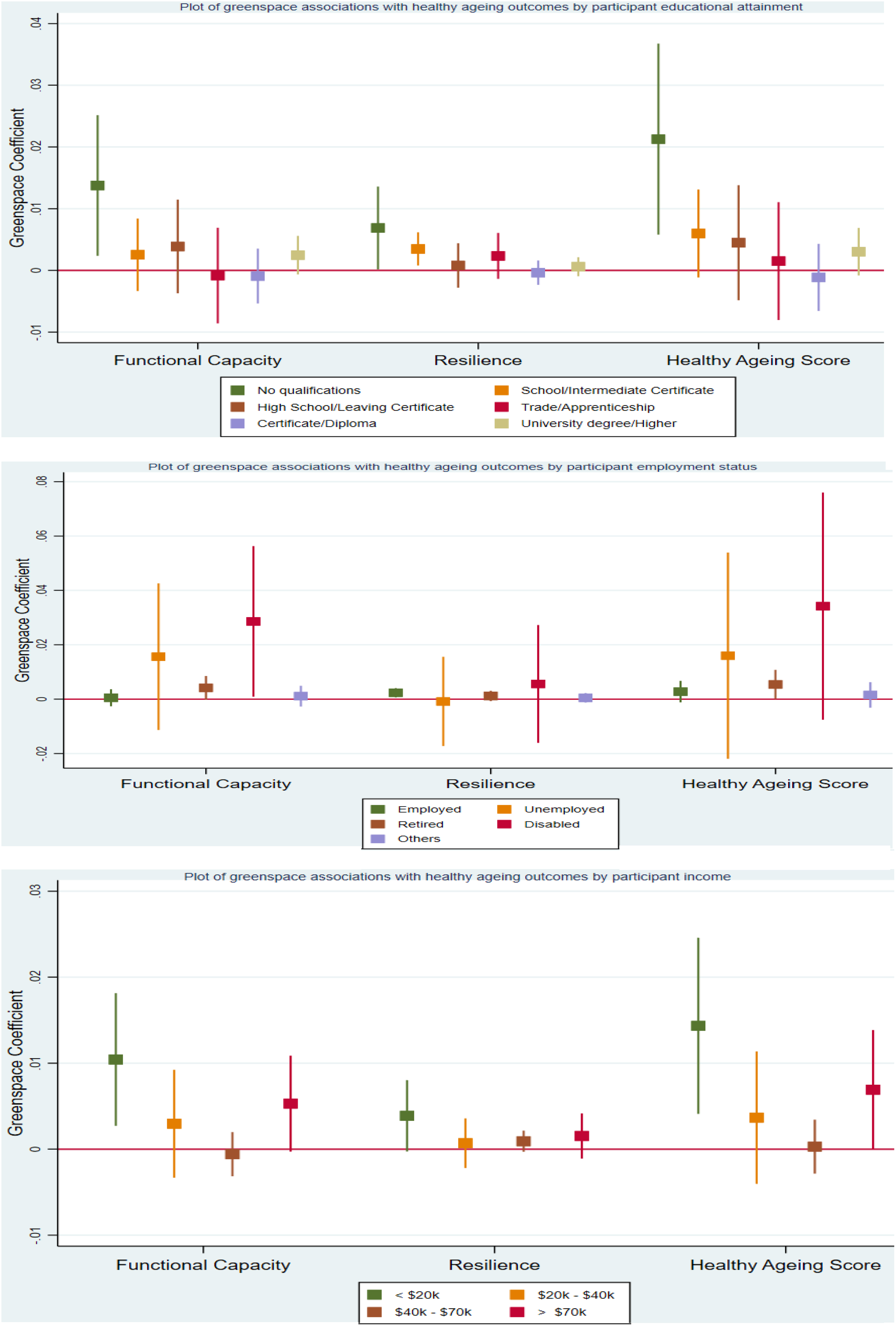Residing in a neighborhood with >30% tree canopy was most supportive of healthy ageing ( $β$ 0.47, 95% CI 0.37–0.57) and this significant positive association decreased slightly but remained significant after including interaction with academic qualification in the model ( $β$ 0.64, 95% CI 0.32–0.97) (Fig. 2).

Fig. 2.

Plot of green space associations with healthy ageing outcomes by participant socioeconomic status.

Likelihood ratio tests of the models with the interaction between green space and academic achievement versus the models without the interaction showed that the associations between resilience and %grass ( $χ^{2}$ 46.96, p 0.00); HAS and grass ( $χ^{2}$ 32.20, p 0.04); functional capacity and %tree canopy ( $χ^{2}$ 29.07, p 0.02); HAS and %tree canopy ( $χ^{2}$ 30.27, p 0.01) were significantly dependent on educational level. Grass levels of >30% appeared supportive of resilience except for school or intermediate certificate holders.

Tree canopy levels of 20–29% were no longer significant for functional capacity in the interaction model except for high school leavers. Also, tree canopy levels of 20–29% were no longer significant for the HAS in the interaction model except for high school leavers. The interaction plots in Figure 1 show unique functional capacity, resilience, and HAS trajectories for each level of educational attainment. The variation in the functional capacity, resilience, or HAS explainable by the distribution of grass, low-lying vegetation, or tree canopy across the statistical areas is negligible (Table 4 and Appendix).

Table 4.

Multilevel Linear Regression of the Associations Between Green Space Types and Healthy Ageing Domains and Effect Modification by Academic Achievement Controlling for Demographic and Socioeconomic Variables

GREEN SPACE VARIABLE	DEPENDENT VARIABLES			GREEN SPACE VARIABLE	DEPENDENT VARIABLES			GREEN SPACE VARIABLE	DEPENDENT VARIABLES
GREEN SPACE VARIABLE	FUNCTIONAL CAPACITY β (95% CI)	RESILIENCE β (95% CI)	HAS β (95% CI)	GREEN SPACE VARIABLE	FUNCTIONAL CAPACITY β (95% CI)	RESILIENCE β (95% CI)	HAS β (95% CI)	GREEN SPACE VARIABLE	FUNCTIONAL CAPACITY β (95% CI)	RESILIENCE β (95% CI)	HAS β (95% CI)
Interaction of % grass and academic qualification				Interaction of % low-lying vegetation and academic qualification				Interaction of % tree canopy and academic qualification
5 to 9#School/intermediate	−0.57 (−1.09 to −0.04)	−0.1 (−0.36 to 0.15)	−0.66 (−1.31 to −0.01)	5 to 9#School/intermediate	−0.04 (−0.2 to 0.12)	−0.1 (−0.18 to −0.02)	−0.14 (−0.34 to 0.06)	10 to 19#School/Intermediate	0.22 (−0.46 to 0.01)	−0.07 (−0.18 to 0.04)	−0.29 (−0.58 to −0.01)
5 to 9#High school/leaving	−0.39 (−0.92 to 0.14)	−0.28 (−0.54 to −0.03)	−0.66 (−1.31 to −0.01)	5 to 9#High school/leaving	−0.11 (−0.28 to 0.07)	−0.1 (−0.19 to −0.01)	−0.21 (−0.43 to 0.01)	10 to 19#High school/leaving	0.24 (−0.04 to 0.51)	−0.02 (−0.16 to 0.11)	0.21 (−0.13 to 0.55)
5 to 9#Trade/apprenticeship	−0.66 (−1.28 to −0.04)	−0.16 (−0.46 to 0.14)	−0.81 (−1.57 to −0.05)	5 to 9#Trade/apprenticeship	−0.05 (−0.23 to 0.13)	−0.06 (−0.15 to 0.03)	−0.11 (−0.34 to 0.11)	10 to 19#Trade/apprenticeship	0	−0.02 (−0.15 to 0.1)	−0.03 (−0.35 to 0.3)
5 to 9#Certificate/diploma	−0.46 (−0.95 to 0.02)	−0.13 (−0.36 to 0.11)	−0.58 (−1.18 to 0.01)	5 to 9#Certificate/diploma	−0.03 (−0.18 to 0.13)	−0.1 (−0.18 to −0.02)	−0.13 (−0.32 to 0.07)	10 to 19#Certificate/diploma	−0.02 (−0.25 to 0.21)	−0.06 (−0.17 to 0.06)	−0.07 (−0.36 to 0.21)
5 to 9#Universitydegree	−0.4 (−0.86 to 0.07)	−0.15 (−0.38 to 0.08)	−0.54 (−1.12 to 0.03)	5 to 9#University degree	−0.05 (−0.21 to 0.1)	−0.12 (−0.19 to −0.04)	−0.18 (−0.36 to 0.01)	10 to 19#University degree	−0.03 (−0.26 to 0.2)	−0.05 (−0.16 to 0.06)	−0.08 (−0.36 to 0.2)
10 to 19#School/intermediate	−0.42 (−0.95 to 0.11)	−0.04 (−0.3 to 0.22)	−0.45 (−1.11 to 0.2)	≥10#School/intermediate	−0.48 (−0.9 to −0.05)	−0.06 (−0.27 to 0.14)	−0.53 (−1.05 to −0.01)	20 to 29#School/intermediate	−0.04 (−0.32 to 0.23)	0.02 (−0.11 to 0.16)	−0.02 (−0.35 to 0.32)
10 to 19#High school/leaving	−0.26 (−0.8 to 0.27)	−0.22 (−0.48 to 0.04)	−0.48 (−1.14 to 0.18)	≥10#High school/leaving	−0.75 (−1.23 to −0.28)	−0.17 (−0.4 to 0.06)	−0.92 (−1.5 to −0.34)	20 to 29#High school/leaving	0.52 (0.21 to 0.83)	0.09 (−0.06 to 0.24)	0.61 (0.23 to 0.99)
10 to 19#Trade/apprenticeship	−0.61 (−1.23 to 0.01)	−0.08 (−0.39 to 0.22)	−0.69 (−1.45 to 0.08)	≥10#Trade/apprenticeship	−0.73 (−1.2 to −0.27)	−0.11 (−0.34 to 0.11)	−0.84 (−1.42 to −0.27)	20 to 29#Trade/apprenticeship	0.12 (−0.18 to 0.43)	0.02 (−0.13 to 0.17)	0.15 (−0.23 to 0.52)
10 to 19#Certificate/diploma	−0.3 (−0.79 to 0.18)	−0.06 (−0.3 to 0.18)	−0.36 (−0.96 to 0.24)	≥10#Certificate/diploma	−0.59 (−1 to −0.19)	−0.16 (−0.36 to 0.04)	−0.75 (−1.25 to −0.25)	20 to 29#Certificate/diploma	0.07 (−0.2 to 0.34)	0.01 (−0.12 to 0.14)	0.08 (−0.25 to 0.41)
10 to 19#University degree	−0.27 (−0.74 to 0.2)	−0.08 (−0.31 to 0.15)	−0.35 (−0.93 to 0.22)	≥10#University degree	−0.42 (−0.82 to −0.03)	−0.18 (−0.37 to 0.02)	−0.6 (−1.09 to −0.11)	20 to 29#University degree	0.07 (−0.19 to 0.34)	0.02 (−0.11 to 0.15)	0.1 (−0.23 to 0.42)
20 to 29#School/intermediate	−0.67 (−1.21 to −0.14)	−0.15 (−0.41 to 0.11)	−0.81 (−1.47 to −0.15)					≥30#School/intermediate	−0.13 (−0.43 to 0.18)	−0.11 (−0.26 to 0.04)	−0.23 (−0.61 to 0.14)
20 to 29#High school/leaving	−0.5 (−1.05 to 0.04)	−0.37 (−0.64 to −0.11)	−0.86 (−1.54 to −0.19)					≥30#High school/leaving	0.25 (−0.09 to 0.58)	−0.04 (−0.2 to 0.13)	0.21 (−0.21 to 0.63)
20 to 29#Trade/apprenticeship	−0.86 (−1.48 to −0.23)	−0.26 (−0.56 to 0.05)	−1.1 (−1.87 to −0.33)					≥30#Trade/apprenticeship	−0.07 (−0.41 to 0.27)	−0.05 (−0.22 to 0.11)	−0.12 (−0.54 to 0.3)
20 to 29#Certificate/diploma	−0.53 (−1.02 to −0.04)	−0.24 (−0.48 to 0)	−0.76 (−1.36 to −0.15)					≥30#Certificate/diploma	−0.08 (−0.38 to 0.22)	−0.12 (−0.26 to 0.03)	−0.19 (−0.56 to 0.17)
20 to 29#University degree	−0.43 (−0.91 to 0.05)	−0.27 (−0.51 to −0.04)	−0.7 (−1.29 to −0.11)					≥30#University degree	−0.12 (−0.42 to 0.17)	−0.12 (−0.27 to 0.02)	−0.24 (−0.61 to 0.12)
≥30#School/intermediate	−0.77 (−1.36 to −0.19)	−0.28 (−0.57 to 0)	−1.04 (−1.76 to −0.32)
≥30#High school/leaving	−0.91 (−1.54 to −0.28)	−0.5 (−0.81 to −0.19)	−1.4 (−2.18 to −0.62)
≥30#Trade/apprenticeship	−0.95 (−1.63 to −0.27)	−0.54 (−0.88 to −0.21)	−1.48 (−2.33 to −0.64)
≥30#Certificate/diploma	−0.67 (−1.21 to −0.12)	−0.38 (−0.64 to −0.11)	−1.03 (−1.7 to −0.36)
≥30#University degree	−0.54 (−1.07 to 0)	−0.34 (−0.61 to −0.08)	−0.88 (−1.54 to −0.21)
Green space variable				Green space variable				Green space variable
% Grass (ref: 0 to 4)				% Shrub (ref: 0 to 4)				% Tree (ref: 0 to 9)
5 to 9	0.33 (−0.12 to 0.79)	0.13 (−0.09 to 0.36)	0.47 (−0.09 to 1.02)	5 to 9	0.07 (−0.07 to 0.21)	0.11 (0.04 to 0.18)	0.18 (0.01 to 0.36)	10 to 19	0.18 (−0.01 to 0.36)	0.11 (0.02 to 0.2)	0.28 (0.05 to 0.51)
10 to 19	0.2 (−0.26 to 0.65)	0.06 (−0.16 to 0.28)	0.27 (−0.29 to 0.84)	≥10	0.52 (0.16 to 0.88)	0.18 (0 to 0.36)	0.69 (0.24 to 1.14)	20 to 29	0.18 (−0.05 to 0.4)	0.09 (−0.02 to 0.2)	0.25 (−0.03 to 0.53)
20 to 29	0.29 (−0.17 to 0.75)	0.2 (−0.03 to 0.42)	0.5 (−0.07 to 1.06)					≥30	0.42 (0.16 to 0.68)	0.24 (0.11 to 0.37)	0.64 (0.32 to 0.97)
≥30	0.35 (−0.15 to 0.85)	0.31 (0.07 to 0.56)	0.65 (0.04 to 1.27)
Participant characteristics				Participant characteristics				Participant characteristics
Gender (ref: male)				Gender (ref: male)				Gender (ref: male)
Female	−0.12 (−0.15 to −0.08)	0.05 (0.03 to 0.07)	−0.07 (−0.11 to −0.02)	Female	−0.12 (−0.15 to −0.08)	0.05 (0.03 to 0.07)	−0.07 (−0.11 to −0.02)	Female	−0.12 (−0.16 to −0.08)	0.05 (0.03 to 0.07)	−0.07 (−0.12 to −0.02)
Age group (ref: 45 to 54 years)				Age group (ref: 45 to 54 years)				Age group (ref: 45 to 54 years)
55 to 64	0	0.12 (0.09 to 0.14)	0.11 (0.06 to 0.17)	55 to 64	0	0.12 (0.09 to 0.14)	0.11 (0.06 to 0.17)	55 to 64	0	0.12 (0.09 to 0.14)	0.11 (0.06 to 0.17)
65 to 74	−0.09 (−0.15 to −0.03)	0.18 (0.15 to 0.21)	0.08 (0.01 to 0.15)	65 to 74	−0.09 (−0.15 to −0.03)	0.18 (0.15 to 0.2)	0.08 (0.01 to 0.16)	65 to 74	−0.1 (−0.16 to −0.04)	0.17 (0.14 to 0.2)	0.07 (0 to 0.14)
75+	−0.82 (−0.89 to −0.75)	0.06 (0.03 to 0.1)	−0.76 (−0.85 to −0.68)	75+	−0.81 (−0.89 to −0.74)	0.06 (0.03 to 0.1)	−0.76 (−0.85 to −0.67)	75+	−0.83 (−0.9 to −0.76)	0.06 (0.02 to 0.09)	−0.78 (−0.86 to −0.69)
Relationship status (ref: married/with partner)				Relationship status (ref: married/with partner)				Relationship status (ref: married/with partner)
Single	−0.12 (−0.19 to −0.04)	−0.07 (−0.11 to −0.04)	−0.19 (−0.28 to −0.1)	Single	−0.11 (−0.18 to −0.03)	−0.07 (−0.11 to −0.03)	−0.17 (−0.27 to −0.08)	Single	−0.1 (−0.18 to −0.03)	−0.07 (−0.11 to −0.03)	−0.17 (−0.26 to −0.08)
Widowed	−0.22 (−0.29 to −0.15)	−0.02 (−0.06 to 0.01)	−0.24 (−0.32 to −0.15)	Widowed	−0.21 (−0.28 to −0.14)	−0.02 (−0.06 to 0.01)	−0.24 (−0.32 to −0.15)	Widowed	−0.21 (−0.28 to −0.14)	−0.02 (−0.06 to 0.01)	−0.24 (−0.32 to −0.15)
Divorced	−0.1 (−0.17 to −0.03)	−0.05 (−0.08 to −0.02)	−0.15 (−0.23 to −0.07)	Divorced	−0.1 (−0.17 to −0.03)	−0.05 (−0.08 to −0.02)	−0.15 (−0.23 to −0.06)	Divorced	−0.09 (−0.16 to −0.02)	−0.05 (−0.08 to −0.01)	−0.14 (−0.22 to −0.06)
Separated	−0.27 (−0.39 to −0.15)	−0.14 (−0.2 to −0.08)	−0.41 (−0.55 to −0.26)	Separated	−0.27 (−0.38 to −0.15)	−0.14 (−0.2 to −0.08)	−0.4 (−0.55 to −0.26)	Separated	−0.26 (−0.37 to −0.14)	−0.14 (−0.2 to −0.08)	−0.4 (−0.54 to −0.25)
Employment status (ref: employed)				Employment status (ref: employed)				Employment status (ref: employed)
Unemployed	−0.52 (−0.68 to −0.36)	−0.21 (−0.29 to −0.13)	−0.73 (−0.93 to −0.53)	Unemployed	−0.51 (−0.67 to −0.35)	−0.21 (−0.29 to −0.13)	−0.72 (−0.92 to −0.52)	Unemployed	−0.51 (−0.67 to −0.35)	−0.21 (−0.29 to −0.14)	−0.72 (−0.92 to −0.52)
Retired	−0.28 (−0.34 to −0.22)	0.05 (0.02 to 0.08)	−0.23 (−0.3 to −0.15)	Retired	−0.28 (−0.34 to −0.22)	0.05 (0.02 to 0.08)	−0.23 (−0.3 to −0.15)	Retired	−0.28 (−0.34 to −0.22)	0.05 (0.02 to 0.08)	−0.23 (−0.3 to −0.16)
Disabled	−2.97 (−3.12 to −2.82)	−1.12 (−1.2 to −1.05)	−4.09 (−4.28 to −3.9)	Disabled	−2.98 (−3.13 to −2.83)	−1.12 (−1.2 to −1.05)	−4.1 (−4.28 to −3.91)	Disabled	−2.97 (−3.12 to −2.82)	−1.12 (−1.19 to −1.04)	−4.09 (−4.27 to −3.9)
Others	−0.14 (−0.19 to −0.1)	0.05 (0.02 to 0.07)	−0.1 (−0.16 to −0.04)	Others	−0.14 (−0.19 to −0.1)	0.05 (0.02 to 0.07)	−0.1 (−0.16 to −0.04)	Others	−0.15 (−0.2 to −0.1)	0.05 (0.02 to 0.07)	−0.1 (−0.16 to −0.04)
Income (ref: <$20k)				Income (ref: <$20k)				Income (ref: <$20k)
$20k to $40k	0.42 (0.35 to 0.49)	0.17 (0.13 to 0.2)	0.58 (0.5 to 0.66)	$20k to $40k	0.42 (0.36 to 0.49)	0.17 (0.13 to 0.2)	0.59 (0.5 to 0.67)	$20k to $40k	0.42 (0.35 to 0.48)	0.17 (0.13 to 0.2)	0.58 (0.5 to 0.66)
$40k to $70k	0.66 (0.59 to 0.72)	0.25 (0.22 to 0.28)	0.9 (0.82 to 0.97)	$40k to $70k	0.66 (0.6 to 0.73)	0.25 (0.22 to 0.28)	0.9 (0.83 to 0.98)	$40k to $70k	0.65 (0.58 to 0.71)	0.25 (0.22 to 0.28)	0.89 (0.81 to 0.96)
>$70k	0.51 (0.45 to 0.58)	0.18 (0.15 to 0.21)	0.68 (0.6 to 0.77)	>$70k	0.51 (0.45 to 0.58)	0.18 (0.15 to 0.21)	0.69 (0.61 to 0.77)	>$70k	0.5 (0.44 to 0.57)	0.17 (0.14 to 0.21)	0.67 (0.59 to 0.75)
Qualification (ref: no qualifications)				Qualification (ref: no qualifications)				Qualification (ref: no qualifications)
School/intermediate certificate	1.04 (0.53 to 1.55)	0.37 (0.12 to 0.62)	1.4 (0.77 to 2.02)	School/intermediate certificate	0.53 (0.4 to 0.65)	0.32 (0.25 to 0.38)	0.84 (0.68 to 0.99)	School/intermediate certificate	0.62 (0.41 to 0.82)	0.3 (0.2 to 0.4)	0.91 (0.66 to 1.16)
High school/leaving certificate	0.89 (0.38 to 1.39)	0.55 (0.31 to 0.8)	1.42 (0.8 to 2.05)	High school/leaving certificate	0.58 (0.44 to 0.71)	0.32 (0.26 to 0.39)	0.89 (0.72 to 1.05)	High school/leaving certificate	0.19 (−0.06 to 0.43)	0.24 (0.12 to 0.36)	0.43 (0.12 to 0.73)
Trade/apprenticeship	1.08 (0.48 to 1.68)	0.46 (0.17 to 0.75)	1.52 (0.78 to 2.26)	Trade/apprenticeship	0.43 (0.29 to 0.58)	0.31 (0.24 to 0.38)	0.74 (0.56 to 0.91)	Trade/apprenticeship	0.35 (0.12 to 0.59)	0.28 (0.17 to 0.4)	0.63 (0.35 to 0.92)
Certificate/diploma	0.98 (0.52 to 1.45)	0.42 (0.19 to 0.64)	1.38 (0.81 to 1.96)	Certificate/diploma	0.58 (0.46 to 0.7)	0.33 (0.27 to 0.39)	0.9 (0.75 to 1.05)	Certificate/diploma	0.54 (0.33 to 0.75)	0.3 (0.2 to 0.4)	0.84 (0.58 to 1.09)
University degree/higher	1.07 (0.62 to 1.51)	0.42 (0.2 to 0.64)	1.47 (0.92 to 2.03)	University degree/higher	0.74 (0.62 to 0.86)	0.32 (0.27 to 0.38)	1.05 (0.91 to 1.19)	University degree/higher	0.7 (0.49 to 0.9)	0.29 (0.18 to 0.39)	0.98 (0.73 to 1.23)
Random effects, variance (95% CI)				Random effects, variance (95% CI)				Random effects, variance (95% CI)
Level 2: statistical area 2	0.02 (0.01 to 0.03)	0.01 (0.00 to 0.01)	0.05 (0.04 to 0.07)	Level 2: statistical area 2	0.03 (0.02 to 0.04)	0.01 (0.00 to 0.01)	0.06 (0.04 to 0.08)	Level 2: statistical area 2	0.01 (0.01 to 0.02)	0.00 (0.00 to 0.01)	0.03 (0.02 to 0.04)
Level 1: participant	2.45 (2.41 to 2.49)	0.59 (0.58 to 0.60)	3.72 (3.70 to 3.78)	Level 1: participant	2.45 (2.41 to 2.49)	0.59 (0.58 to 0.60)	3.72, (3.66 to 3.78)	Level 1: participant	2.45 (2.41 to 2.49)	0.59 (0.58 to 0.60)	3.72 (3.66 to 3.78)
Intraclass correlation	0.01	0.01	0.01	Intraclass correlation	0.01	0.01	0.02	Intraclass correlation	0.01	0.00	0.01
Likelihood ratio test $χ^{2}$ (p)	24.75 (0.21)	46.96 (0.00)	32.20 (0.04)	Likelihood ratio test $χ^{2}$ (p)	15.62 (0.11)	14.51 (0.15)	15.93 (0.10)	Likelihood ratio test $χ^{2}$ (p)	31.80 (0.01)	11.76 (0.70)	30.27 (0.01)

# means interaction.

Bold: p < 0.05 (emboldened for green space and interaction variables only).

Discussion

Clearly, the pattern that increased lateral and vertical foliage is positively associated with healthy ageing benefits become obvious. An increasing percentage of tree cover by >30% was shown to be strongly significantly supportive of functional capacity, resilience, and overall healthy ageing. Conversely, increasing the percentage of grass appeared to be significantly detrimental to functional capacity, resilience, and overall HAS. Increasing low lying vegetation >10% was associated with increased functional capacity but not resilience or HAS. One possible explanation is that tree cover provides a great sense of immersion, and awe in nature while mitigating environmental stressors as participants engage in psychophysiological stress recovery and physical or social activity (Markevych et al., 2017). The pattern of the association of green space and HAS and its domains were seen to evolve from negative (grass) to mixed (low-lying vegetation) to positive (tree cover).

Our study has shown that the association and magnitude of benefit of green space exposure are not the same for people in different socioeconomic and educational groups. It also shows that exposure to different green space types can have a varied association with healthy ageing depending on individual socioeconomic circumstances. After controlling for other socioeconomic variables in the partitioned samples, low-income earners, partcipants with no qualifications, and the disabled appeared to benefit more from available green space.

The association between green space exposure and functional capacity, resilience, and HAS of participants earning <$20k was stronger and almost double that of participants earning >$70k. Similarly, after partitioning by educational attainment, the association between green space exposure and functional capacity, resilience, and HAS of participants with no academic qualifications was highest and approximately three times higher than that of participants with a university or higher degree. In terms of employment status, green space had the highest association with improved functional capacity for disabled people compared with employed, unemployed, or retired participants.

Increasing green space had a consistently positive association with functional capacity and resilience for single, married/with a partner and the widowed, and a consistently negative association with being divorced. Green space exposure had a deleterious influence on the functional capacity of the separated participants but appeared to improve their resilience. In addition, green space may provide them with psychological restoration and resilience to cope with their situation (Bell, Phoenix, Lovell, & Wheeler, 2014; Markevych et al., 2017; Schipperijn, Stigsdotter, Randrup, & Troelsen, 2010). Exposure to green space was shown to associate positively with the functional capacity of the employed, retired, and disabled but did not help the unemployed in terms of resilience. Increasing green space availability had a consistently positive association on the HAS and its dimensions for all income levels with the highest impact for groups earning <$20k ( $β$ 0.01, p 0.01).

Green space provision can be considered as one way of modifying the environment to promote health. The beneficial associations between green space and healthy ageing reported in this study is explainable by the mechanisms outlined in the general pathways outlined by Markevych et al. (2017). First, since deprived neighborhoods are least likely to be considered for protection from adverse environmental stressors such as air pollution, noise, and heat occasioned by industrial, commercial, or dense human activity (Ganzleben & Kazmierczak, 2020; World Health Organization, 2009), green spaces can act as an enclave to mitigate the effects of these environmental stressors. Second, people who are struggling and may live in densely populated areas or unsupportive households may wish to escape to the serenity of green spaces to recover.

This is especially relevant when such people cannot afford to move away or change their household composition. Third, green space encourages physical activity and is a setting for connection to self, making new social connections and strengthening existing ones. Given the reported green space associations with healthy ageing outcomes and large sample size in this study, the effect sizes are small, but this is expected, partly due to the large sample size and the theorized intermediary outcomes, activities, and behaviors that are the pathway activities that link green space and healthy ageing. We expect the effect sizes of green space with these intermediary outcomes and activities to be larger and more statistically significant but did not investigate that in this study. Therefore, policymakers should not mistake these findings to be irrelevant.

This analysis indicates that green space is an important resource that has the potential to support well-being, although differently, across socioeconomic groups. Although higher-income earners and graduates have more surrounding green space it is apparent that it does not necessarily translate to higher healthy ageing outcomes. This hints at the possibility of different socioeconomic groups engaging and benefiting differently from the available green space in their locality. Higher levels of green space have a disproportionately larger beneficial influence on disadvantaged groups and thereby help to reduce socioeconomic inequities in healthy ageing.

This finding can be linked to the “equigenesis” concept espoused by Rich Mitchell as a mechanism to narrow health inequality between advantaged and disadvantaged socioeconomic groups over time. He proposed that a mechanism to achieve “equigenesis” is by supporting the health and opportunities for the less advantaged group as much as, or perhaps even more than, the more advantaged group (Mitchell, 2013). It can be argued that wealthier people who may be already healthier can afford to live in greener places in pursuit of their active lifestyles unlike individuals earning <$20k with limited residential choices. We may never know the extent of benefits disadvantaged groups can derive from green spaces if wealth continues to be the determinant of access to such spaces.

It is possible also that the green space in some of the affluent neighborhoods, by design, serves mostly as an aesthetic to drive up property values ultimately resulting in outpricing lower-income earners from seeking residence in such neighborhoods. Studies have investigated connections between social determinants of health and cultural ecosystems that are derived from urban green space. Jennings, Larson, and Yun (2016) reported that the accessibility of local green space does not necessarily translate to health benefits if residents are unable to experience the cultural ecosystem services that urban green spaces provide (Jennings, Larson, Larson, & Yun, 2016).

Another explanation of the higher benefit of green space for low-income earners may be the trend toward larger houses on smaller lots with little or no suitable private outdoor green space for recreation compared with those of higher-income earners. Although all socioeconomic groups frequent green spaces to relax and socialize, lower-income earners rely heavily, if not absolutely, on their neighborhood green space for positive nature exposure specially to allow children to play more often than their higher-income counterparts (Wendel, Zarger, & Mihelcic, 2012). Therefore, providing more quality green space in disadvantaged areas can be a useful social policy to promote healthy ageing for the less advantaged, reducing disparity and equitable health outcomes for all.

Study limitations

As this is a cross-sectional study, the causative association of green space cannot be inferred. Also, since privately owned green space was not considered, there may be the possibility that health benefits from private green space are indistinguishable from publicly accessible green space, but this study cannot ascertain. The quality (including facilities), individual preferences for green space features, and safety within and around the green space were not taken into consideration in our model. The issues of residential self-selection, relocation, and mobility could also confound the findings, yet are not considered in this study.

It is also possible that the participants could have moved residences and their healthy ageing profiles may not be associated with their present surrounding green space. There is a high potential that economically disadvantaged participants with worse HAS profiles move to less green areas and economically advantaged participants with healthier ageing profiles relocate to leafier areas. Further research will investigate the role of residential self-selection in modifying the green space and healthy ageing relationship.

In conclusion, these findings show that a combination of grass, low-lying vegetation, and tree canopy of not <30% each in publicly accessible green space is a crucial public health resource, especially for the low-income retired population. Investment in green space infrastructure in areas where low-income earners and retirees live is a step in the direction of equity and enforcement of environmental justice and healthy ageing. From a policy perspective, it is beneficial to involve these groups in green space planning to understand how best green spaces can be designed to best support their engagement with such spaces.

Our finding supports decisions to invest more public and if possible, corporate and private resources into greening disadvantaged neighborhoods for the benefit of all. Further research is required to understand how and why individuals in different socioeconomic and demographic groups and life stages engage with or utilize the different features and types of green spaces available to them. Also, further research must investigate if the influence of surrounding green space is dependent on whether it is fragmented or in a single piece (Shen & Lung, 2018; Wen, Albert, & Von Haaren, 2020).

Acknowledgments

This research was completed using data collected through the 45 and Up Study (http://www.saxinstitute.org.au). The 45 and Up Study is managed by the Sax Institute in collaboration with major partner Cancer Council New South Wales (NSW) and partners the National Heart Foundation of Australia (NSW Division), NSW Ministry of Health, NSW Government Family & Community Services–Ageing, Carers, and the Disability Council NSW, and the Australian Red Cross Blood Service. We also thank the Secure Unified Research Environment (SURE) team for providing us access to the data and a secure analysis platform. We thank the many thousands of people for participating in the 45 and Up Study. We are grateful to the National Ageing Research Institute for its work on developing the Healthy Ageing Quiz.

Authors' Contributions

Conceptualization, investigation, methodology, visualization, analysis, and writing—original draft preparation by E.E.J. Conceptualization, funding acquisition, methodology, supervision, validation, methodology, and writing—reviewing and editing by T.A.-B. Conceptualization, funding acquisition, supervision, validation, methodology, and writing—reviewing and editing by X.F. Conceptualization, supervision, validation, methodology, and writing—reviewing and editing by P.Y. and C.B.-H.

Footnotes

Ethical statements

The conduct of the 45 and Up Study was approved by the University of New South Wales Human Research Ethics Committee (HREC), the University of Wollongong, and ISLHD Health and Medical Human Research Ethics Committee, and the UOW Social Sciences Human Research Ethics Committee approved this project (ethics no. 2016/158, 2020/206).

Author Disclosure Statement

No competing financial interests exist.

Funding Information

This project received funding from Hort Innovation Limited with co-investment from the University of Wollongong (UOW) Faculty of Social Sciences, the UOW Global Challenges initiative, and the Australian Government (project no. GC15005). X.F.'s contribution to this project was also supported by a National Health and Medical Research Council Career Development Fellowship (no. 1148792). X.F. and T.A.-B. are also supported by a National Health and Medical Research Council project grant (no. 1101065). T.A.-B. is supported by a National Health and Medical Research Council Boosting Dementia Research Leader Fellowship (no. 1140317). The study design, analysis, interpretation of the data, writing the report, and decision to submit the report for publication are of the authors only.

Appendix.

Multilevel Linear Regression of the Associations Between Green Space Types and Healthy Ageing Domains and Effect Modification by Academic Achievement with Controls for Demographic and Socioeconomic Variables

GREEN SPACE VARIABLE	DEPENDENT VARIABLES			GREEN SPACE VARIABLE	DEPENDENT VARIABLES			GREEN SPACE VARIABLE	DEPENDENT VARIABLES
GREEN SPACE VARIABLE	FUNCTIONAL CAPACITY β (95% CI)	RESILIENCE β (95% CI)	HAS β (95% CI)	GREEN SPACE VARIABLE	FUNCTIONAL CAPACITY β (95% CI)	RESILIENCE β (95% CI)	HAS β (95% CI)	GREEN SPACE VARIABLE	FUNCTIONAL CAPACITY β (95% CI)	RESILIENCE β (95% CI)	HAS β (95% CI)
Interaction of % grass and academic qualification				Interaction of % low-lying vegetation and academic qualification				Interaction of % tree canopy and academic qualification
5 to 9#School/intermediate	−0.45 (−0.98 to 0.07)	−0.06 (−0.31 to 0.2)	−0.5 (−1.15 to 0.14)	5 to 9#School/intermediate	−0.06 (−0.22 to 0.1)	−0.11 (−0.19 to −0.03)	−0.17 (−0.37 to 0.02)	10 to 19#School/intermediate	0.22 (−0.45 to 0.01)	−0.07 (−0.18 to 0.04)	−0.29 (−0.57 to −0.01)
5 to 9#High school/leaving	−0.33 (−0.85 to 0.19)	−0.26 (−0.52 to −0.01)	−0.58 (−1.23 to 0.06)	5 to 9#High school/leaving	−0.11 (−0.28 to 0.07)	−0.11 (−0.19 to −0.02)	−0.22 (−0.44 to 0)	10 to 19#High school/leaving	0.21 (−0.06 to 0.49)	−0.01 (−0.15 to 0.12)	0.2 (−0.14 to 0.53)
5 to 9#Trade/apprenticeship	−0.53 (−1.14 to 0.07)	−0.13 (−0.43 to 0.17)	−0.66 (−1.4 to 0.09)	5 to 9#Trade/apprenticeship	−0.07 (−0.25 to 0.11)	−0.08 (−0.17 to 0.01)	−0.15 (−0.37 to 0.07)	10 to 19#Trade/apprenticeship	−0.04 (−0.3 to 0.22)	−0.03 (−0.16 to 0.1)	−0.07 (−0.39 to 0.25)
5 to 9#Certificate/diploma	−0.4 (−0.88 to 0.08)	−0.1 (−0.34 to 0.13)	−0.49 (−1.09 to 0.1)	5 to 9#Certificate/diploma	−0.03 (−0.18 to 0.13)	−0.12 (−0.19 to −0.04)	−0.15 (−0.34 to 0.04)	10 to 19#Certificate/diploma	−0.03 (−0.26 to 0.2)	−0.04 (−0.16 to 0.07)	−0.08 (−0.36 to 0.21)
5 to 9#University degree	−0.32 (−0.78 to 0.15)	−0.12 (−0.35 to 0.1)	−0.44 (−1.01 to 0.13)	5 to 9#University degree	−0.06 (−0.21 to 0.09)	−0.13 (−0.2 to −0.06)	−0.19 (−0.37 to −0.01)	10 to 19#University degree	−0.4 (−0.26 to 0.19)	−0.03 (−0.14 to 0.08)	−0.08 (−0.35 to 0.2)
10 to 19#School/intermediate	−0.35 (−0.88 to 0.17)	−0.01 (−0.26 to 0.25)	−0.35 (−1 to 0.3)	≥10#School/intermediate	−0.41 (−0.81 to −0.01)	−0.09 (−0.29 to 0.1)	−0.5 (−0.99 to 0)	20 to 29#School/intermediate	−0.5 (−0.32 to 0.22)	0.02 (−0.11 to 0.15)	−0.03 (−0.36 to 0.3)
10 to 19#High school/leaving	−0.27 (−0.8 to 0.26)	−0.21 (−0.47 to 0.04)	−0.48 (−1.13 to 0.17)	≥10#High school/leaving	−0.65 (−1.11 to −0.2)	−0.19 (−0.41 to 0.03)	−0.84 (−1.41 to −0.28)	20 to 29#High school/leaving	0.48 (0.17 to 0.79)	0.09 (−0.06 to 0.24)	0.57 (0.19 to 0.94)
10 to 19#Trade/apprenticeship	−0.53 (−1.13 to 0.08)	−0.08 (−0.37 to 0.22)	−0.6 (−1.35 to 0.16)	≥10#Trade/apprenticeship	−0.64 (−1.09 to −0.19)	−0.13 (−0.35 to 0.09)	−0.76 (−1.32 to −0.21)	20 to 29#Trade/apprenticeship	0.09 (−0.21 to 0.39)	0.02 (−0.13 to 0.17)	0.11 (−0.26 to 0.48)
10 to 19#Certificate/diploma	−0.29 (−0.77 to 0.2)	−0.04 (−0.28 to 0.19)	−0.33 (−0.92 to 0.27)	≥10#Certificate/diploma	−0.51 (−0.9 to −0.12)	−0.17 (−0.36 to 0.02)	−0.67 (−1.15 to −0.19)	20 to 29#Certificate/diploma	0.46 (−0.22 to 0.31)	0.01 (−0.12 to 0.14)	0.06 (−0.27 to 0.38)
10 to 19#University degree	−0.24 (−0.71 to 0.22)	−0.07 (−0.29 to 0.16)	−0.31 (−0.89 to 0.26)	≥10#University degree	−0.34 (−0.72 to 0.04)	−0.2 (−0.39 to −0.01)	−0.54 (−1.01 to −0.07)	20 to 29#University degree	0.06 (−0.2 to 0.32)	0.04 (−0.09 to 0.16)	0.09 (−0.23 to 0.41)
20 to 29#School/intermediate	−0.58 (−1.11 to −0.06)	−0.12 (−0.38 to 0.14)	−0.69 (−1.34 to −0.04)					≥30#School/intermediate	−0.15 (−0.45 to 0.15)	−0.13 (−0.27 to 0.02)	−0.27 (−0.64 to 0.1)
20 to 29#High school/leaving	−0.51 (−1.05 to 0.02)	−0.37 (−0.64 to −0.11)	−0.87 (−1.54 to −0.21)					≥30#High school/leaving	0.2 (0.13 to 0.53)	−0.04 (−0.21 to 0.12)	0.16 (−0.25 to 0.57)
20 to 29#Trade/apprenticeship	−0.75 (−1.36 to −0.14)	−0.24 (−0.54 to 0.06)	−0.98 (−1.74 to −0.23)					≥30#Trade/apprenticeship	−0.1 (−0.43 to 0.24)	−0.06 (−0.22 to 0.1)	−0.15 (−0.57 to 0.26)
20 to 29#Certificate/diploma	−0.49 (−0.98 to 0)	−0.22 (−0.46 to 0.02)	−0.7 (−1.3 to −0.1)					≥30#Certificate/diploma	−0.11 (−0.4 to 0.19)	−0.13 (−0.27 to 0.02)	−0.23 (−0.59 to 0.14)
20 to 29#University degree	−0.38 (−0.85 to 0.09)	−0.26 (−0.49 to −0.03)	−0.63 (−1.22 to −0.05)					≥30#University degree	−0.15 (−0.44 to 0.14)	−0.12 (−0.26 to 0.03)	−0.26 (−0.62 to 0.1)
≥30#School/intermediate	−0.6 (−1.18 to −0.02)	−0.21 (−0.49 to 0.07)	−0.79 (−1.51 to −0.08)
≥30#High school/leaving	−0.79 (−1.42 to −0.17)	−0.47 (−0.78 to −0.17)	−1.25 (−2.02 to −0.48)
≥30#Trade/apprenticeship	−0.78 (−1.46 to −0.11)	−0.49 (−0.82 to −0.16)	−1.26 (−2.09 to −0.43)
≥30#Certificate/diploma	−0.57 (−1.11 to −0.03)	−0.33 (−0.6 to −0.07)	−0.89 (−1.56 to −0.22)
≥30#University degree	−0.41 (−0.95 to 0.12)	−0.31 (−0.57 to −0.04)	−0.71 (−1.37 to −0.05)
Green space variable				Green space variable				Green space variable
% Grass (ref: 0 to 4)				%Shrub (ref: 0 to 4)				%Tree (ref: 0 to 9)
5 to 9	0.26 (−0.19 to 0.71)	0.11 (−0.11 to 0.33)	0.36 (−0.19 to 0.92)	5 to 9	0.07 (−0.07 to 0.21)	0.13 (0.06 to 0.19)	0.2 (0.03 to 0.37)	10 to 19	0.19 (0.01 to 0.37)	0.1 (0.01 to 0.19)	0.28 (0.06 to 0.51)
10 to 19	0.17 (−0.29 to 0.62)	0.05 (−0.17 to 0.27)	0.24 (−0.32 to 0.79)	≥10	0.45 (0.11 to 0.79)	0.2 (0.03 to 0.36)	0.64 (0.22 to 1.06)	20 to 29	0.19 (−0.03 to 0.41)	0.08 (−0.03 to 0.19)	0.25 (−0.02 to 0.53)
20 to 29	0.24 (−0.22 to 0.69)	0.19 (−0.04 to 0.41)	0.44 (−0.12 to 1)					≥30	0.45 (0.19 to 0.71)	0.24 (0.11 to 0.36)	0.67 (0.35 to 0.99)
≥30	0.23 (−0.26 to 0.73)	0.28 (0.03 to 0.52)	0.5 (−0.11 to 1.11)
Participant characteristics				Participant characteristics				Participant characteristics
Gender (ref: male)				Gender (ref: male)				Gender (ref: male)
Female	−0.12 (−0.16 to −0.08)	0.05 (0.03 to 0.07)	−0.07 (−0.12 to −0.02)	Female	−0.12 (−0.16 to −0.08)	0.05 (0.03 to 0.07)	−0.07 (−0.12 to −0.02)	Female	−0.12 (−0.16 to 0.09)	0.05 (0.03 to 0.07)	−0.07 (−0.12 to −0.03)
Age group (ref: 45 to 54 years)				Age group (ref: 45 to 54 years)				Age group (ref: 45 to 54 years)
55 to 64	0 (−0.05 to 0.04)	0.11 (0.09 to 0.14)	0.11 (0.05 to 0.16)	55 to 64	0 (−0.05 to 0.04)	0.11 (0.09 to 0.14)	0.11 (0.06 to 0.17)	55 to 64	0 (−0.05 to 0.04)	0.11 (0.09 to 0.14)	0.11 (0.05 to 0.16)
65 to 74	−0.1 (−0.16 to −0.04)	0.17 (0.14 to 0.2)	0.06 (−0.01 to 0.14)	65 to 74	−0.1 (−0.16 to −0.04)	0.17 (0.14 to 0.2)	0.06 (−0.01 to 0.14)	65 to 74	−0.11 (−0.17 to −0.05)	0.16 (0.13 to 0.19)	0.05 (−0.02 to 0.13)
75+	−0.84 (−0.91 to −0.77)	0.05 (0.01 to 0.08)	−0.8 (−0.89 to −0.71)	75+	−0.83 (−0.91 to −0.76)	0.05 (0.02 to 0.09)	−0.79 (−0.88 to −0.7)	75+	−0.85 (−0.92 to −0.78)	0.04 (0.01 to 0.08)	−0.81 (−0.9 to −0.72)
Relationship status (ref: married/with partner)				Relationship status (ref: married/with partner)				Relationship status (ref: married/with partner)
Single	−0.13 (−0.2 to −0.05)	−0.07 (−0.11 to −0.04)	−0.19 (−0.29 to −0.1)	Single	−0.11 (−0.19 to −0.04)	−0.07 (−0.11 to −0.03)	−0.18 (−0.27 to −0.09)	Single	−0.11 (−0.18 to −0.03)	−0.07 (−0.11 to −0.03)	−0.18 (−0.27 to −0.09)
Widowed	−0.21 (−0.28 to −0.14)	−0.02 (−0.05 to 0.01)	−0.23 (−0.31 to −0.15)	Widowed	−0.21 (−0.28 to −0.14)	−0.02 (−0.06 to 0.01)	−0.23 (−0.31 to −0.15)	Widowed	−0.2 (−0.27 to −0.14)	−0.02 (−0.06 to 0.01)	−0.23 (−0.31 to −0.14)
Divorced	−0.11 (−0.17 to −0.04)	−0.05 (−0.08 to −0.02)	−0.16 (−0.24 to −0.07)	Divorced	−0.1 (−0.17 to −0.04)	−0.05 (−0.08 to −0.02)	−0.15 (−0.24 to −0.07)	Divorced	−0.1 (−0.17 to −0.03)	−0.05 (−0.08 to −0.01)	−0.15 (−0.23 to −0.06)
Separated	−0.28 (−0.39 to −0.16)	−0.14 (−0.19 to −0.08)	−0.41 (−0.55 to −0.27)	Separated	−0.27 (−0.39 to −0.16)	−0.14 (−0.19 to −0.08)	−0.41 (−0.55 to −0.26)	Separated	−0.26 (−0.38 to −0.15)	−0.13 (−0.19 to −0.08)	−0.4 (−0.54 to −0.26)
Employment status (ref: employed)				Employment status (ref: employed)				Employment status (ref: employed)
Unemployed	−0.54 (−0.7 to −0.39)	−0.22 (−0.3 to −0.15)	−0.76 (−0.96 to −0.57)	Unemployed	−0.54 (−0.7 to −0.38)	−0.22 (−0.3 to −0.15)	−0.76 (−0.95 to −0.56)	Unemployed	−0.53 (−0.69 to −0.37)	−0.23 (−0.3 to −0.15)	−0.76 (−0.95 to −0.56)
Retired	−0.27 (−0.33 to −0.21)	0.06 (0.03 to 0.09)	−0.22 (−0.29 to −0.14)	Retired	−0.27 (−0.33 to −0.21)	0.06 (0.03 to 0.09)	−0.22 (−0.29 to −0.14)	Retired	−0.28 (−0.33 to −0.22)	0.06 (0.03 to 0.09)	−0.22 (−0.29 to −0.15)
Disabled	−2.96 (−3.11 to −2.81)	−1.11 (−1.18 to −1.04)	−4.07 (−4.25 to −3.88)	Disabled	−2.97 (−3.11 to −2.82)	−1.11 (−1.18 to −1.04)	−4.07 (−4.26 to −3.89)	Disabled	−2.96 (−3.11 to −2.81)	−1.11 (−1.18 to −1.03)	−4.06 (−4.25 to −3.88)
Volunteer	−0.12 (−0.22 to −0.01)	0.1 (0.04 to 0.15)	−0.02 (−0.16 to 0.11)	Volunteer	−0.12 (−0.22 to −0.01)	0.1 (0.04 to 0.15)	−0.02 (−0.16 to 0.11)	Volunteer	−0.12 (−0.23 to −0.01)	0.1 (0.04 to 0.15)	−0.03 (−0.16 to 0.1)
Others	−0.14 (−0.19 to −0.09)	0.04 (0.02 to 0.07)	−0.1 (−0.16 to −0.04)	Others	−0.14 (−0.19 to −0.09)	0.04 (0.02 to 0.07)	−0.1 (−0.16 to −0.04)	Others	−0.15 (−0.19 to −0.1)	0.04 (0.02 to 0.07)	−0.11 (−0.16 to −0.05)
Income (ref: < $20k)				Income (ref: <$20k)				Income (ref: <$20k)
Other/undisclosed	0.3 (0.17 to 0.43)	0.14 (0.08 to 0.2)	0.44 (0.28 to 0.6)	Other/undisclosed	0.3 (0.17 to 0.43)	0.14 (0.07 to 0.2)	0.44 (0.27 to 0.6)	Other/undisclosed	0.3 (0.17 to 0.43)	0.14 (0.07 to 0.2)	0.43 (0.27 to 0.6)
$20k to $40k	0.41 (0.35 to 0.48)	0.16 (0.13 to 0.19)	0.57 (0.49 to 0.65)	$20k to $40k	0.42 (0.35 to 0.48)	0.16 (0.13 to 0.19)	0.57 (0.49 to 0.65)	$20k to $40k	0.41 (0.34 to 0.47)	0.16 (0.13 to 0.19)	0.57 (0.49 to 0.65)
$40k to $70k	0.65 (0.59 to 0.71)	0.25 (0.22 to 0.28)	0.89 (0.81 to 0.96)	$40k to $70k	0.65 (0.59 to 0.72)	0.25 (0.22 to 0.28)	0.89 (0.81 to 0.97)	$40k to $70k	0.64 (0.57 to 0.7)	0.24 (0.21 to 0.27)	0.88 (0.8 to 0.95)
>$70k	0.5 (0.44 to 0.57)	0.18 (0.15 to 0.21)	0.67 (0.59 to 0.75)	>$70k	0.51 (0.44 to 0.57)	0.18 (0.15 to 0.21)	0.68 (0.6 to 0.76)	>$70k	0.49 (0.43 to 0.56)	0.17 (0.14 to 0.2)	0.66 (0.58 to 0.74)
Qualification (ref: no qualifications)				Qualification (ref: no qualifications)				Qualification (ref: no qualifications)
School/intermediate certificate	0.94 (0.43 to 1.44)	0.33 (0.08 to 0.58)	1.25 (0.62 to 1.87)	School/intermediate certificate	0.53 (0.41 to 0.65)	0.32 (0.26 to 0.38)	0.84 (0.69 to 0.99)	School/intermediate certificate	0.61 (0.41 to 0.81)	0.3 (0.2 to 0.4)	0.91 (0.66 to 1.15)
High school/leaving certificate	0.85 (0.35 to 1.35)	0.54 (0.29 to 0.78)	1.37 (0.75 to 1.99)	High school/leaving certificate	0.57 (0.44 to 0.7)	0.32 (0.26 to 0.39)	0.88 (0.72 to 1.04)	High school/leaving certificate	0.21 (−0.03 to 0.45)	0.23 (0.12 to 0.35)	0.44 (0.14 to 0.74)
Trade/apprenticeship	0.97 (0.38 to 1.55)	0.44 (0.15 to 0.72)	1.38 (0.66 to 2.11)	Trade/apprenticeship	0.44 (0.3 to 0.58)	0.32 (0.25 to 0.38)	0.75 (0.58 to 0.92)	Trade/apprenticeship	0.38 (0.15 to 0.61)	0.28 (0.17 to 0.39)	0.66 (0.38 to 0.94)
Certificate/diploma	0.93 (0.47 to 1.4)	0.39 (0.16 to 0.62)	1.31 (0.73 to 1.88)	Certificate/diploma	0.58 (0.46 to 0.7)	0.33 (0.27 to 0.39)	0.9 (0.75 to 1.04)	Certificate/diploma	0.55 (0.35 to 0.75)	0.3 (0.2 to 0.4)	0.84 (0.59 to 1.09)
University degree/higher	1 (0.56 to 1.45)	0.4 (0.18 to 0.62)	1.39 (0.84 to 1.94)	University degree/higher	0.73 (0.62 to 0.85)	0.33 (0.27 to 0.38)	1.05 (0.91 to 1.19)	University degree/higher	0.71 (0.5 to 0.91)	0.27 (0.17 to 0.37)	0.97 (0.72 to 1.22)
Random effects, variance (95% CI)				Random effects, variance (95% CI)				Random effects, variance (95% CI)
Level 2: statistical area 2	0.02 (0.02 to 0.03)	0.006 (0.00 to 0.009)	0.05 (0.04 to 0.08)	Level 2: statistical area 2	0.03 (0.02 to 0.04)	0.01 (0.004 to 0.009)	0.06 (0.05 to 0.08)	Level 2: statistical area 2	0.013 (0.01 to 0.02)	0.00 (0.00 to 0.01)	0.03 (0.02 to 0.04)
Level 1: participant	2.47 (2.43 to 2.51)	0.59 (0.58 to 0.60)	3.76 (3.70 to 3.810)	Level 1: participant	2.47 (2.43 to 2.51)	0.59 (0.58 to 0.60)	3.76, (3.70 to 3.81)	Level 1: participant	2.47 (2.43 to 2.51)	0.59 (0.58 to 0.60)	3.76 (3.70 to 3.82)
Intraclass correlation	0.01	0.01	0.01	Intraclass correlation	0.01	0.01	0.02	Intraclass correlation	0.01	0.00	0.01
Likelihood ratio test	20.70 (0.42)	43.78 (0.00)	27.81 (0.11)	Likelihood ratio test	13.53 (0.20)	16.95 (0.08)	14.53 (0.15)	Likelihood ratio test	29.07 (0.02)	12.54 (0.64)	28.43 (0.02)

# means interaction.

Bold: p < 0.05 (emboldened for green space and interaction variables only).

References

45 and Up Study Collaborators et al. (2008). Cohort profile: The 45 and up study. International Journal of Epidemiology, 37, 941–947.

Australian Bureau of Statistics (2016). 1270.0.55.001 - Australian Statistical Geography Standard (ASGS): Volume 1 - Main structure and greater capital city statistical areas, July 2016. Canberra: Australian Bureau of Statistics.

Astell-Burt

, & Feng

(2019). Association of urban green space with mental health and general health among adults in Australia. JAMA Network Open, 2, e198209–e198209.

Astell-Burt

, Feng

, & Kolt

G. S.

(2014). Is neighborhood green space associated with a lower risk of type 2 diabetes? Evidence from 267,072 Australians. Diabetes Care, 37, 197–201.

Astell-Burt

, Mitchell

, & Hartig

(2014). The association between green space and mental health varies across the lifecourse. A longitudinal study. Journal of Epidemiology and Community Health, 68, 578–583.

Astell-Burt

, Navakatikyan

M. A.

, & Feng

(2020). Urban green space, tree canopy and 11-year risk of dementia in a cohort of 109,688 Australians. Environment International, 145, 106102.

Bartram

(2021). Age and life satisfaction: Getting control variables under control. Sociology, 55, 421–437.

Beard

J. R.

, Officer

, De Carvalho

I. A.

, Sadana

, Pot

A. M.

, Michel

J.-P.

, Lloyd-Sherlock

, Epping-Jordan

J. E.

, Peeters

G. G.

, & Mahanani

W. R.

(2016). The World report on ageing and health: A policy framework for healthy ageing. The Lancet, 387, 2145–2154.

Bell

S. L.

, Phoenix

, Lovell

. and Wheeler

B. W.

(2014). Green space, health and well-being: Making space for individual agency. Health and Place, 30, 287–292.

10.

Braveman

, Arkin

, Orleans

, Proctor

, & Plough

(2017). What is health equity? And what difference does a definition make? Princeton, NJ: Robert Wood Johnson Foundation report.

11.

Brown

S. C.

, Lombard

, Wang

, Byrne

M. M.

, Toro

, Plater-Zyberk

, Feaster

D. J.

, Kardys

, Nardi

M. I.

, & Perez-Gomez

(2016). Neighborhood greenness and chronic health conditions in Medicare beneficiaries. American Journal of Preventive Medicine, 51, 78–89.

12.

Brown

S. C.

, Perrino

, Lombard

, Wang

, Toro

, Rundek

, Gutierrez

C. M.

, Dong

, Plater-Zyberk

, & Nardi

M. I.

(2018). Health disparities in the relationship of neighborhood greenness to mental health outcomes in 249,405 US Medicare beneficiaries. International Journal of Environmental Research and Public Health, 15, 430.

13.

Cherrie

M. P.

, Shortt

N. K.

, Mitchell

R. J.

, Taylor

A. M.

, Redmond

, Thompson

C. W.

, Starr

J. M.

, Deary

I. J.

, & Pearce

J. R.

(2018). Green space and cognitive ageing: A retrospective life course analysis in the Lothian Birth Cohort 1936. Social Science & Medicine, 196, 56–65.

14.

Clarke

, & Nieuwenhuijsen

E. R.

(2009). Environments for healthy ageing: A critical review. Maturitas, 64, 14–19.

15.

de Keijzer

, Bauwelinck

, & Dadvand

(2020). Long-term exposure to residential greenspace and healthy ageing: A systematic review. Current Environmental Health Reports, 7, 65–88.

16.

de Keijzer

, Tonne

, Sabia

, Basagaña

, Valentín

, Singh-Manoux

, Antó

J. M.

, Alonso

, Nieuwenhuijsen

M. J.

, & Sunyer

(2019). Green and blue spaces and physical functioning in older adults: Longitudinal analyses of the Whitehall II study. Environment International, 122, 346–356.

17.

Department of Education

a. e. (2019). Benefits of educational attainment. Canberra, Australia: S. a. e. Australian Government Department of Education.

18.

Ekkel

E. D.

, & de Vries

(2017). Nearby green space and human health: Evaluating accessibility metrics. Landscape and Urban Planning, 157, 214–220.

19.

Feng

, Toms

, & Astell-Burt

(2021). Association between green space, outdoor leisure time and physical activity. Urban Forestry & Urban Greening, 66, 127349.

20.

Frumkin

(2001). Beyond toxicity: Human health and the natural environment. American Journal of Preventive Medicine, 20, 234–240.

21.

Ganzleben

, & Kazmierczak

(2020). Leaving no one behind–understanding environmental inequality in Europe. Environmental Health, 19, 1–7.

22.

Gong

, Gallacher

, Palmer

, & Fone

(2014). Neighbourhood green space, physical function and participation in physical activities among elderly men: The Caerphilly Prospective study. International Journal of Behavioral Nutrition and Physical Activity, 11, 40.

23.

Hartig

, Mitchell

, De Vries

, & Frumkin

(2014). Nature and health. Annual Review of Public Health, 35, 207–228.

24.

Jennings

, Baptiste

A. K.

, Jelks

, & Skeete

(2017). Urban green space and the pursuit of health equity in parts of the United States. International Journal of Environmental Research and Public Health, 14, 1432.

25.

Jennings

, Larson

, & Yun

(2016). Advancing sustainability through urban green space: Cultural ecosystem services, equity, and social determinants of health. International Journal of Environmental Research and Public Health, 13, 196.

26.

John

E. E.

, Astell-Burt

, Yu

, Brennan-Horley

, & Feng

(2021). Development of a composite healthy ageing score: Evidence from middle-to-older aged Australians. Wollongong, Australia: University of Wollongong.

27.

Kling

H. E.

(2018). The effect of a park-based physical activity program on cardiovascular, strength, and mobility outcomes among a sample of racially/ethnically diverse adults aged 55 or older. Preventing Chronic Disease, 15, E166.

28.

Lachowycz

, & Jones

A. P.

(2014). Does walking explain associations between access to greenspace and lower mortality?. Social Science & Medicine, 107, 9–17.

29.

Leigh

(2008). Returns to education in Australia. Economic Papers: A Journal of Applied Economics and Policy, 27, 233–249.

30.

Leigh

, & Ryan

(2005). Estimating returns to education: Three natural experiment techniques compared. DISCUSSION PAPER NO. 493, Centre for Economic Policy Research, The Australian National University, Canberra.

31.

Lin

B. B.

, Fuller

R. A.

, Bush

, Gaston

K. J.

, & Shanahan

D. F.

(2014). Opportunity or orientation? Who uses urban parks and why. PLoS One, 9, e87422.

32.

Maas

, Verheij

R. A.

, de Vries

, Spreeuwenberg

, Schellevis

F. G.

, & Groenewegen

P. P.

(2009). Morbidity is related to a green living environment. Journal of Epidemiology and Community Health, 63, 967–973.

33.

Markevych

, Schoierer

, Hartig

, Chudnovsky

, Hystad

, Dzhambov

A. M

, De Vries

, Triguero-Mas

, Brauer

, & Nieuwenhuijsen

M. J.

(2017). Exploring pathways linking greenspace to health: Theoretical and methodological guidance. Environmental Research, 158, 301–317.

34.

Mitchell

(2013). What is equigenesis and how might it help narrow health inequalities? Centre for Research on Environment Society and Health blog series. Retrieved from https://cresh.org.uk/2013/11/08/what-is-equigenesis-and-how-might-it-help-narrow-health-inequalities/

35.

Mitchell

, & Popham

(2008). Effect of exposure to natural environment on health inequalities: An observational population study. The Lancet, 372, 1655–1660.

36.

Mitchell

R. J.

, Richardson

E. A.

, Shortt

N. K.

, & Pearce

J. R.

(2015). Neighborhood environments and socioeconomic inequalities in mental well-being. American Journal of Preventive Medicine, 49, 80–84.

37.

National Academies of Sciences Engineering and Medicine (2017). The state of health disparities in the United States. Communities in action: Pathways to health equity. A. Baciu, Y. Negussie, A. Geller and J. N. Weinstein, National Academies Press (US): pp 7–8.

38.

National Disability Insurance Scheme. (2020). Independent Assessment Framework. Retrieved from https://www.ndis.gov.au/participants/independent-assessments/independent-assessment-framework

39.

Nguyen

P.-Y.

, Astell-Burt

, Rahimi-Ardabili

, & Feng

(2021). Green space quality and health: A systematic review. International Journal of Environmental Research and Public Health, 18, 11028.

40.

Nishigaki

, Hanazato

, Koga

, & Kondo

(2020). What types of greenspaces are associated with depression in urban and rural older adults? A multilevel cross-sectional study from JAGES. International Journal of Environmental Research and Public Health, 17, 9276.

41.

Pearce

, Shortt

, Rind

, & Mitchell

(2016). Life course, green space and health: Incorporating place into life course epidemiology. International Journal of Environmental Research and Public Health, 13, 331.

42.

Prabhakara

, Hively

W. D.

, & McCarty

G. W.

(2015). Evaluating the relationship between biomass, percent groundcover and remote sensing indices across six winter cover crop fields in Maryland, United States. International Journal of Applied Earth Observation and Geoinformation, 39, 88–102.

43.

Raghupathi

, & Raghupathi

(2020). The influence of education on health: An empirical assessment of OECD countries for the period 1995–2015. Archives of Public Health, 78, 1–18.

44.

Rigolon

, Browning

M. H.

, McAnirlin

, & Yoon

H. V.

(2021). Green space and health equity: A systematic review on the potential of green space to reduce health disparities. International Journal of Environmental Research and Public Health, 18, 2563.

45.

Roe

J. J.

, Thompson

C. W.

, Aspinall

P. A.

, Brewer

M. J.

, Duff

E. I.

, Miller

, Mitchell

, & Clow

(2013). Green space and stress: Evidence from cortisol measures in deprived urban communities. International Journal of Environmental Research and Public Health, 10, 4086–4103.

46.

Schipperijn

, Stigsdotter

U. K.

, Randrup

T. B.

, & Troelsen

(2010). Influences on the use of urban green space—A case study in Odense, Denmark. Urban Forestry & Urban Greening, 9, 25–32.

47.

Shen

Y.-S.

, & Lung

S.-C. C.

(2018). Identifying critical green structure characteristics for reducing the suicide rate. Urban Forestry & Urban Greening, 34, 147–153.

48.

StataCorp

(2007). Stata data analysis and statistical Software. Special Edition Release, 10, 733.

49.

Strulik

(2018). The return to education in terms of wealth and health. The Journal of the Economics of Ageing, 12, 1–14.

50.

Taylor

, & Hochuli

D. F.

(2017). Defining greenspace: Multiple uses across multiple disciplines. Landscape and Urban Planning, 158, 25–38.

51.

Thompson

C. W.

, Roe

, Aspinall

, Mitchell

, Clow

, & Miller

(2012). More green space is linked to less stress in deprived communities: Evidence from salivary cortisol patterns. Landscape and Urban Planning, 105, 221–229.

52.

Unegbu

V. E.

(2012). Expansion and redefinition of disadvantaged user groups in librarianship. Global Journal of Management and Business Research, 12.

53.

Venter

Z. S.

, Krog

N. H.

, & Barton

D. N.

(2020). Linking green infrastructure to urban heat and human health risk mitigation in Oslo, Norway. Science of the Total Environment, 709, 136193.

54.

Wen

, Albert

, & Von Haaren

(2020). Equality in access to urban green spaces: A case study in Hannover, Germany, with a focus on the elderly population. Urban Forestry & Urban Greening, 55, 126820.

55.

Wendel

W. H. E.

, Zarger

R. K.

, & Mihelcic

J. R.

(2012). Accessibility and usability: Green space preferences, perceptions, and barriers in a rapidly urbanising city in Latin America. Landscape and Urban Planning, 107, 272–282.

56.

Woolf

S. H.

, & Braveman

(2011). Where health disparities begin: The role of social and economic determinants—And why current policies may make matters worse. Health Affairs, 30, 1852–1859.

57.

World Health Organization. (2009). Environment and health risks: The influence and effects of social inequalities. Report of an expert group meeting, Bonn, Germany, September 9–10, 2009. Copenhagen: WHO Regional Office for Europe

58.

Zajacova

, & Lawrence

E. M.

(2018). The relationship between education and health: Reducing disparities through a contextual approach. Annual Review of Public Health, 39, 273–289.

59.

Zandieh

, Martinez

, & Flacke

(2019). Older adults' outdoor walking and inequalities in neighbourhood green spaces characteristics. International Journal of Environmental Research and Public Health, 16, 4379.