Spatiotemporal Groundwater Level Forecasting in Coastal Aquifers by Hybrid Artificial Neural Network-Geostatistics Model: A Case Study

Abstract

Prediction of groundwater level in a basin is of immense importance for the management of groundwater resources, especially in coastal regions where the water table fluctuations are to be limited to avoid sea water intrusion. Lack of strong predictive tools, or perhaps the lack of experienced users of those tools, may contribute to problems in data interpretation and failure to reach consensus about the need for key water management actions. Therefore, it is extremely important to comprehend the spatiotemporal variations of the water level for the management of groundwater in the coastal areas. In this article, a hybrid, artificial neural network-geostatistics methodology is presented for spatiotemporal prediction of groundwater levels. The proposed model contains two separated stages. At the first stage, an artificial neural network is trained for each piezometer for time-series modeling of the water level, so that the model can predict the groundwater level the next month. At the second stage, predicted values of water levels at different piezometers are imposed to a calibrated geostatistics model in order to estimate groundwater level at any desired point in the plain. This methodology is applied for the Shabestar plain, which adjoins to Urmieh Lake as a coastal aquifer in East Azerbaijan Province, Iran. The most appropriate set of input variables to the model are selected through a combination of domain knowledge and available data series. Results suggest that the feed-forward neural network trained with Levenberg-Marquardt algorithm for temporal and Kriging scheme for spatial modeling are good choices for predicting groundwater levels in the coastal aquifer.

Introduction

Groundwater is one of the major sources of supply for domestic, industrial, and agricultural purposes. In some areas, groundwater is the only dependable source of supply, whereas in some other regions it is chosen due to its availability. Depletion of groundwater supplies, conflicts between groundwater users and surface water users, and potential for groundwater contamination are the main concerns that will become increasingly important as further aquifer development takes place in any basin.

The consequences of aquifer depletion can lead to local water rationing, excessive reductions in yields, drying of wells, producing erratic groundwater quality changes, changes in flow patterns of groundwater, which, in turn, results in the poorer inflow water quality, and sea water intrusion in coastal areas. The water levels if forecasted well in advance may help the administrators to better plan the groundwater utilization. Also, for an overall development of the basin, a continuous forecast of the groundwater level is required to effectively use any simulation model for water management. In developing countries, water management planning usually proceeds through the use of one or more computer simulation models. These models, which may be very simple or highly complex, are based on observed data or theoretical principles, stochastically or deterministically driven, and provide a framework for decision making that is endorsed by the community of water users and water regulators. Sometimes, a model is valued not so much for its accuracy of representation as for its utility in building social consensus.

Groundwater systems possess features such as complexity, nonlinearity, being multi-scale and random, all governed by natural and/or anthropogenic factors, which complicate the dynamic predictions. Therefore, many hydrological models have been developed to simulate this complex process. Models based on their involvement of physical characteristics generally fall into three main categories: black box models, conceptual models, and physical-based models (Nourani and Mano, 2007). The conceptual and physical-based models are the main tools for predicting hydrological variables and understanding the physical processes that are taking place in a system. In these models, the internal physical processes are modeled in a simplified way. Even if not applying the exact differential laws of conservation, conceptual models attempt to describe large-scale behavior of hydrological processes in a basin. However, these models require a large quantity of good quality data, sophisticated programs for calibration using rigorous optimization techniques, and a detailed understanding of the underlying physical process. Due to the recognized limitations of these models and the growing need to properly manage overdeveloped groundwater systems, significant researches have been devoted to improve their predictive capabilities. Despite large investments in time and resources, prediction accuracy attainable with numerical flow models has not satisfactorily improved for many types of groundwater management problems. Studies on groundwater levels reveal spatiotemporal information on aquifers and auriferous systems and help us take appropriate measures. For management of groundwater resources, traditional numerical methods, with specific boundary conditions, are able to depict the complex structures of aquifers including complicated prediction of groundwater levels. However, the vast and accurate data required to run a numerical model are difficult to obtain owing to spatial variations and the unavailability of previous hydrogeology surveys. As a result, numerical methods have been restricted in their use in remote, sparsely monitored areas. If sufficient data are not available and accurate predictions are more important than understanding the actual physics of the situation, black-box models remain a good alternative method and can provide useful predictions without the costly calibration time (Daliakopoulos et al., 2005).

In recent years, artificial neural network (ANN) as a black-box model has been widely used for forecasting in many areas of science and engineering. ANNs are proved to be effective in modeling virtually any nonlinear function to an arbitrary degree of accuracy. The main advantage of this approach over traditional methods is that the method does not require the complex nature of the underlying process under consideration to be explicitly described in mathematical form. This makes ANNs attractive tools for modeling water-table fluctuations.

The development of ANNs began approximately 70 years ago (McCulloch and Pitts, 1943), inspired by a desire to understand the human brain and emulate its behavior. Although the idea of ANNs was proposed by McCulloch and Pitts, the development of these techniques has experienced a renaissance only in the last decades due to Hopfield's effort (Hopfield, 1982) in iterative auto-associable neural networks. A tremendous growth in the interest of this computational mechanism has occurred since Rumelhart and McClelland. (1986) rediscovered a mathematically rigorous theoretical framework for neural networks, that is, back propagation algorithm. Consequently, ANNs have found applications in many engineering problems.

Since the early 1990s, ANNs have been successfully used in environmental and hydrology-related areas such as rainfall-runoff modeling, stream flow forecasting, groundwater modeling, water quality, water management policy, precipitation forecasting, and reservoir operations (ASCE, 2000a, 2000b). Also, ANN models have been used for rainfall-runoff modeling (Tayfur and Singh, 2006), precipitation forecasting, and water-quality modeling (Govindaraju and Ramachandra, 2000). In the water level modeling context, Tayfur et al. (2005) presented an ANN model to predict water levels in piezometers placed in the body of an earthfill dam in Poland considering upstream and downstream water levels of the dam as input data. Neural networks have also been applied with success to temporal prediction of groundwater level (Coulibaly et al., 2001a). Two researches have been carried out into forecasting floods in a karestic media (Beaudeau et al., 2001), determining aquifer outflow influential parameters, and simulating aquifer outflow in a fissured chalky media (Lallahem and Mania, 2003). ANNs have been successfully used for identifying the temporal data necessary to calculate groundwater level in only one piezometer (Lallahem et al., 2005). ANNs were also employed to solve complex groundwater problems and for predicting transient water level in a multilayer groundwater system under variable pumping states and climate conditions (Coppola et al., 2003). Coppola et al. (2005) developed an ANN model for accurately predicting potentiometric surface elevations in alluvial aquifers. Relationships among lake levels, rainfall, evapotranspiration, and groundwater levels were determined by Dogan et al. (2008) using ANN-based models. Nourani et al. (2008) employed the ANN approach for time-space modeling of groundwater level in an urbanized basin.

In spite of promise ability of the ANNs in temporal and time-series prediction, they could not find notable application for the spatial modeling of the environmental processes. Instead, powerful interpolating tools of geostatistics are extremely used for unbiased estimation of the spatial variables at a given point. Geostatistics has made rapid advances in recent years since it was first developed by Matheron (1963). Recently, the term “geostatistics” has been used more generally to describe all applications of statistics in hydrogeology in which the attributes is a random field in space. The heterogeneity of the subsurface is often difficult to adequately characterize for use in deterministic models; therefore, geostatistical techniques are often used to generate estimates of parameters in deterministic mathematical models where parameters are random variables in space. For groundwater flow problems, attributes such as water levels are sampled at a limited number of sites, whereas values at un-sampled sites are usually needed for analysis. Geostatistical techniques such as Kriging and Cokriging can be applied to estimate the values of attributes at un-sampled sites (Ma et al., 1999). For examples, various forms of geostatistical tools have been used to map potentiometric surfaces from water level data alone (Delhomme, 1978; Aboufirassi and Marino, 1983; Neuman and Jacobsen, 1984). A comprehensive review of the applications of geostatistics to hydrogeology can be found in the ASCE Task Committee report (ASCE, 1990a, 1990b). Also, a few applications of the geostatistics tools in groundwater level predictions can be found in the literature (e.g., Ma et al., 1999; Finke et al., 2004; Barca and Passarella, 2008).

According to the inherent capability of ANNs in temporal forecasting and geostatistics tools in spatial estimating, a hybrid ANN-geostatistic (ANNG) black-box model is proposed in this paper, and its potential for spatiotemporal prediction of groundwater level in a coastal aquifer located in Iran is evaluated.

The combination of an ANN model with other mathematical tools, such as wavelet transform and fuzzy logic, have been already utilized for accurate prediction of hydrological time series (e.g., Alvisi et al., 2006; Nourani et al., 2009a, 2009b; Rajaee et al., 2009). However, in the current research, the proposed hybrid model is developed in order to estimate time-space modeling of the groundwater level.

The Urmieh Lake (study area) as a second salty lake in the world has created huge environmental, hydrological, ecological, economical, and agricultural challenges for scientists, because it is going to be dried due to some climatic and engineering problems; and the presented research may be also considered as a practical study so that researchers and engineers may use the presented new hybrid model to predict the space-time variation of the groundwater level around the lack or investigate the effect of the lake's depth reduction on the region's wells.

Study Area and Data

The data used in this paper are from the Shabestar plain (Fig. 1), which is located in northwest Iran at Azerbaijan Province (between 45° 26′ and 46° 2′ north latitude and 38° 3′ and 38° 23′ east longitude). The plain area is 1300 km² and its main channel is Daryanchai, which discharges to Urmieh Lake. The headwaters of the river are situated in the Misho Mountain. Plain elevation is varying from 1278 m to 3135 m above sea level, and its longest waterway is 15 km in length.

FIG. 1.

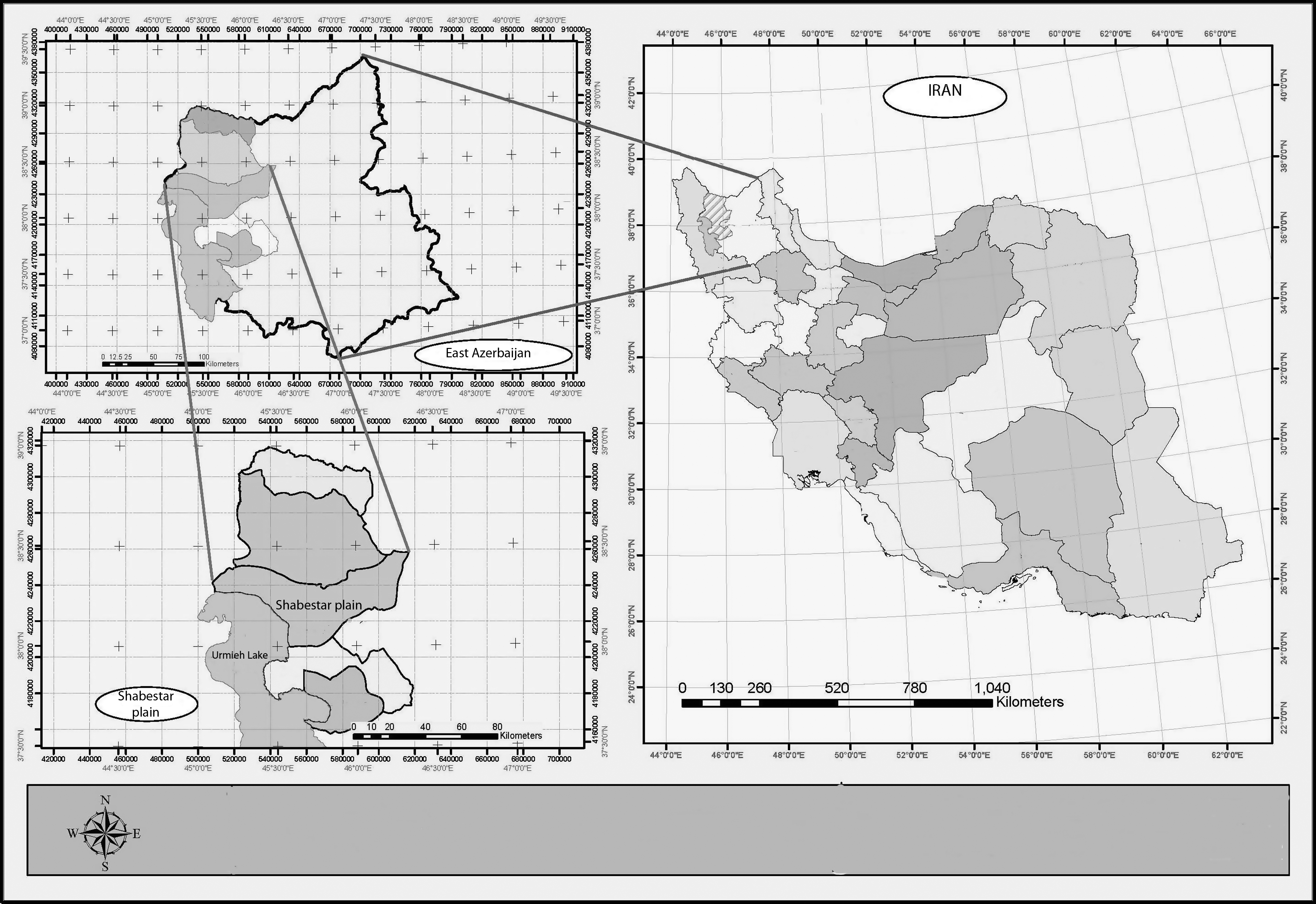
Study area.

The main daily temperature varies from −19°C in January up to 42°C in July, with a yearly average of 11°C; and the average annual rainfall is about 250 mm.

Urmieh Lake, located in northwestern Iran, is an oligotrophic lake of thalassohaline origin, the20th largest, and the second hyper saline lake in the world, with a total surface area between 4750 and 6100 km² and a maximum depth of 16 m at an altitude of 1250 m. The lake is divided into north and south parts separated by a causeway, in which a 1500 m gap provides little exchange of water between the two parts. Due to drought and increased demands for agricultural water in the lake's basin, the salinity of the lake has risen to more than 300g/L during recent years, and large areas of the lake bed have been desiccated. The possible causes of rising salinity are likely to be surface flow diversions, groundwater extractions, and unsuitable climate condition.

Fluctuation of Urmieh Lake water levels has tremendous environmental impacts, especially on the adjoining groundwater resources. About 4.4 million people live in the Urmieh Lake basin, whose irrigation economy is strongly dependent on existing surface and groundwater resources in the area. Accordingly, human population growth in the lake's basin has seriously increased the need for agricultural and potable water in recent years, all of which are supplied from surface and groundwater sources in the area. These issues, together with poor weather conditions, have significantly reduced the volume of water entering the lake so that, at present, Urmieh Lake has shrunk significantly and large areas of the former lake bed have been exposed. According to the interaction between the water depth of the lake and groundwater level of the plain, decreasing of the water depth of the lake leads to decrease of groundwater level of the plain and also increase of the groundwater salinity.

In this article, an attempt has been made at utilizing the ANN and geostatistics concepts in order to investigate the effects of the lake's water depth and other hydro-meteorological parameters on the groundwater level via spatiotemporal modeling.

The data utilized in this study were collected over 13 years (from April 1994 to March 2006) with a one-month time interval. Table 1 shows the statistical analysis of the observed groundwater levels of piezometers.

Table 1.

Statistical Analysis of Observed Data in Piezometers

	UTM
Piezometer	x (m)	y (m)	Piezometer elevations (m)	Mean (m)	Minimum (m)	Maximum (m)	Variance (m²)	Standard deviation (m)	Skewness coefficient
P1	586050	4238025	1401.48	1390.0	1389.6	1391.1	0.069140	0.262944	1.224652
P2	562800	4230450	1583.24	1547.8	1540.9	1553.8	8.785094	2.963966	−0.12895
P3	561450	4217350	1277.70	1333.7	1331.4	1336.8	1.211814	1.100824	0.132759
P4	562250	4221350	1322.79	1272.0	1268.1	1276.2	3.930377	1.982518	0.026029
P5	576925	4223350	1309.97	1297.7	1295.4	1303.4	3.523323	1.877052	1.473395
P6	577600	4222950	1303.96	1302.5	1301.7	1303.6	0.235159	0.484932	0.611962
P7	584800	4229250	1325.98	1299.1	1298.1	1301.3	0.399340	0.631933	1.321099
P8	546600	4223900	1301.86	1321.8	1319.5	1323.7	1.302649	1.141337	−0.374780
P9	551700	4220350	1292.05	1282.2	1279.0	1284.4	3.338116	1.827051	−0.346380
P10	554550	4220050	1289.02	1284.2	1282.4	1285.8	0.970875	0.985330	0.031911
P11	555050	4220250	1288.98	1285.9	1283.6	1287.3	0.805980	0.897764	−0.651490

UTM, Universal Transverse Mercator.

The monthly data collected consist of the following categories:

Observed water levels of piezometers located within the Shabestar plain (P1, P2, P3, … , P11 for training and TP1, TP2, and TP3 for cross-validation purposes). Figure 2 shows positions of the piezometers in the study area.

Rainfall in Sharafkhaneh station.

Average discharge of Daryanchai in Daryan station.

Urmieh Lake level,

Temperature in Sharafkhaneh station.

FIG. 2.

Piezometer positions.

Artificial Neural Network

ANNs offer an effective approach for handling large amounts of dynamic, nonlinear, and noisy data, especially when the underlying physical relationships are not fully understood. This makes them well suited to time-series modeling problems of a data-driven nature. In general, the advantages of an ANNs over other statistical and conceptual models can be classified as the following (Nourani et al., 2008):

The application of ANN does not require prior knowledge of the process, because ANNs have black-box properties,

1) ANNs have the inherent property of nonlinearity, as neurons activate a nonlinear filter called an activation function.

2) ANNs can have multiple inputs having different characteristics, which can represent the time-space variability.

3) ANN has been proved to be effective in modeling virtually any nonlinear function to an arbitrary degree of accuracy. The main advantage of this approach over traditional methods is that it does not require the complex nature of the underlying process under consideration to be explicit.

ANN is composed of a number of interconnected simple processing elements called neurons or nodes with the attractive attribute of information processing characteristics such as nonlinearity, parallelism, noise tolerance, learning, and generalization capability. Among the applied neural networks, the feed-forward neural networks (FFNN) with back-propagation (BP) algorithm are the most common used methods in solving various engineering problems (Nourani and Kalantari, 2010).

FFNN technique consists of layers of parallel processing elements called neurons, with each layer being fully connected to the preceding layer by interconnection strengths, or weights. Initial estimated weight values are progressively corrected during a training process that compares predicted outputs with known outputs. Learning of these ANNs is generally accomplished by BP algorithm (Hornik et al., 1989). The objective of the BP algorithm is to find the optimal weights, which would generate an output vector, as close as possible to the target values of the output vector, with the selected accuracy.

The network is determined by architecture of the network, the magnitude of the weights, and the processing element's mode of operation. The neuron is a processing element that takes a number of inputs, weights them, sums them up, adds a bias, and uses the results as the argument for a singular valued function called the transfer function. The transfer function results in the neuron's output. At the start of training, the output of each node tends to be small. Consequently, the derivatives of the transfer function and changes in the connection weights are large with regard to the input. As learning progresses and the network reaches a local minimum in error surface, the node outputs approach stable values. Consequently, the derivatives of the transfer function with regard to input, as well as changes in the connection weights, are small.

The BP neural network is the most widely used ANN in hydrologic modeling and is also used in this study. A typical BP neural network model is a full-connected neural network including input layer, hidden layer, and output layer. Various steps of the BP training procedure are described in Fig. 3.

FIG. 3.

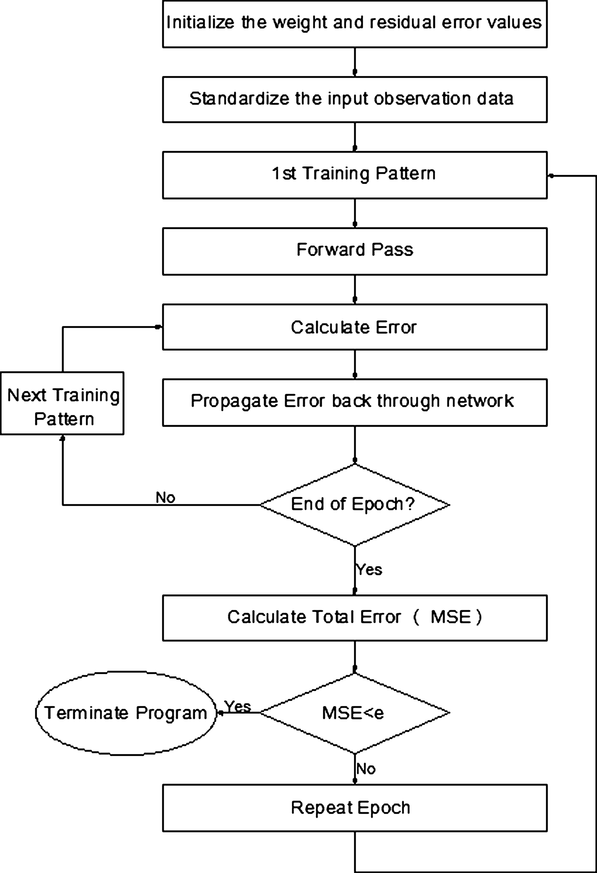
Flowchart of back-propagation algorithm.

BP algorithms use input vectors and corresponding target vectors to train ANN. The standard BP algorithm is a gradient descent algorithm, in which the network weights are changed along the negative of the gradient of the performance function. There are a number of variations in the basic BP algorithm that is based on other optimization techniques such as conjugate gradient and Newton methods (Hornik et al., 1989).

For properly trained BP networks, a new input leads to an output similar to the correct output. This ANN property enables training of a network on a representatives set of input/target pairs and achieves sound forecasting results. A clear, systematic document about the BP algorithm and the methods for designing the BP model are given by Basheer and Hajmeer (2000) and Jiang et al. (2008). Some researchers claim that networks with a single hidden layer can approximate any continuous function to a desired accuracy and are enough for most forecasting problems (Hornik et al., 1989).

In this study, at first step by using a three-layer neural network via a sensitivity analysis, the effective data sets are chosen. All input values are standardized to a specific range separately after data division. Input and output variables are preprocessed by scaling them between zero and one to eliminate their dimensions and to ensure that all variables receive equal attention during training of the models. Finally, the training and testing data sets are selected, and the network is trained.

The Levenberg-Marquardt (LM) method is a modification of the classic Newton algorithm for finding an optimum solution to a minimization problem. LM has large computational and memory requirement and, thus, it can only be used in small networks (Maier and Dandy, 1998). It is faster and less easily trapped in local minima than other optimization algorithms (Toth et al., 2000; Coulibaly et al., 2001a, 2001b, 2001c).

In this article, among the many training methods, the LM training algorithm was selected, considering its fast convergence ability (Sahoo et al., 2005). Also, a Tangent Sigmoid transfer function was used for hidden layer and a linear transfer function for the output layer according to Qu et al. (2004). The numbers of hidden layer nodes and training epochs are determined using trial and error in the test scenarios.

Geostatistics

Since detailed information about geostatistics and geostatistical techniques such as Kriging can be found in the scientific literature (e.g., Isaaks and Srivastava, 1989), only a brief description of the Kriging method, which is employed in this research, is provided.

Kriging technique is a spatial interpolation estimator Z(x₀) used to find the best linear unbiased estimator of a second-order stationary random field with an unknown constant mean:

Where Z(x₀) is Kriging estimate at location x₀; Z(x_i) is sampled value at x_i; λ_i is weighting factor for Z(x_i); and i = 1, … , n in which n denotes to the numbers of samples. The estimation error can be written as

Where Z(x₀) is unknown true value at x₀; and R(x₀) is estimation error. For an unbiased estimator, the mean of the estimates must be equal to the true mean, therefore (Ma et al., 1999):

Where E is expected value and then:

The best linear unbiased estimator must have minimum variance of estimation error. The minimization of the estimation error variance under the constraint of unbiasedness leads to a set of simultaneous linear algebraic equations for the weighting factors as follows (Ma et al., 1999):

Where Var is the abbreviation of variance function. The weighting factors λ_i can be determined by solving a nonlinear optimization problem involving the minimization of the foregoing function subject to the constraint in (4) by using the Lagrange multiplier μ as

The necessary conditions for optimal λ_i and μ values involve setting the first derivative of equation (6) to zero; therefore, the system of simultaneous linear algebraic equations for λ_i and μ can be expressed in matrix form as (Ma et al., 1999):

\documentclass{aastex}\usepackage{amsbsy}\usepackage{amsfonts}\usepackage{amssymb}\usepackage{bm}\usepackage{mathrsfs}\usepackage{pifont}\usepackage{stmaryrd}\usepackage{textcomp}\usepackage{portland,xspace}\usepackage{amsmath,amsxtra}\pagestyle{empty}\DeclareMathSizes{10}{9}{7}{6} \begin{document} \begin{align*} \left[\begin{matrix} \gamma_{11} & \gamma_{12} & \cdots & \gamma_{1n} & 1 \\ \gamma_{21} & \gamma_{22} & & \gamma_{2n} & 1 \\ \vdots & & \ddots & \vdots & \\ \gamma_{n1} & \gamma_{n2} & \cdots & \gamma_{nn} & 1 \\ 1 & 1 & \ldots & 1 & 0\end{matrix} \right] \left[ \begin{matrix} \lambda_1 \\ \lambda_2 \\ \vdots \\ \lambda_n \\ \mu\end{matrix} \right] = \left[ \begin{matrix} \gamma_{01} \\ \gamma_{02} \\ \vdots \\ \gamma_{0n} \\ 1\end{matrix} \right] \tag{7} \end{align*} \end{document}

The Variogram γ can be derived from sampled data as follows:

The presence of a spatial structure where observations close to each other are more alike than those that are far apart (spatial autocorrelation) is a prerequisite to the application of geostatistics. The experimental Variogram measures the average degree of dissimilarity between un-sampled values and a nearby data value and, thus, can depict autocorrelation at various distances. The value of the experimental Variogram for a separation distance of h (referred to as the lag) is half the average squared difference between the value at Z(x_i) and the value at Z(x_i+h) as (Ma et al., 1999):

Where n is the number of data pairs within a given class of distance and direction. If the values of Z(x_i) and Z(x_i+h) are auto correlated, the results of equation (8) will be small, relative to an uncorrelated pair of points. From analysis of the experimented Variogram, a suitable model (e.g., spherical, exponential) is then fitted, usually by weighted least squares; and the parameters (e.g., range, nugget and sill) are then used in the Kriging procedure (Isaaks and Srivastava, 1989).

Proposed Hybrid Model and Results

By combining the ANN capability in modeling complicated and nonlinear systems and geostatistical ability in linear estimation with low estimation error, a hybrid model of spatiotemporal groundwater level forecasting in a coastal aquifer has been proposed in this article that uses both the mentioned models in a unique framework. Figure 4 shows the proposed model scheme.

FIG. 4.

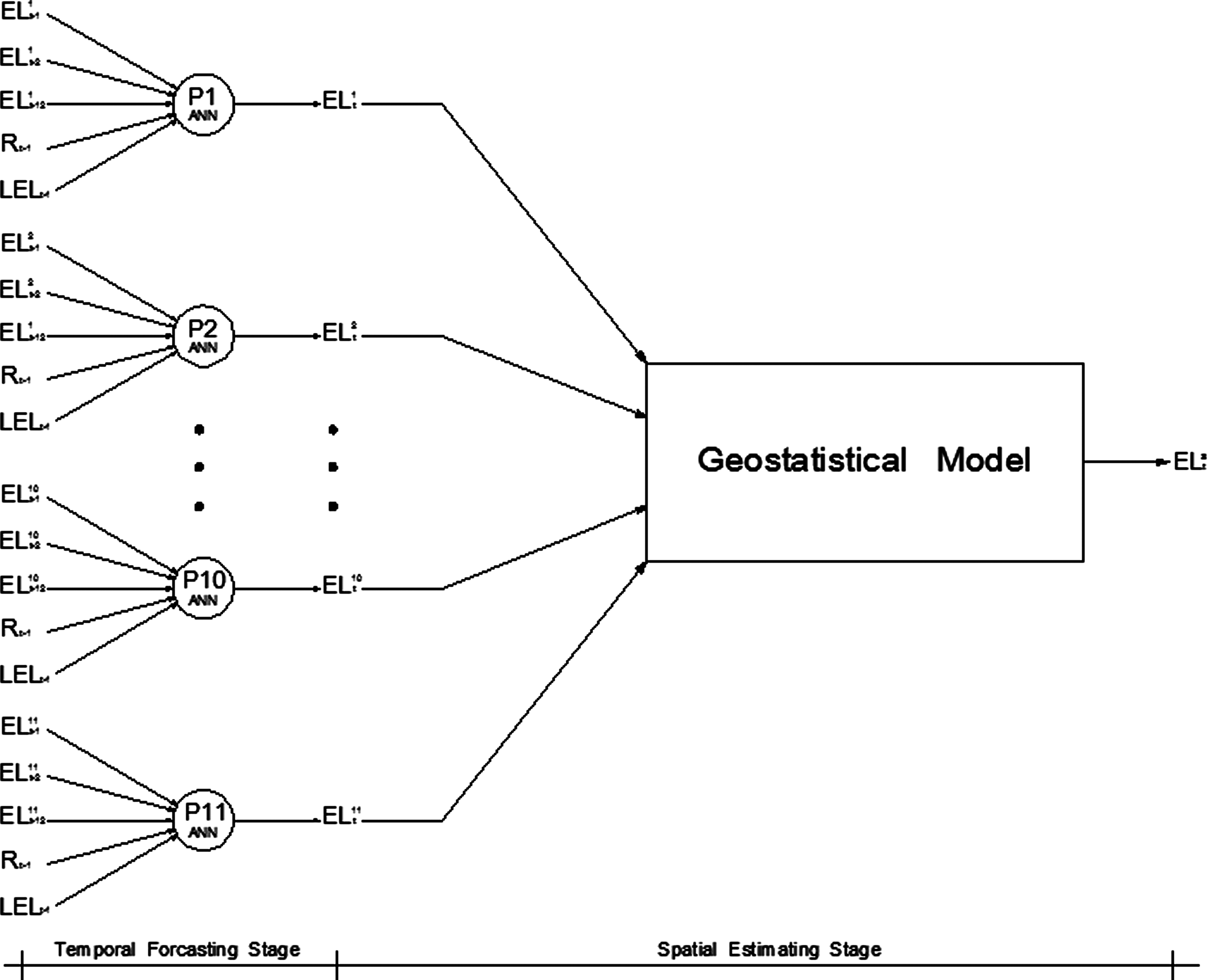
Diagram of proposed hybrid model.

The proposed model contains two separated stages. At the first stage, an ANN is trained for each piezometer (P1, P2, … , P11) for time series modeling of the water level. The model predicts the next month's groundwater level of the piezometer based on quantity of present month rainfall in study area (R_t-1), Urmieh Lake water surface level at that month (LEL_t-1), and groundwater levels in present, first, and twelfth previous months (EL_t-1,EL_t-2,EL_t-12) in order to handle the seasonality of the process as well as the autoregressive characteristics. A sensitivity analysis was employed to select the mentioned input parameters from all the available data, as will be discussed in the next section.

At the second stage, the predicted values of water levels at different piezometers are imposed to a calibrated geostatistics model in order to estimate groundwater level at any desired point in the plain. Finally, as a cross-validation process, the proposed spatiotemporal model is evaluated by the data of piezometers TP1,TP2, and TP3, which do not contribute in the calibration step of the model. The details and results of the stages are presented in the following sections.

Temporal forecasting stage

In order to ensure good generalization ability by an ANN model, some empirical relationships between the number of training samples and the number of connection weights have been suggested in the literature. However, network geometry is generally highly problem dependent, and these guidelines do not ensure optimal network geometry, where optimality is defined as the smallest network that adequately captures the relationships in the training data (principle of parsimony). In addition, there is quite a high variability in the number of input and hidden nodes suggested by the various rules. Although research is being conducted in this direction by the scientists working in ANNs, it may be noted that traditionally, optimal network geometries have been found by trial and error (Maier and Dandy, 2000). Consequently, in the current application, the number of hidden neurons in the network, which is responsible for capturing the dynamic and complex relationship between various input and output variables, was identified by several trials. Also, this trial-and-error procedure with domain knowledge was explored for general guidance in the number of inputs selected.

The trial-and-error procedure initially started with two hidden neurons, and the number of hidden neurons was increased up to fifty with a step size of one in each trial. For each set of input and hidden neurons, the network was trained in batch mode to minimize the mean square error at the output layer. In order to check any over-fitting during training, a validation was performed by keeping track of the efficiency of the fitted model. The training was stopped when there was no significant improvement in the efficiency. The parsimonious structure that resulted in minimum root mean squared error (RMSE) (equation 9) and maximum efficiency coefficient (equation 10) during training as well as testing was selected as the final form of the ANN model for each piezometer.

The variables are scaled to a limit between zero and one as the activation function warrants. The total available data were divided into two sets, calibration and validation sets. In the training step, the models were trained using data of ten years (1994–2003) and then validated on the rest of the data (2004–2006).

The RMSE and coefficient of efficiency (CE) were used to assess the effectiveness of each model and its ability to make precise predictions. The RMSE is calculated by

Where y_i and \documentclass{aastex}\usepackage{amsbsy}\usepackage{amsfonts}\usepackage{amssymb}\usepackage{bm}\usepackage{mathrsfs}\usepackage{pifont}\usepackage{stmaryrd}\usepackage{textcomp}\usepackage{portland,xspace}\usepackage{amsmath,amsxtra}\pagestyle{empty}\DeclareMathSizes{10}{9}{7}{6} \begin{document} $${\hat y}_i$$ \end{document} are the observed and predicted data, respectively, and N is the number of observations. RMSE indicates the discrepancy between the observed and calculated values. The lowest the RMSE, the more accurate the prediction is. Nash and Sutcliffe (1970) proposed the nondimensional CE criterion on the basis of standardization of the residual variance with initial variance, which provides a measure for the proportion of the variance explained by the model. It can be used to compare the relative performances of the models that are developed by different methods. It is estimated as (Nash and Sutcliffe, 1970).

Where \documentclass{aastex}\usepackage{amsbsy}\usepackage{amsfonts}\usepackage{amssymb}\usepackage{bm}\usepackage{mathrsfs}\usepackage{pifont}\usepackage{stmaryrd}\usepackage{textcomp}\usepackage{portland,xspace}\usepackage{amsmath,amsxtra}\pagestyle{empty}\DeclareMathSizes{10}{9}{7}{6} \begin{document} $${\overline y}_i$$ \end{document} is the average of observed values and the CE represents the initial uncertainty explained by the model. The CE varies between −∞, 1; and the best fit between observed and calculated values would have CE = 1. The quality of the fit statistics is measured by RMSE and CE between the computed and observed data. The sensitivity analysis to select the input neurons of the ANNs showed that present-month rainfall, lake water surface level at that month, and groundwater levels in first, second, and twelfth previous months are the most dominant parameters in forecasting the groundwater level in the most of piezometers; and these parameters were considered as the input neurons for all ANNs. For instance, the result of the sensitivity analysis for P8 has been presented in Table 2, which shows that temperature and water discharge can be ignored in the modeling. The results of temporal modeling of groundwater levels in piezometers P1, P2, … , P11, as the first stage of the hybrid modeling have been briefly shown in Table 3.

Table 2.

Sensitivity Analysis Results for Piezometer No. 8

Calibration CE	Calibration RMSE (m)	Validation CE	Validation RMSE (m)	Groundwater Level in t-1	Groundwater Level in t-2	Groundwater Level in t-12	Discharge	Rainfall	Temperature	Lake Level
0.88	0.12	0.79	0.17	√	√	√	√	-	-	-
0.91	0.08	0.81	0.16	√	√	√	√	-	-	√
0.82	0.16	0.76	0.2	√	√	√	√	-	√	-
0.81	0.17	0.80	0.16	√	√	√	√	-	√	√
0.83	0.15	0.77	0.19	√	√	√	-	-	√	-
0.84	0.14	0.78	0.18	√	√	√	-	-	√	√
0.89	0.10	0.81	0.15	√	√	√	-	-	-	√
0.89	0.09	0.82	0.14	√	√	√	-	√	-	-
0.86	0.12	0.78	0.17	√	√	√	√	√	-	-
0.84	0.14	0.77	0.19	√	√	√	√	√	√	-
0.87	0.12	0.79	0.16	√	√	√	√	√	√	√
0.91	0.07	0.82	0.13	√	√	√	√	√	-	√
0.84	0.14	0.78	0.18	√	√	√	-	√	√	-
0.86	0.13	0.79	0.16	√	√	√	-	√	√	√
0.90	0.08	0.82	0.12	√	√	-	-	√	-	√
0.94	0.03	0.86	0.08	√	√	√	-	√	-	√

CE, coefficient of efficiency; RMSE, root mean squared error.

Table 3.

Artificial Neural Network Results for Temporal Forecasting Stage

	UTM				Calibration		Validation
Piezometer	x	y	Structure	Epoch No.	CE	RMSE (m)	CE	RMSE (m)
P1	586050	4238025	(5,11,1)	40	0.82	0.1	0.72	0.15
P2	562800	4230450	(5, 8,1)	100	0.93	0.09	0.86	0.12
P3	561450	4217350	(5,8,1)	100	0.92	0.07	0.85	0.1
P4	562250	4221350	(5,8,1)	100	0.92	0.08	0.83	0.12
P5	576925	4223350	(5,9,1)	80	0.86	0.07	0.78	0.13
P6	577600	4222950	(5, 9,1)	80	0.88	0.06	0.8	0.11
P7	584800	4229250	(5,10,1)	60	0.84	0.09	0.75	0.12
P8	546600	4223900	(5,6,1)	140	0.94	0.03	0.86	0.05
P9	551700	4220350	(5,6,1)	140	0.93	0.04	0.87	0.6
P10	554550	4220050	(5,7,1)	120	0.92	0.05	0.88	0.07
P11	555050	4220250	(5,7,1)	120	0.94	0.04	0.86	0.08

Spatial estimation stage

Kriging is a geostatistical technique for estimating attribute values at a point, over an area, or within a volume. It is often used to interpolate grid node value in mapping and contouring application. In theory, no other interpolation process can produce better estimates (being unbiased, with minimum error), though the effectiveness of the technique actually depends on accurately modeling the Variogram.

The accuracy of Kriging estimate is driven by the use of Variogram models to express autocorrelation relationship between control points in the data set. Kriging also produces a variance estimate for its interpolation values.

The difference between Ordinary Kriging (OK) and Universal Kriging variants residing in the model is the presence or absence of trend (Goovaerts, 1999). The main reason for using the OK model instead of Universal Kriging in the current research is the possibility of removing the bedrock elevation trend in spatial stage of modeling. Similar methodology was also conducted and reported by Yang et al. (2007); Ma et al. (1999); Cay and Uyan (2009). Also, as mentioned by Ta'any et al. (2009), this type of Kriging (i.e., Ordinary) can be used in the presence or absence of spatial trend after some modifications.

The Variogram measures dissimilarity, or increasing variance between points (decreasing correlation), as a function of distance. In addition to helping us assess how values at different location vary over distance, the Variogram provide a way to study the influence of other factors that may affect whether the spatial correlation varies only with distance (the isotropic case) or with direction and distance (the anisotropic case).Variogram map provides a visual picture of semivariance in every compass direction. If there is anisotropy, this allows one to easily find the appropriate principal axis for defining the anisotropic Variogram model. In this map, the surface (z-axis) is semivariance, and the x and y axes are separation distances in E-W and N-S directions, respectively. The center of the map corresponds to the origin of the Variogram γ(h) = 0 for every direction.

At stage two of the current modeling, which deals with spatial prediction of groundwater level, estimated groundwater level of the next month at the location of each piezometer was first corrected via bedrock elevation at the same location due to termination of existing trends (see Fig. 5). Afterward, the Variogram map of the study area was plotted using the temporally averaged values of the groundwater levels at different piezometers.

FIG. 5.

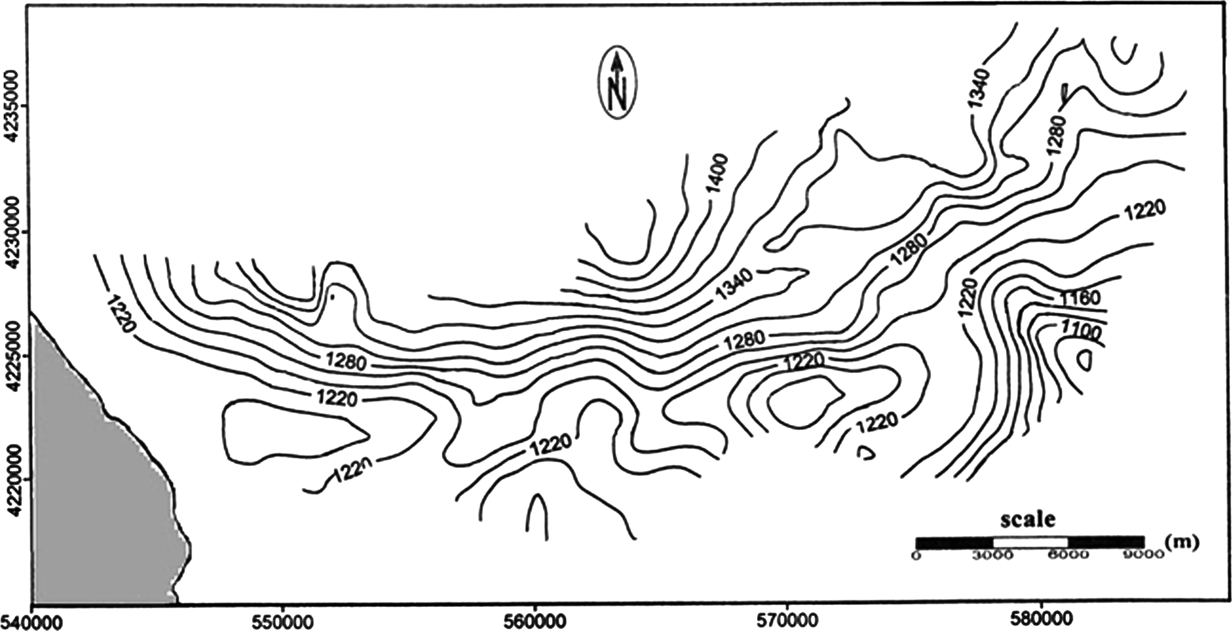
Bedrock elevations in study area (units in meters).

Figure 6 shows that the isotropic spatial modeling of the groundwater levels could be taken in use.

FIG. 6.

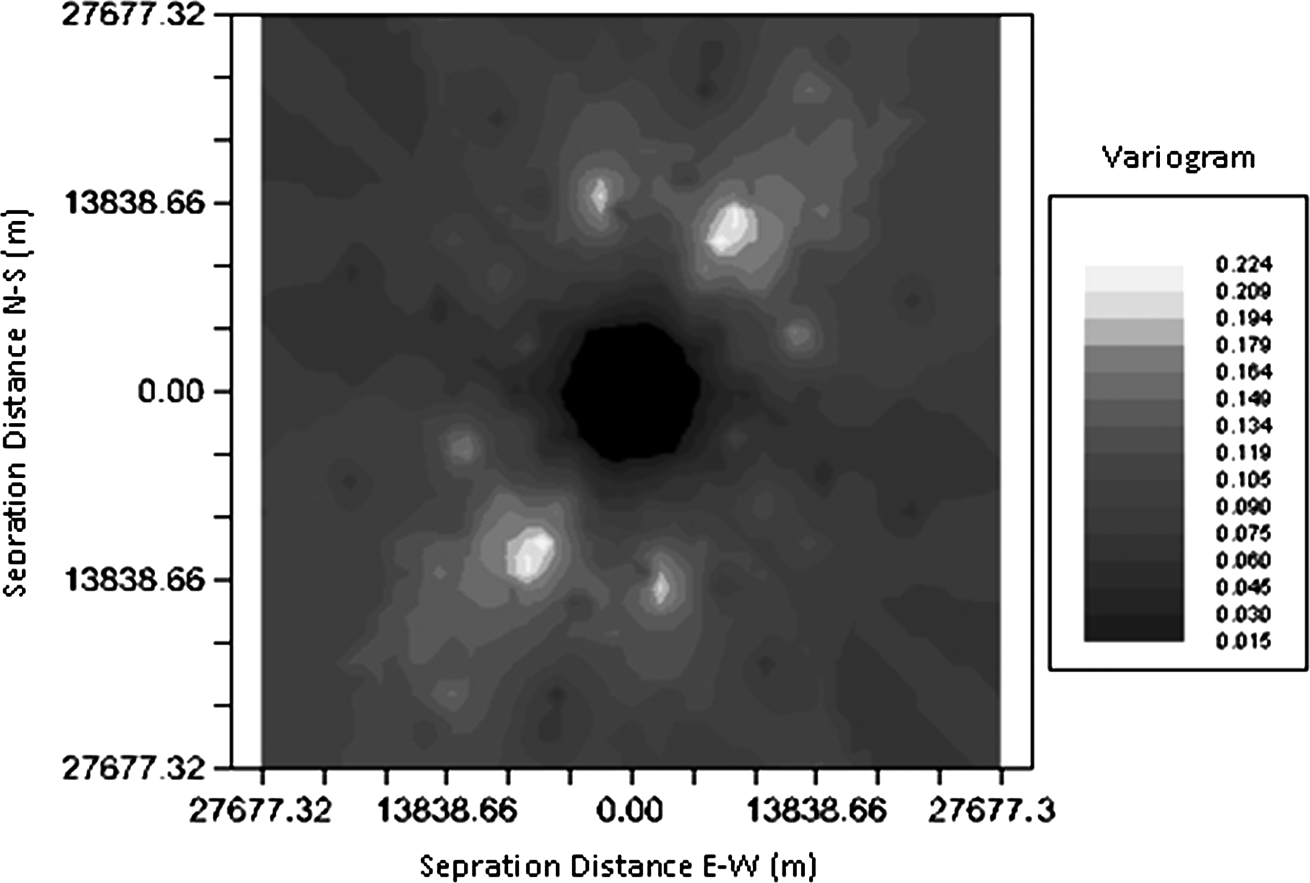
Variogram map (units in meters).

Thereafter, a suitable Variogram model was determined by fitting some well-known Variogram models (i.e., spherical, exponential, and Gaussian) to the experimental Variogram by using weighted least-squares method (Myers, 1982).

The geostatistical model, which leads to the least RMSE, was selected by comparing the observed water-table values with the values estimated by Variogram models.

According to Table 4 the best-fitted model was Gaussian model, and its parameters (i.e., range, nugget, and sill) were then used in the Kriging procedure.

Table 4.

Cross-Validation Results of Different Variogram Models

Variogram model	RMSE (m)
Exponential	3.24
Gaussian	0.35
Spherical	1.86

The selected Gaussian model is shown in Fig. 7, which is similar to the exponential model but assuming a gradual rise for the y-intercept. This model is described by the following formula (Goovaerts, 1997):

FIG. 7.

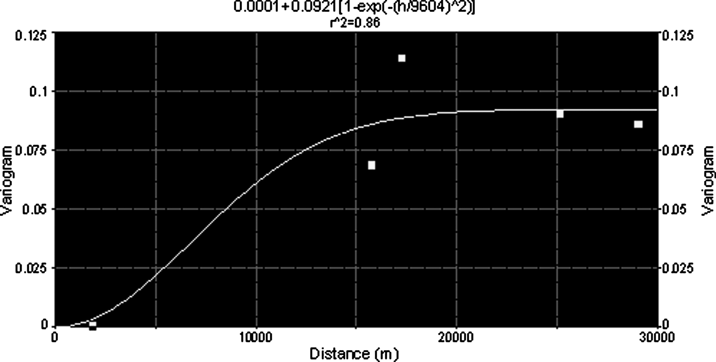
Selected variogram model.

Where: h = lag interval,

C₀ = nugget variance ≥0,

C = structural variance ≥C₀, and

A₀ = range parameter.

The range parameter in this model is simply a constant defined as that point at which 95% of the sill is approached. The range can be estimated as 1.73A₀ (1.73 is the square root of 3).

Based on the mentioned Variogram model, spatial groundwater-level estimation of the area has been carried out using Kriging method. The calibrated Kriging method was then verified via a cross-validation technique. Cross validation is a process for checking the compatibility between a set of data, the spatial model, and neighborhood design. In cross validation, each point in the spatial model is individually removed from the model, and then its value is estimated by a covariance model. In this way, it is possible to complete estimated versus actual values. Figure 8 shows the results of cross-validation procedure as a scatter plot, which denotes the reliability of the proposed geostatistical modeling.

FIG. 8.

Cross-validation results.

At this moment, both stages of the hybrid model have been completed, and the model can be used for spatiotemporal modeling of groundwater level within the Shabestar plain.

Finally, the proposed hybrid model was validated using the verification data set (2004–2006, 3 years) of piezometers TP1, TP2, and TP3, which have been utilized neither for training the ANNs nor for the calibration of the geostatistics model. For this purpose, the forecasted values of the water-level time series at different piezometers (P1, P2, … , and P11) via the trained ANNs models for the verification data set (2003 to 2006) were imposed to the calibrated geostatistical model in order to estimate the water level of piezometers TP1,TP2, and TP3, time step by time step.

The results of the modeling have been presented in Fig. 9, which demonstrates the capability of the proposed time-space hybrid model.

FIG. 9.

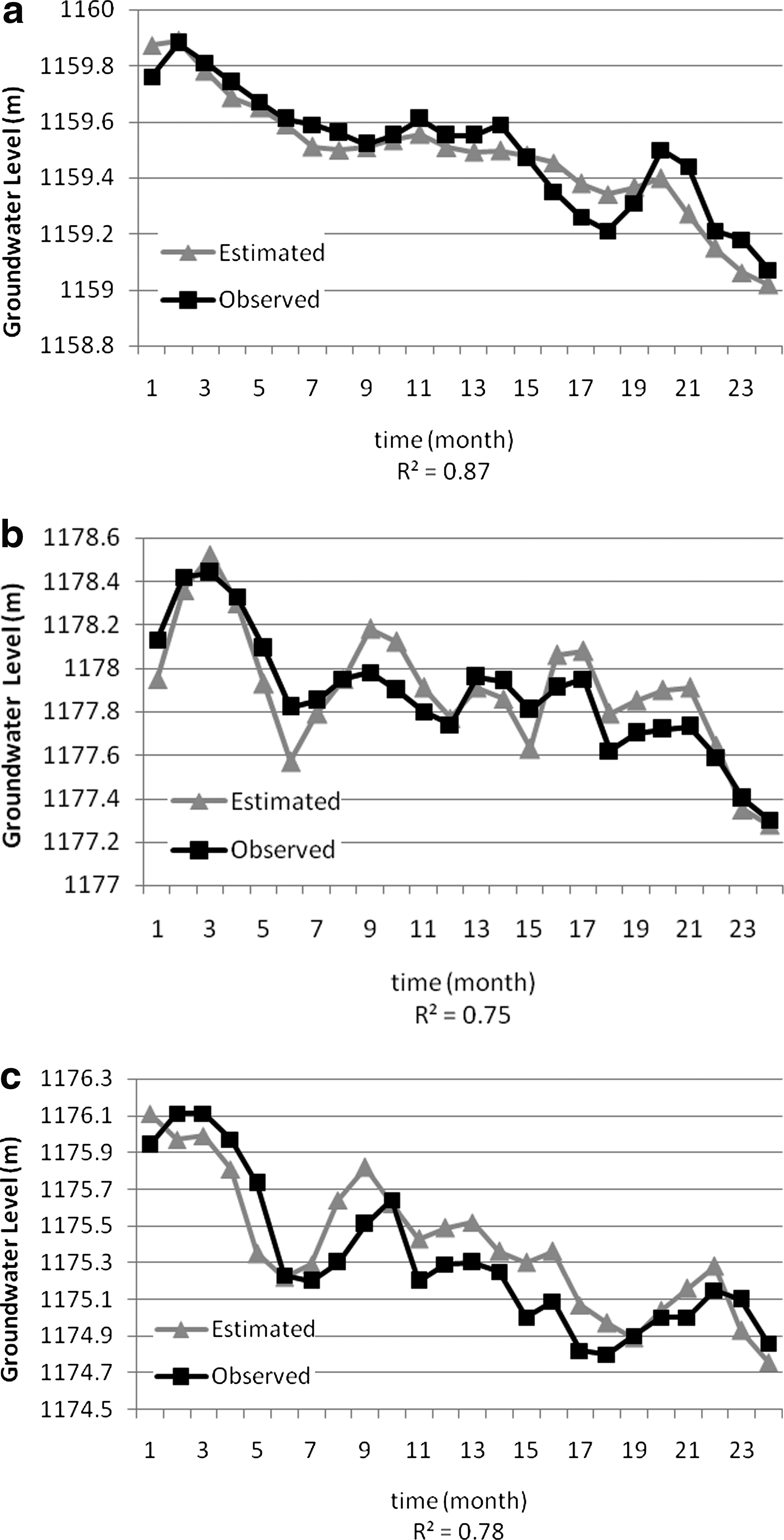
Results of spatiotemporal modeling for piezometers; (a) TP1, (b) TP2, and (c) TP3.

According to the obtained results, it can be clearly seen that the model is more capable to estimate the groundwater levels that are close to the lake. Since the water depth of lake is considered as an input variable to the ANNs, the proposed model could simulate the groundwater level of the near region to the lake more accurate than the far points.

Concluding Remarks

There are many hydrological variables that can be viewed as spatiotemporal phenomena. For example, monthly rainfalls or piezometric readings exhibit random aspects both with regard to time and space. The estimation of such variables at unsampled spatial locations or unsampled times requires the adequate thechniques into space-time domain. In this study, according to inherent capability of ANNs in temporal forecasting and geostatistics in spatial estimating, the potential of the proposed hybrid empirical model (ANNG) was evaluated for the purpose of spatiotemporal prediction of groundwater levels in a coastal aquifer in Iran.

Monthly groundwater levels data from eleven piezometers (P1, P2, … P11), rainfall, and lake-water surface elevations in the 13 years are the inputs of multilayer FFNN. Kriging was applied to the outputs from ANN models to estimate groundwater levels in unsampled locations such as coordinates of three selected piezometers (TP1, TP2, and TP3).

This modeling framework is applied for the Shabestar plain, which is located in northwest Iran at Azerbaijan province. The major results of the study are summarized as follows:

The results of the research reported in the article show high efficiency of three-layer BPANN with LM training algorithm for groundwater elevation prediction in the case study for a coastal aquifer.

Due to spatial structure between groundwater levels in adjacent points of the coastal aquifer, application of Kriging with isotrope Gaussian Variogram geostatistical model led to appropriate results.

In general, the results of the case study are satisfactory and demonstrate that the proposed hybrid model (ANNG) is a promising spatiotemporal prediction tool for groundwater modeling and may be also employed to fill the temporally and/or spatially missed data.

In order to complete the current study, it is suggested to extend the presented model for estimation of some qualitative parameters of the groundwater such as salinity via a multivariate geostatistics tool (e.g., Cokriging). Further, the application of wavelet transform or adding some forecasting sub-models for modeling the input hydrologic parameters of the model (e.g., precipitation, lake's water depth … ) (Nourani et al., 2009b) and/or clustering approach, respectively, as spatio temporal data preprocessing techniques, may improve the efficiency of the proposed model.

Footnotes

Author Disclosure Statement

No competing financial interests exist.

References

Aboufirassi

, Marino

M.A.

1983. Kriging of water level in the Souss aquifer, Morocco. Math. Geol., 15:537.

Alvisi

, Mascellani

, Franchini

, Bardossy

2006. Water level forecasting through fuzzy logic and artificial neural network approach. Hydrol. Earth Sys. Sci., 10:1.

ASCE Task Committee. 1990a. Review of geostatistics in geohydrology, part I: basic concepts. J. Hydraulic Eng., 116:612.

ASCE Task Committee. 1990b. Review of geostatstics in geohydrology, part II: applications. J. Hydraulic Eng., 116:633.

ASCE Task Committee. 2000a. Artificial neural networks in hydrology, part I: preliminary concepts. J. Hydrol. Eng., 5:115.

ASCE Task Committee. 2000b. Artificial neural networks in hydrology, part II: hydrologic application. J. Hydrol. Eng., 5:124.

Barca

, Passarella

2008. Spatial evaluation of the risk of groundwater quality degradation. A comparsion between disjunctive Kriging and geostatistical simulation. Environ. Monit. Assess., 137:261.

Basheer

I.A.

, Hajmeer

2000. Artificial neural networks: fundamentals, computing, design, and application. J. Microbiol. Methods, 43:3.

Beaudeau

, Leboulanger

, Lacroix

, Hanneton

, Wang

H.Q.

2001. Forecasting of turbid floods in a karstic drain using an artificial neural network. Ground Water, 39:139.

10.

Cay

, Uyan

2009. Spatial and temporal groundwater level variation geostatistical modeling in the city of Konya, Turkey. Water Environ. Res., 12:2460.

11.

Coppola

, Poulton

, Charles

, Dustman

, Szidarovszky

2003. Application of artificial neural networks to complex groundwater management problems. Nat. Resour. Res., 12:303.

12.

Coppola

, Rana

A.J.

, Poulton

, Szidarovszky

, Uhi

V.W.

2005. A neural networks model for prediction aquifer water level elevation. Ground Water, 43:231.

13.

Coulibaly

, Anctil

, Aravena

, Bobee

2001a. Artificial neural network modeling of water table depth fluctuation. Water Resour. Res., 37:885.

14.

Coulibaly

, Anctil

, Bobee

2001b. Multivariate reservoir inflow forecasting using temporal neural networks. J. Hydrol. Eng., 9–10:367.

15.

Coulibaly

, Bobee

, Anctil

2001c. Improving extreme hydrologic events forecasting using a new criterion for artificial neural network selection. Hydrol. Process., 15:1533.

16.

Daliakopoulos

, Coulibaly

, Tsanis

I.K.

2005. Groundwater level forecasting using artificial neural networks. J. Hydrol., 309:229.

17.

Delhomme

J.P.

1978. Kriging in hydrosciences. Adv. Water Resour., 1:251.

18.

Dogan

, Demirpence

, Cobaner

2008. Prediction of groundwater levels from lake levels and climate data using ANN approach. Water SA, 34:199.

19.

Finke

P.A.

, Brus

D.J.

, Bierkens

M.F.P.

, Hoogland

, Knotters

, Vries

2004. Mapping groundwater dynamics using multiple sources of exhaustive high resolution data. Geoderma, 123:23.

20.

Goovaerts

1997. Geostatistics for Natural Resources Evaluation. New York: Oxford University Press.

21.

Goovaerts

1999. Geostatistics in soil science: state-of-the-art and perspectives. Geoderma., 89:1.

22.

Govindaraju

R.S.

, Ramachandra

R.A.

2000. Artificial Neural Networks in Hydrology. Netherlands: Kluwer Academic Publishing.

23.

Hopfield

J.J.

1982. Neural networks and physical systems with emergent collective computational abilities. Proc. Natl. Acad. Sci. USA, 79:2554.

24.

Hornik

, Stinchcombe

, White

1989. Multilayer feed forward networks are universal approximators. Neural Netw., 2:359.

25.

Isaaks

E.H.

, Srivastava

R.M.

1989. Applied Geostatistics. New York: Oxford University Press.

26.

Jiang

S.Y.

, Ren

Z.Y.

, Xue

K.M.

, Li

C.F.

2008. Application of BPANN for prediction of backward ball spinning of thin-walled tubular part with longitudinal inner ribs. J. Mater. Process. Technol., 196:190.

27.

Lallahem

, Mania

2003. Evaluation and forecasting of daily groundwater inflow in a small chalky watershed. Hydrol. Process., 17:1561.

28.

Lallahem

, Mania

, Hani

, Najjar

2005. On the use of neural networks to evaluate groundwater levels in fractured media. J. Hydrol., 307:92.

29.

T.S.

, Sophocleous

, Yu

Y.S.

1999. Geostatistical applications in groundwater modeling in south-central Kansas. J. Hydrol. Eng., 16:57.

30.

Maier

H.R.

, Dandy

G.C.

1998. Understanding the behavior and optimizing the performance of back-propagation neural network: an empirical study. Environ. Model. Softw., 13:179.

31.

Maier

H.R.

, Dandy

G.C.

2000. Neural network for the prediction and forecasting water resources variables: a review of modeling issues and applications. Environ. Model. Softw., 15:101.

32.

Matheron

1963. Principles of geostatistics. Econ. Geol., 58:1246.

33.

McCulloch

W.S.

, Pitts

1943. A logical calculus of the ideas immanent in nervous activity. Bull. Math. Biophys., 5:115.

34.

Myers

D.E.

1982. Matrix formulation of Cokriging. Math. Geol., 14:249.

35.

Nash

J.E.

, Sutcliffe

J.V.

1970. River flow forecasting through conceptual models: part I. A conceptual models discussion of principles. J. Hydrol., 10:282.

36.

Neuman

S.P.

, Jacobsen

E.A.

1984. Analysis of nonintrinsic spatial variability by residual kriging with application to regional groundwater level. Math. Geol., 16:499.

37.

Nourani

, Alami

M.T.

, Aminfar

M.H.

2009a. A combined neural-wavelete model for prediction of Ligvanchai watershed precipitation. Eng. Appl. Artif. Intell., 22:466.

38.

Nourani

, Kalantari

2010. An integrated artificial neural network for spatiotemporal modeling of rainfall-runoff-sediment processes. Environ. Eng. Sci., 27:411.

39.

Nourani

, Komasi

, Mano

2009b. A multivariate ANN-wavelet approach for rainfall-runoff modeling. Water Resour. Manag., 23:2877.

40.

Nourani

, Mano

2007. Semi-disrtibuted flood runoff model at the sub continental scale for southwestern Iran. Hydrol. Process., 21:3137.

41.

Nourani

, Mogaddam

A.A.

, Nadiri

2008. An ANN-based model for spatiotemporal groundwater level forecasting. Hydrol. Process., 22:5054.

42.

Z.Y.

, Chen

Y.X.

, Shi

H.B.

2004. Structure and algorithm of BP network for underground hydrology forecasting. J. Water Resour., 2:88.

43.

Rajaee

, Mirbagheri

S.A.

, Kermani

, Nourani

2009. Daily suspended sediment concentration simulation using ANN and neuro-fuzzy models. Sci. Total Environ., 407:4916.

44.

Rumelhart

D.E.

, McClelland

J.L.

1986. Parallel Distributed Processing: Explorations in the Microstructure of Cognition, I and Ii. Cambridge: MIT Press.

45.

Sahoo

G.B.

, Raya

, Wadeb

H.F.

2005. Pesticide prediction in groundwater in North Carolina domestic wells using artificial neural network. Ecol. Model., 183:29.

46.

Ta'any

, Tahboub

, Saffarini

2009. Geostatistical analysis of spatiotemporal variability of groundwater level fluctuations in Amman-Zarqa basin, Jordan: a case study. Environ. Geol., 57:525.

47.

Tayfur

, Singh

V.P.

2006. ANN and fuzzy logic models for simulating event-based rainfall-runoff. J. Hydraulic Eng., 132:1321.

48.

Tayfur

, Swiatek

, Wita

, Singh

V.P.

2005. Case study: finite element method and artificial neural network models for flow through Jeziorsko earth dam in Poland. J. Hydraulic Eng., 131:431.

49.

Toth

, Brath

, Montanari

2000. Comparsion of short-term rainfall prediction models for real-time flood forecasting. J. Hydrol., 239:132.

50.

Yang

, Cao

, Liu

, Yang

2007. Design of groundwater level monitoring network with Ordinary Kriging. J. Hydrodynamics, 20:339.