Development of a Complex System Dynamic Eutrophication Model: Application to Karkheh Reservoir

Abstract

The ever-increasing pollutant loads have significantly degraded the quality of receiving water bodies. High–resolution, spatially distributed water quality simulation models can be unsuitable at the planning/reconnaissance level of water resources decision making or for the rapid interactive analysis to support a participatory decision environment. This study presents a complex system dynamic (SD) eutrophication model in an object-oriented template to facilitate reservoir nutrient simulation process and assessment of alternative management strategies. The proposed model considers feedback and interactive loops between phytoplanktons, herbivorous zooplanktons, carnivorous zooplanktons, particulate organic matter, dissolved organic matter, ammonium, nitrate, phosphorus, total suspended solids, and dissolved oxygen in the simulation process. The reservoir SD eutrophication model is structured and expressed as a series of 30 differential equations for 10 state variables and three segmented layers. The model was applied to the Karkheh Reservoir in Iran to simulate the key epilimnion, thermocline, and hypolimnion temporal patterns of the system. The SD eutrophication model is quite suitable for rapid scenario analysis and preliminary management targets. Results of the proposed model compared well with those of a well-known two-dimensional process-based water quality simulation model (CE-QUAL-W2) and measured field data during the calibration and verification periods. Effects of reduction and/or increase in total incoming nutrient loads resulting from different load management scenarios were also examined. Results showed that the Karkheh Reservoir is phosphorus limited during the summer stratified periods.

Introduction

During the past few decades, population growth and the development of industries and municipalities have led to increased loading of various pollutants into water bodies. The Karkheh Reservoir, the largest man-made reservoir in Iran, has experienced an increasing trend of algae growth and water quality degradation during the last few years. Based on the available field data and evidence reported by the operators, the reservoir is considered susceptible to eutrophication, because it has been subjected to increased loading from upstream watershed. Relatively long residence time of the reservoir, increasing nutrient load, and strategic purposes of the reservoir demand detailed modeling, monitoring, and assessment of eutrophication formation.

Reservoir eutrophication systems have a high level of dynamic complexity. Studies about the causes and consequences of eutrophication and potential mitigating actions are complex for any lake or impoundment (Tufford and McKellar, 1999). Existence of a number of “causes and consequences feedback loops” with the dynamically varying eutrophication process imposes a dynamic complexity to the problem.

Combination of mathematical models and monitoring provide powerful tools to assess the effects of management decisions prior to their implementation and also to represent reservoir water quality (WOTSP, 2004). Water quality models are of different types intended to serve different purposes. The steady-state, input-output equations of Vollenweider (1975) and Dillon and Rigler (1974) have been extensively used as classical modeling approaches to address lake eutrophication. These models are not capable of predicting the dynamic trend of eutrophication in a large reservoir with temporal variation in inflow and storage. An alternative to these “data-oriented” models is “process-oriented” water quality models, which have a more explicit mechanistic basis and include chemical/biological interactions usually not taken into account in mass balance models (Arhonditsis et al., 2002). The process-oriented models are usually data-intensive and frequently over-parameterized, and are therefore useful in a wide variety of applications related to surface water quality. During the last two decades, significant progress has been made in the development and application of process-based multidimensional hydrodynamics and water quality models (Cerco and Cole, 1993; Jin et al., 1998; Gin et al., 2001; Arhonditsis et al., 2002; Kuo et al., 2003; Wu et al., 2004; Kuo et al., 2006; Gelda and Effler, 2007; Diogo et al., 2008; Li et al., 2008).

Although process-based high-resolution models provide detailed temporal and spatial analysis of reservoir water quality dynamics, for real-time, interactive scenario analysis, such models can be limiting for some main reasons. First, the text-based input files cannot be easily manipulated for real-time interactive scenario testing. Second, the minutes or several minutes is required for spatially complex reservoir water quality models (Roach and Tidwell, 2009).

In the system dynamic (SD) approach, the problem is characterized dynamically, that is, as a pattern of behavior, unfolding over time, which shows how the problem arose and how it might evolve in the future (Forrester, 1961; Sterman, 2000). The SD approach is used in different fields of science, such as water quantity and quality management, transportation, and land use management (Vezjak et al., 1998; Simonovic and Fahmy, 1999; Heimgartner, 2001; Ahmad and Simonovic, 2004; Viste and Skartveit, 2004; Luo et al., 2005; Elmahdi et al., 2007).

This study presents an object-oriented eutrophication model employing SD approach to facilitate addressing reservoir response to the management activities. A key purpose of the model described here is to create a rapid reservoir water quality module that considers interactions among water quality of the spatial elements (adjacent layers), changes or alterations in the structure and function over time, adaptation, and counterintuitivity. The proposed model considers feedback and interactive loops between phytoplanktons, herbivorous zooplanktons, carnivorous zooplanktons, particulate organic matter (POM), dissolved organic matter (DOM), ammonium, nitrate, phosphorus, total suspended solids (TSS), and dissolved oxygen (DO). The developed model is a semi-distributed eutrophication model, which is quite beneficial for planning purposes when only limited data are available and a rapid eutrophication assessment under different management strategies is needed. The model intends to (1) present a clear conceptual eutrophication modeling scheme in an object-oriented template, which provides an ideal environment for shared vision modeling and negotiations between the different parties involved; and (2) provide a partially simplified structure of reservoir eutrophication model that accounts for spatial and temporal variations of the system components.

The model is applied to the Karkheh Reservoir in Iran to simulate its behavior under given nutrient inputs and management strategies. Model outputs are compared with the available field data and with the results of a two-dimensional hydrodynamic and water quality simulation model, CE-QUAL-W2 (Mohamadi, 2004; Afshar and Saadatpour, 2009). In spite of rapid, interactive analysis and preliminary management targets of the SD eutrophication model, it is not appropriate for problems requiring a detailed spatial and/or temporal analysis of reservoir water quality dynamics.

The structure of this article is as follows. The following section describes the components of model development. Model simulation components such as simulation steps, simulation tool, input data, and model setup are presented in the next section. The SD eutrophication model is implemented for the eutrophication modeling and management in the Karkheh Reservoir in Iran. Case study application is followed by detailed analysis of results, and finally conclusions are presented.

Model Development

The main purpose of the developed SD eutrophication model is to provide an object-oriented decision-making template and a sound basis for “what-if” application and guidance for eutrophication management, which is easily understood by stakeholders. Object-oriented modeling organizes models as a collection of discrete objects that incorporate both data structure and system behavior (Simonovic and Fahmy, 1999; Elshorbagy and Ormsbee, 2006). Data are organized into discrete, recognizable entities called objects.

Conceptual model

Spatial segmentation and physics

In highly stratified reservoirs, the epilimnion (upper layer) and hypolimnion (lower layer) are separated by a more or less narrow layer of sharp temperature changes, called the thermocline. The vertical thermal regime significantly affects the rate of chemical and biological reactions, and also handles the physical segmentation (three vertical layers), loadings, and transport in the same way as a three-component model (Fig. 1).

FIG. 1.

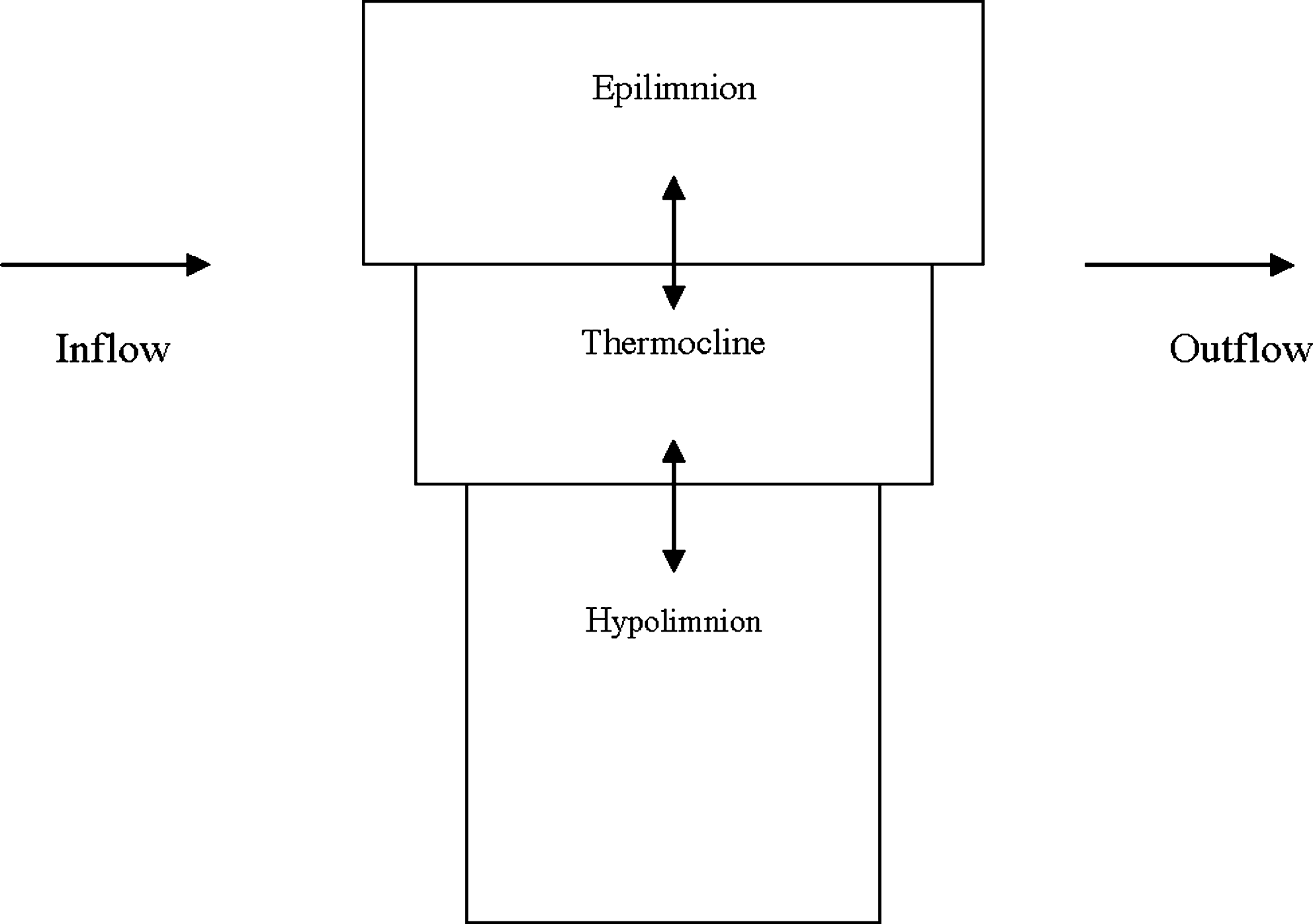
Physical segmentation scheme and transportation.

Mass balance for a substance in the epilimnion, thermocline, and hypolimnion may be written as \documentclass{aastex}\usepackage{amsbsy}\usepackage{amsfonts}\usepackage{amssymb}\usepackage{bm}\usepackage{mathrsfs}\usepackage{pifont}\usepackage{stmaryrd}\usepackage{textcomp}\usepackage{portland, xspace}\usepackage{amsmath, amsxtra}\pagestyle{empty}\DeclareMathSizes{10}{9}{7}{6}\begin{document} \begin{align*} V_1 \frac {\partial c_1} {\partial t} = W_1 (t) - Q_1 c_1 + v_{1 - 2t} A_{2t} (c_2 - c_1) + S_1 \tag{1} \end{align*} \end{document} \documentclass{aastex}\usepackage{amsbsy}\usepackage{amsfonts}\usepackage{amssymb}\usepackage{bm}\usepackage{mathrsfs}\usepackage{pifont}\usepackage{stmaryrd}\usepackage{textcomp}\usepackage{portland, xspace}\usepackage{amsmath, amsxtra}\pagestyle{empty}\DeclareMathSizes{10}{9}{7}{6}\begin{document} \begin{align*} V_2 \frac {\partial c_2} {\partial t} = W_2 (t) - Q_2 c_2 + v_{1 - 2t} A_{2t} (c_1 - c_2) + v_{2 - 3t} A_{3t} (c_3 - c_2) + S_2 \tag{2} \end{align*} \end{document} \documentclass{aastex}\usepackage{amsbsy}\usepackage{amsfonts}\usepackage{amssymb}\usepackage{bm}\usepackage{mathrsfs}\usepackage{pifont}\usepackage{stmaryrd}\usepackage{textcomp}\usepackage{portland, xspace}\usepackage{amsmath, amsxtra}\pagestyle{empty}\DeclareMathSizes{10}{9}{7}{6}\begin{document} \begin{align*} V_3 \frac {\partial c_3} {\partial t} = W_3 (t) - Q_3 c_3 + v_{2 - 3t} A_{3t} (c_2 - c_3) + S_3 \tag{3} \end{align*} \end{document}

where V, c, and t refer to volume, concentration, and time, respectively. W(t), Q, v_t, A_jt, and S_j define loading, outflow, thermocline transfer coefficient, area of layer j, and source or sink terms in layer j, respectively (Chapra, 1997).

Kinetic segmentation

The SD eutrophication model as a simple physical segmentation model consists of 10 state variables. Mass balance equations are written for each state variable for every layer. All equations are developed for a generic layer. Thus they can be applied to the epilimnion, hypolimnion, and/or thermocline layers. The settling term is applied strictly to the hypolimnion, which receives settling gains from the epilimnion or thermocline.

Model formulations

Reservoir volume

Reservoir volume is one of the most important elements in model formulation. Reservoir outflow consists of release for domestic and agricultural uses and evaporation. Reservoir elevation is a function of the reservoir volume, and is calculated based on the storage-elevation curve. The depths of the layers vary with time and are explicitly defined based on the gradient of the temperature field. During the stratified period, the thermocline was defined as the middle layer; other times, only two layers were assumed to reproduce patterns of incomplete mixing in the reservoir. Figure 2 shows the relationships between the hydrological and geometrical elements of the reservoir in the form of a stock-flow diagram.

FIG. 2.

Hydrological and geometrical elements in a stock-flow diagram for reservoir volume feedback loops.

Food chain of phytoplankton

Algae grow as a function of temperature, nutrients, and solar radiation. Sinks include respiration/excretion, grazing, and settling losses. The governing equation for algal biomass considers phytoplankton production and losses due to mortality, settling, and herbivorous zooplankton grazing (Chapra, 1997). The inorganic carbon required for algal growth is assumed to be in excess and thus is not considered by the model. Algae growth rate can be calculated as \documentclass{aastex}\usepackage{amsbsy}\usepackage{amsfonts}\usepackage{amssymb}\usepackage{bm}\usepackage{mathrsfs}\usepackage{pifont}\usepackage{stmaryrd}\usepackage{textcomp}\usepackage{portland, xspace}\usepackage{amsmath, amsxtra}\pagestyle{empty}\DeclareMathSizes{10}{9}{7}{6}\begin{document} \begin{align*} AG (T, n_t, P_s, I) & = AG^{20 \circ C} Min \left( \frac {n_t} {n_t + K_{sn}}, \frac {p_s} {p_s + K_{sp}} \right) \\ & \quad \times 2.718 \times f \times (e^{- \alpha_1} - e^{- \alpha_0}) / (K_eH) \tag{4} \end{align*} \end{document} \documentclass{aastex}\usepackage{amsbsy}\usepackage{amsfonts}\usepackage{amssymb}\usepackage{bm}\usepackage{mathrsfs}\usepackage{pifont}\usepackage{stmaryrd}\usepackage{textcomp}\usepackage{portland, xspace}\usepackage{amsmath, amsxtra}\pagestyle{empty}\DeclareMathSizes{10}{9}{7}{6}\begin{document} \begin{align*} \alpha_1 = \frac {I_a} {I_s} e^{- H_1} \tag{5} \end{align*} \end{document} \documentclass{aastex}\usepackage{amsbsy}\usepackage{amsfonts}\usepackage{amssymb}\usepackage{bm}\usepackage{mathrsfs}\usepackage{pifont}\usepackage{stmaryrd}\usepackage{textcomp}\usepackage{portland, xspace}\usepackage{amsmath, amsxtra}\pagestyle{empty}\DeclareMathSizes{10}{9}{7}{6}\begin{document} \begin{align*} \alpha_0 = \frac {I_a} {I_s} e^{- H_2} \tag{6} \end{align*} \end{document} \documentclass{aastex}\usepackage{amsbsy}\usepackage{amsfonts}\usepackage{amssymb}\usepackage{bm}\usepackage{mathrsfs}\usepackage{pifont}\usepackage{stmaryrd}\usepackage{textcomp}\usepackage{portland, xspace}\usepackage{amsmath, amsxtra}\pagestyle{empty}\DeclareMathSizes{10}{9}{7}{6}\begin{document} \begin{align*} H = H_1 - H_2 \tag{7} \end{align*} \end{document} \documentclass{aastex}\usepackage{amsbsy}\usepackage{amsfonts}\usepackage{amssymb}\usepackage{bm}\usepackage{mathrsfs}\usepackage{pifont}\usepackage{stmaryrd}\usepackage{textcomp}\usepackage{portland, xspace}\usepackage{amsmath, amsxtra}\pagestyle{empty}\DeclareMathSizes{10}{9}{7}{6}\begin{document} \begin{align*} K_e = K_e^{\prime} + 0.0088a + 0.054a^{2/3} \tag{8} \end{align*} \end{document}

where K_e is the extinction coefficient, α₁ and α₀ are the light attenuation factor at the upper and lower depths of the layers and H₁ and H₂ are the depths of the top and bottom of a layer, respectively, a is algae concentration, n_t and p_s are nitrogen and phosphorus concentrations, respectively (Chapra, 1997). Rate of change of algae concentration in the hypolimnion may now be estimated as (Chapra, 1997) \documentclass{aastex}\usepackage{amsbsy}\usepackage{amsfonts}\usepackage{amssymb}\usepackage{bm}\usepackage{mathrsfs}\usepackage{pifont}\usepackage{stmaryrd}\usepackage{textcomp}\usepackage{portland, xspace}\usepackage{amsmath, amsxtra}\pagestyle{empty}\DeclareMathSizes{10}{9}{7}{6}\begin{document} \begin{align*} V \frac {\partial a} {\partial t} = AG (T, n_t, p_s, I) V_a - k_{ra} (T) V_a - C_{gh} (T, a, z_h) V_a + v_a A_ta_u - v_a A_t a \tag{9} \end{align*} \end{document} \documentclass{aastex}\usepackage{amsbsy}\usepackage{amsfonts}\usepackage{amssymb}\usepackage{bm}\usepackage{mathrsfs}\usepackage{pifont}\usepackage{stmaryrd}\usepackage{textcomp}\usepackage{portland, xspace}\usepackage{amsmath, amsxtra}\pagestyle{empty}\DeclareMathSizes{10}{9}{7}{6}\begin{document} \begin{align*} C_{gh} (T, a, z_h) = \frac {a} {a + k_{sa}} C_{gh} \theta^{T - 20} z_h \tag{10} \end{align*} \end{document}

Figure 3 shows the complete feedback loops for phytoplankton. As shown in the figure, nitrate, ammonia, and soluble reactive phosphorus (SRP) affect phytoplankton concentration in the system. In any layer, there are the same feedback and relations between phytoplankton concentrations and other water quality variables.

FIG. 3.

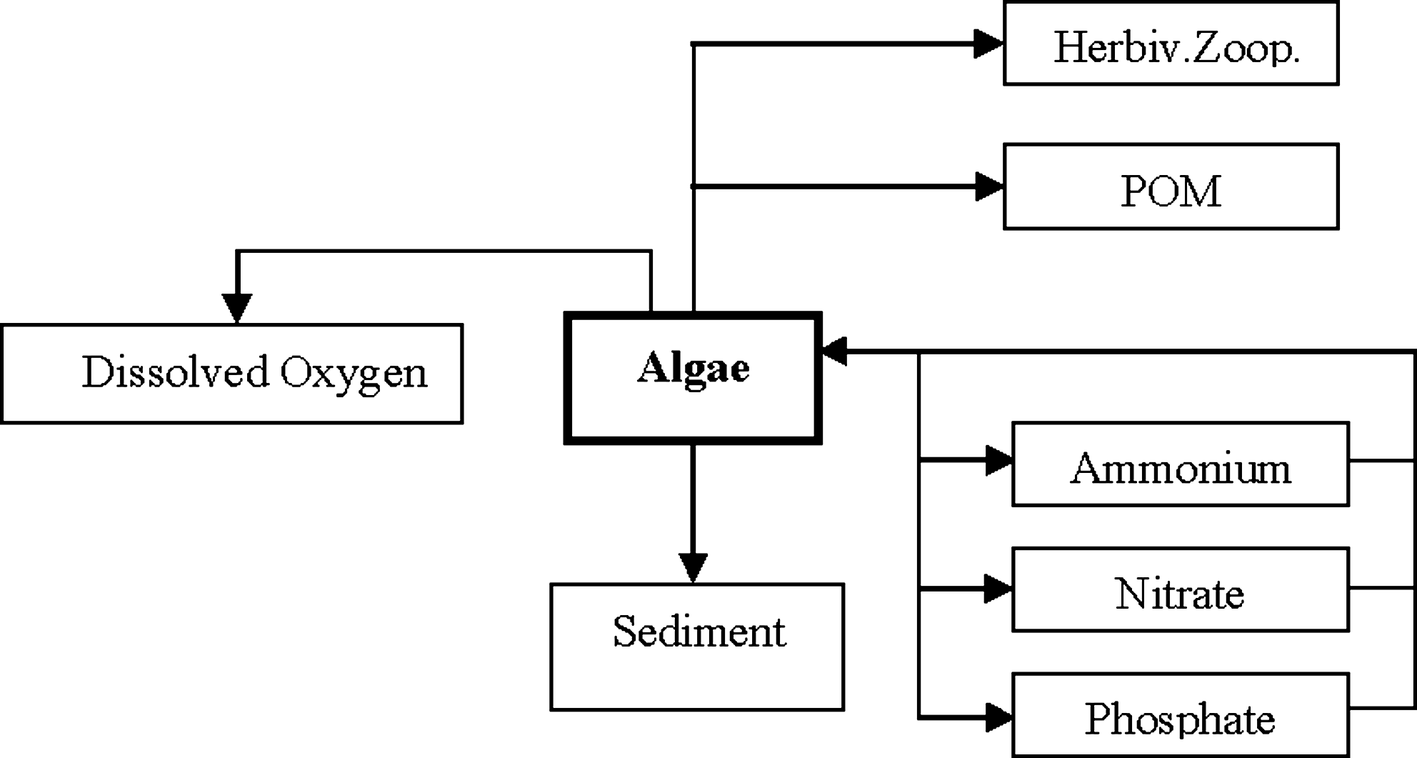
Feedback of phytoplankton stock with other water quality constituents.

Food chain of zooplankton

Part of the consumed algae is converted into herbivorous zooplankton. The herbivores are depleted by carnivore grazing and respiration/excretion losses (Chapra, 1997; Cole and Wells, 2008): \documentclass{aastex}\usepackage{amsbsy}\usepackage{amsfonts}\usepackage{amssymb}\usepackage{bm}\usepackage{mathrsfs}\usepackage{pifont}\usepackage{stmaryrd}\usepackage{textcomp}\usepackage{portland, xspace}\usepackage{amsmath, amsxtra}\pagestyle{empty}\DeclareMathSizes{10}{9}{7}{6}\begin{document} \begin{align*} V \frac {\partial z_h} {\partial t} = \varepsilon_h C_{gh} (T, a, z_h) V_a - C_{gc} (T, z_c) {V}_{{z}_{h}} - k_{rh} (T) {V}_{{z}_{h}} \tag {11}\end{align*} \end{document}

The carnivores are depleted by respiration/excretion losses and a first-order death due to grazing by organisms higher on the food chain (Chapra, 1997): \documentclass{aastex}\usepackage{amsbsy}\usepackage{amsfonts}\usepackage{amssymb}\usepackage{bm}\usepackage{mathrsfs}\usepackage{pifont}\usepackage{stmaryrd}\usepackage{textcomp}\usepackage{portland, xspace}\usepackage{amsmath, amsxtra}\pagestyle{empty}\DeclareMathSizes{10}{9}{7}{6}\begin{document} \begin{align*} V \frac {\partial z_c} {\partial t} = \varepsilon_c C_{gc} (T, z_c) {V}_{{z}_{h}} - k_{rc} (T) {V}_{{z}_{c}} - k_{dc} (T) {V}_{{z}_{c}} \tag {12}\end{align*} \end{document}

Organic matter

Organic matter is divided into particulate and dissolved fractions. Inefficient grazing along carnivore death results in gains to the POM pool (Chapra, 1997; Arhonditsis and Brett, 2005a, 2005b; Cole and Wells, 2008): \documentclass{aastex}\usepackage{amsbsy}\usepackage{amsfonts}\usepackage{amssymb}\usepackage{bm}\usepackage{mathrsfs}\usepackage{pifont}\usepackage{stmaryrd}\usepackage{textcomp}\usepackage{portland, xspace}\usepackage{amsmath, amsxtra}\pagestyle{empty}\DeclareMathSizes{10}{9}{7}{6}\begin{document} \begin{align*} & V \frac {\partial c_{po}} {\partial t} = (1 - \varepsilon_h) C_{gh} (T, a, z_h) V_a + (1 - \varepsilon_c) C_{gc} (T, z_c) {V}_{{z}_{h}} \\& + k_{dc} (T) {V}_{{z}_{c}} - k_{po} (T) V_{po} + v_{po} A_t c_{pou} - v_{po} A_t c_{po} \tag{13} \end{align*} \end{document}

where c_pou is concentration of POM in the upper layer. DOM is gained via the first-order dissolution reaction and lost by hydrolysis (Chapra, 1997): \documentclass{aastex}\usepackage{amsbsy}\usepackage{amsfonts}\usepackage{amssymb}\usepackage{bm}\usepackage{mathrsfs}\usepackage{pifont}\usepackage{stmaryrd}\usepackage{textcomp}\usepackage{portland, xspace}\usepackage{amsmath, amsxtra}\pagestyle{empty}\DeclareMathSizes{10}{9}{7}{6}\begin{document} \begin{align*} V \frac {\partial c_{do}} {\partial t} = k_{po} (T) V_{po} - k_h (T) V_{do} \tag {14} \end{align*} \end{document}

Nutrients—nitrogen

In the simulated nitrogen cycle, nitrate-nitrite (NO₃) and ammonium (NH₄) are incorporated by the algae. Egestion of excess nitrogen during zooplankton feeding and phytoplankton and zooplankton basal metabolism releases ammonium and organic nitrogen in the water column. A portion of the particulate organic nitrogen is converted into dissolved organic nitrogen (DON). DON is mineralized to NH₄ and made available again to the algae either as NH₄ or as NO₃. In an oxygenated water column, ammonium is oxidized to nitrate through nitrification and its kinetics is modeled as a function of available ammonium, DO, temperature, and light (Cerco and Cole, 1993; Cole and Wells, 2002). \documentclass{aastex}\usepackage{amsbsy}\usepackage{amsfonts}\usepackage{amssymb}\usepackage{bm}\usepackage{mathrsfs}\usepackage{pifont}\usepackage{stmaryrd}\usepackage{textcomp}\usepackage{portland, xspace}\usepackage{amsmath, amsxtra}\pagestyle{empty}\DeclareMathSizes{10}{9}{7}{6}\begin{document} \begin{align*} V \frac {\partial n_a} {\partial t} & = a_{no} k_h (T) V_{do} + a_{na} k_{ra} (T) V_a + a_{no} k_{rh} (T) {V}_{{z}_{h}} \\ & \quad + a_{no} k_{rc} (T) {V}_{{z}_{c}} - F_{am} a_{na} AG (T, n_t, p_s, I) V_a \\ & \quad - k_n (T) V_{na} + K_{\rm NO_x} (T) V_{ni} + a_{no} K_s (T) V_{Sed} \\ & \quad + SOD_{\rm NH_4} \times A_{sed} \tag{15} \end{align*} \end{document} \documentclass{aastex}\usepackage{amsbsy}\usepackage{amsfonts}\usepackage{amssymb}\usepackage{bm}\usepackage{mathrsfs}\usepackage{pifont}\usepackage{stmaryrd}\usepackage{textcomp}\usepackage{portland, xspace}\usepackage{amsmath, amsxtra}\pagestyle{empty}\DeclareMathSizes{10}{9}{7}{6}\begin{document} \begin{align*} F_{am} = \frac {n_a} {n_a + K_{am}} \tag{16} \end{align*} \end{document}

where F_am is the fraction of inorganic nitrogen taken from the ammonia pool by plant uptake, and a_no and a_na are the ratios of nitrogen to organic matter and chlorophyll a (Chlr a), respectively. K_NOx, SOD_NH4, and A_sed are nitrate-nitrogen decay rate, zero-order sediment ammonium release rate, and sediment area, respectively. In this study, the last two terms of equation (15) are considered only in the hypolimnion. Only under anoxic conditions, nitrate is lost through denitrification and zero-order sediment ammonium release occurs.

Nitrate is gained by nitrification and lost via plant uptake (Chapra, 1997) and through denitrification process in anoxic condition (Cole and Wells, 2002): \documentclass{aastex}\usepackage{amsbsy}\usepackage{amsfonts}\usepackage{amssymb}\usepackage{bm}\usepackage{mathrsfs}\usepackage{pifont}\usepackage{stmaryrd}\usepackage{textcomp}\usepackage{portland, xspace}\usepackage{amsmath, amsxtra}\pagestyle{empty}\DeclareMathSizes{10}{9}{7}{6}\begin{document} \begin{align*} V \frac {\partial n_i} {\partial t} = k_n (T) V_{n_a} - (1 - F_{am}) a_{na} AG (T, n_t, p_s, I) V_a - K_{\rm NO_x} (T) {V}_{{n}_{i}} \tag{17} \end{align*} \end{document}

Figures 4 and 5 show the feedback loops of ammonium and nitrate stocks with other stocks.

FIG. 4.

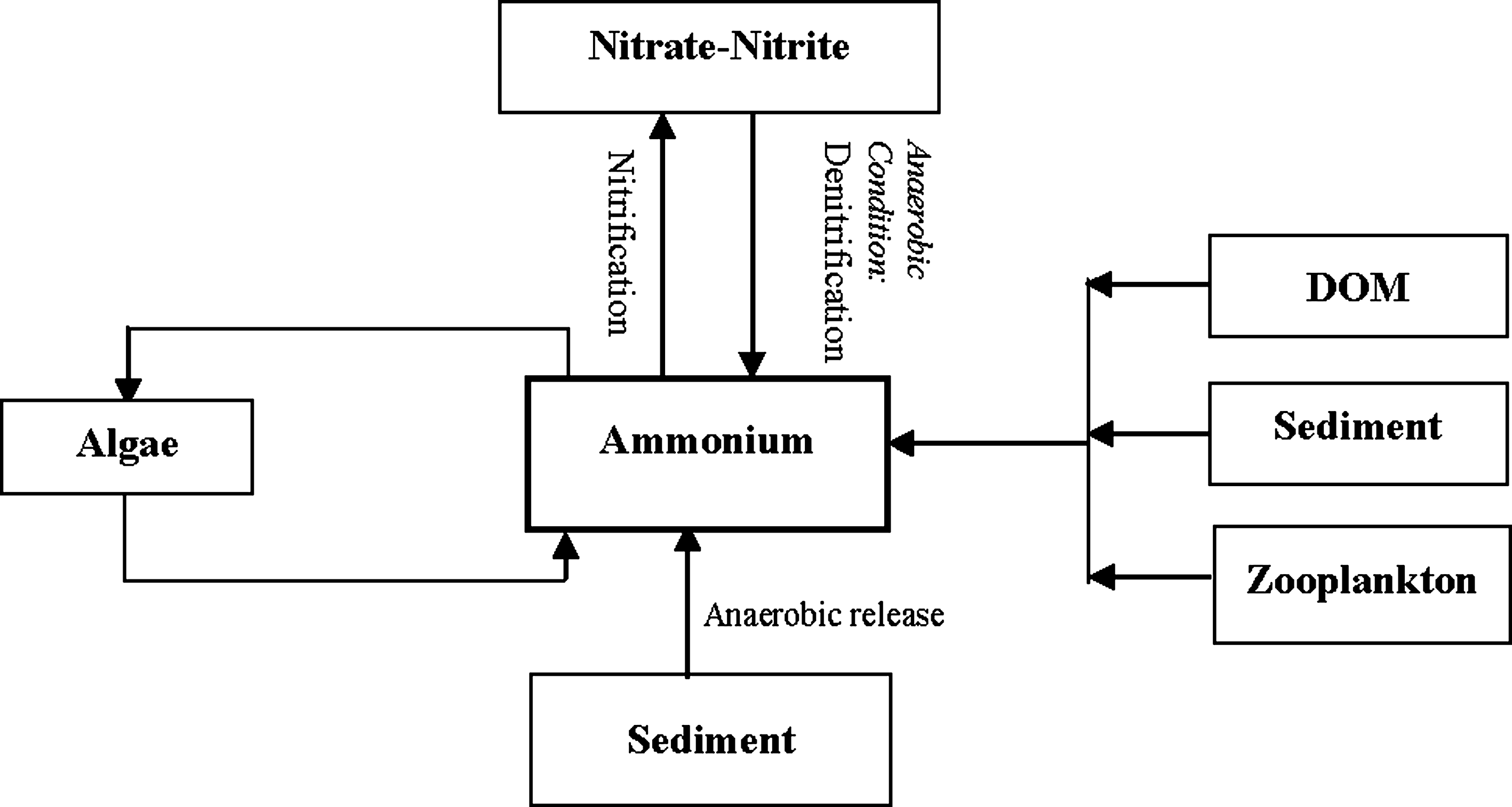
Feedback of ammonium constituent with other water quality constituents.

FIG. 5.

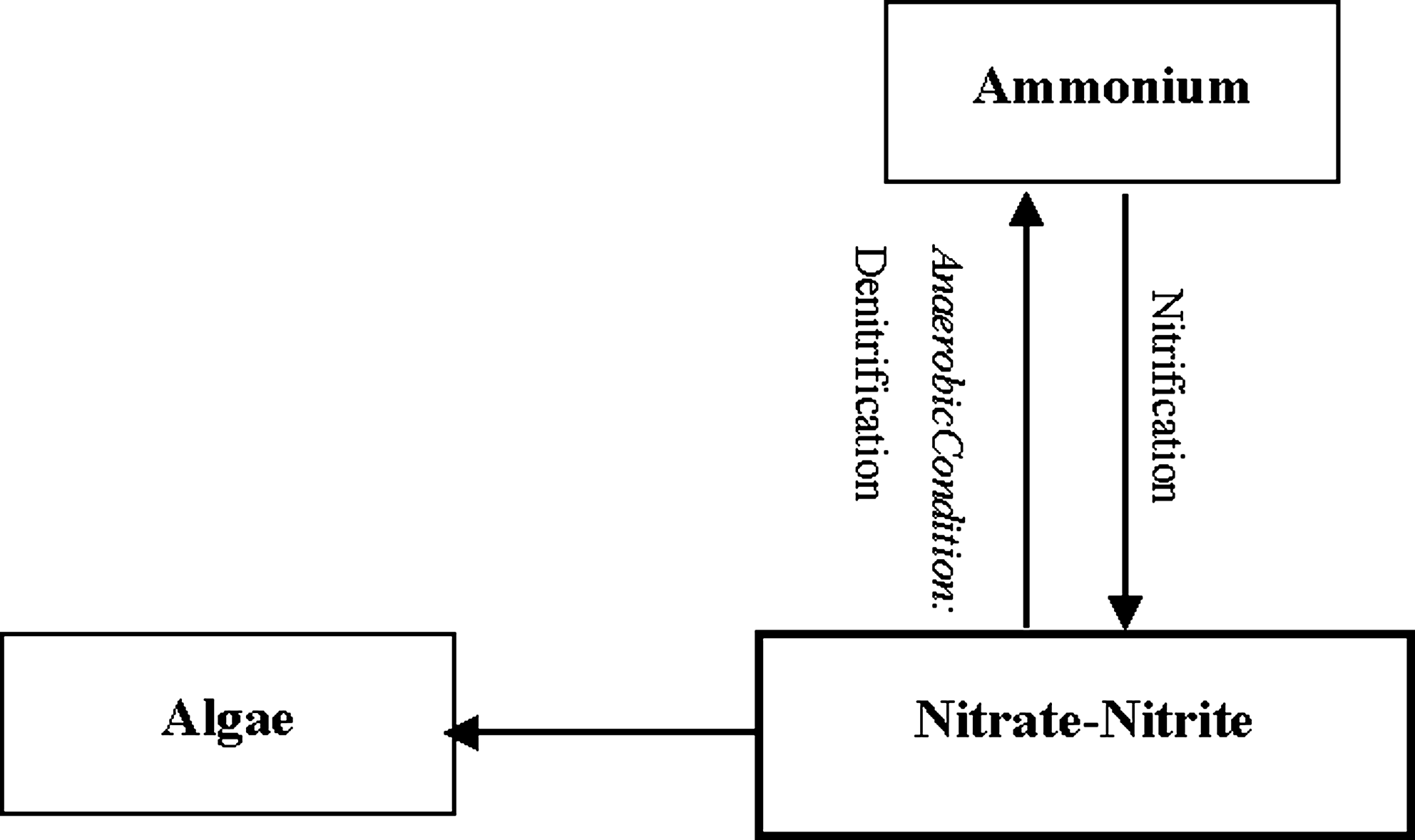
Feedback of nitrate constituent with other water quality constituents.

Nutrients—phosphorus

The phosphorus-loading concept is based on the premise that phosphorus is the primary, controllable limiting nutrient of lake and reservoir eutrophication. Phytoplankton and zooplankton basal metabolism and egestion of excess phosphorus during feeding release phosphate and particulate organic phosphorus. Dissolved organic phosphorus is converted to phosphate through a first-order reaction (Chapra, 1997; Arhonditsis, 2005a, 2005b; Cole and Wells, 2008): \documentclass{aastex}\usepackage{amsbsy}\usepackage{amsfonts}\usepackage{amssymb}\usepackage{bm}\usepackage{mathrsfs}\usepackage{pifont}\usepackage{stmaryrd}\usepackage{textcomp}\usepackage{portland, xspace}\usepackage{amsmath, amsxtra}\pagestyle{empty}\DeclareMathSizes{10}{9}{7}{6}\begin{document} \begin{align*} V \frac{\partial p_s} {\partial t} & = a_{po} k_h (T) {V}_{{c}_{do}} + a_{pa} k_{ra} (T) V_a + a_{po} k_{rh} (T) {V}_{{z}_{h}} \\ & \quad+ a_{po} k_{rc} (T) {V}_{{z}_{c}} - a_{pa} AG (T, n_t, p_s, I) V_a \\ & \quad+ a_{po} K_s (T) V_{sed} + SOD_{\rm PO_4} \times A_{sed} \tag{18} \end{align*} \end{document}

where a_po and a_pa are the ratios of phosphorus to organic matter and Chlr a, respectively. SOD_PO4 is the zero-order anerobic sediment release rate. The feedback of phosphate with other stocks are shown in Fig. 6.

FIG. 6.

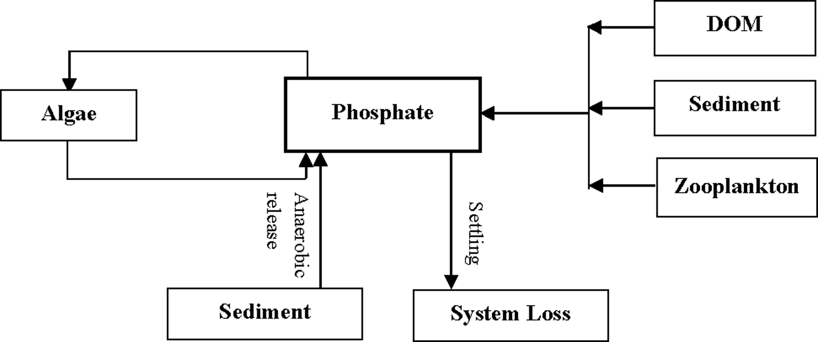
Feedback of phosphate constituent with other water quality constituents.

In this study, the last two terms of Equation (18) are considered only in the hypolimnion layer, and phosphorus zero-order sediment release is allowed to occur only if the overlying water DO concentration is less than a minimum value (anerobic condition) (Cole and Wells, 2002).

Dissolved oxygen

The major sources and sinks of DO in the water column include phytoplankton photosynthesis and respiration, nitrification, decomposition of organic matter in the sediments and water column, denitrification, and atmospheric reaeration. The rate of the latter process is proportional to DO deficit, while DO saturation concentration decreases as temperature increases, based on the empirical formula provided by APHA (1992): \documentclass{aastex}\usepackage{amsbsy}\usepackage{amsfonts}\usepackage{amssymb}\usepackage{bm}\usepackage{mathrsfs}\usepackage{pifont}\usepackage{stmaryrd}\usepackage{textcomp}\usepackage{portland, xspace}\usepackage{amsmath, amsxtra}\pagestyle{empty}\DeclareMathSizes{10}{9}{7}{6}\begin{document} \begin{align*} V \frac {\partial O} {\partial t} &= (AG (T, n_t, p_s, I) - k_{ra}) V_a \gamma_{OM} + A_{surface} .K_L (O_{sat} - O) \\ & \quad + K_{NO_3} (T) {V}_{{n}_{i}} \gamma_{\rm NH_4} - k_{po} (T) {V}_{{c}_{po}} \gamma_{OM} - k_n V_{na} \gamma_{\rm NH_4} \\ & \quad - \gamma_{OM} K_s (T) V_{sed} - SOD (T) \times A_{sed} \tag{19}\end{align*} \end{document}

where O_sat is the saturation DO concentration and SOD is the zero-order bottom sediment oxygen demand, which is considered in the hypolimnion.

Total suspended solids (TSS)

In this research, TSS is modeled in the simplest manner. Mass balance equations are written for the suspended solids in the epilimnion, thermocline, and hypolimnion. Then a given sediment layer is assumed to be placed in the hypolimnion. The mass balance equation in the hypolimnion layer is as below (Chapra, 1997): \documentclass{aastex}\usepackage{amsbsy}\usepackage{amsfonts}\usepackage{amssymb}\usepackage{bm}\usepackage{mathrsfs}\usepackage{pifont}\usepackage{stmaryrd}\usepackage{textcomp}\usepackage{portland, xspace}\usepackage{amsmath, amsxtra}\pagestyle{empty}\DeclareMathSizes{10}{9}{7}{6}\begin{document} \begin{align*} V_3 \frac {\partial c_{3_{TSS}}} {\partial t} & = W_{3_{TSS}} (t) - Q_3 c_{3_{TSS}} - v_{st_{ss}} A_{sed} c_{3_{TSS}} + v_{st_{ss}} A_{3t} c_{2_{TSS}} \\ & \quad + v_{2}-{3t} A_{3t} (c_{2_{TSS}} - c_{3_{TSS}}) + v_r A_{sed} c_{sed} \tag {20} \end{align*} \end{document}

The last term in Equation (20) refers to sediment resuspension, which is considered only in the hypolimnion layer.

Simulation Model

Understanding the system components and its boundaries, identifying the key variables, defining the mathematical relationship among physical processes or variables, mapping the structure of the model, and simulating the model for understanding its behavior are the major steps in applying the SD approach (Simonovic, 2009). These steps are applied in this research to develop the SD eutrophication model.

The SD eutrophication model is programmed in Vensim (Ventana Systems, 2009) environment, where words are connected with arrows; relationships among system variables are entered as mathematical formulations and recorded as causal connections. This information is used by the equation editor to help form a complete simulation model. A simple and flexible way of building simulation models from causal loop or stock and flow diagrams is provided in the Vensim environment.

The purpose of the study is to develop a SD object-oriented reservoir eutrophication model and assess its performance by using field data and/or results of the CE-QUAL-W2 model. As mentioned earlier, the developed model divided the reservoir into three layers. During cold seasons, temperature gradient in the layers is low, and so the thermocline layer is eliminated and there are only two layers.

Input data include the reservoir elevation-storage-area curve, daily evaporation losses, measured temperature in the three main layers of the reservoir, initial water quality concentration in the three main layers, initial water surface elevation, daily water inflow rate, water quality inflow rate, hypolimnetic sediment concentration, and daily water outflows.

The hydrological, geometrical, water temperature, and water quality data for model calibration and performance evaluation were provided by the Iran Water and Power Company Karkheh reservoir Monitoring Program (Iran WPC, 2006). The water quality monitoring program conducted 12 surveys per year at approximately four stations in the reservoir during 2003 to 2006. The data were collected at a variety of frequencies varying from daily to monthly.

Parameters and coefficients that affect the concentration of PO₄, NH₄, NO₃, DO, and Chlr a were determined in a detailed calibration process. Other simulated constituents included TSS, DOM, and POM. Numerous model runs were conducted to calibrate the SD eutrophication model parameters, which were determined by trial and error method through model simulation. Following each run, the water levels and water quality variables in each layer were carefully studied. Modifications to the model parameters were made to match the water quality variables with the observed values during calibration period. The calibrated kinetic coefficients and constants for water quality simulation for the Karkheh Reservoir are listed in Table 1. Generally, they are consistent with the literature values.

Table 1.

System Dynamic Eutrophication Model Parameter Values (Coefficients) for the Karkheh Reservoir

Name of parameter		Value	Reference value	Unit
AG_20°C	Algae growth rate at 20°C	2.4	2^a	day⁻¹
K_sn	Algal half-saturation for nitrogen limited growth	0.15	0.012–0.923 NO₃^b	mg N/L
K_sp	Algal half-saturation for phosphorus limited growth	0.0126	0.002–0.475^b	mg P/L
f	Photoperiod	0.45	0.5^a
I_s	Optimal light level	380	100–400^a	Ly/day
I_a	Average day light intensity	270	500^a	Ly/day
\documentclass{aastex}\usepackage{amsbsy}\usepackage{amsfonts}\usepackage{amssymb}\usepackage{bm}\usepackage{mathrsfs}\usepackage{pifont}\usepackage{stmaryrd}\usepackage{textcomp}\usepackage{portland, xspace}\usepackage{amsmath, amsxtra}\pagestyle{empty}\DeclareMathSizes{10}{9}{7}{6}\begin{document} $$K_e^{\prime}$$ \end{document}	Light extinction coefficient due to factors other than phytoplankton	0.837	0.3^a	m⁻¹
v_a	Phytoplankton settling velocity	0.09	0.08–1.9^a	m/day
k_ra	Losses due to respiration and excretion	0.024	0.025^a	day⁻¹
C_gh	Herbivorous grazing losses	0.8	1.5^c	day⁻¹
k_sa	Herbivorous zooplankton saturation for algae limited growth	0.8	0.01^a	mg Chlr a/L
ɛ_h	Herbivorous zooplankton grazing efficiency	0.6	0.7^a
C_gc	Carnivorous grazing losses	0.3	1.5	day⁻¹
k_rh	Herbivorous zooplankton respiration/excretion rate	0.12	0.1^a	day⁻¹
ɛ_c	Carnivore zooplankton grazing efficiency	0.7	0.7^a
k_rc	Carnivorous zooplankton respiration/excretion rate	0.075	0.04^a	day⁻¹
k_dc	Carnivore first-order death	0.075	0.04^a	day⁻¹
k_po	Dissolution rate of particulate organic matter	0.1	0.1^a	day⁻¹
v_po	Settling rate of particulate organic matter	0.1	0.2^a	m/day
k_h	Hydrolysis rate of dissolved organic matter	0.075	0.075^a	day⁻¹
k_n	Nitrification rate	0.095	0.1^a	day⁻¹
γ_OM	Oxygen stoichiometric coefficients for organic matter	1.4	1.4^c	g O₂/g OM
\documentclass{aastex}\usepackage{amsbsy}\usepackage{amsfonts}\usepackage{amssymb}\usepackage{bm}\usepackage{mathrsfs}\usepackage{pifont}\usepackage{stmaryrd}\usepackage{textcomp}\usepackage{portland, xspace}\usepackage{amsmath, amsxtra}\pagestyle{empty}\DeclareMathSizes{10}{9}{7}{6}\begin{document} $$\gamma_{NH_4}$$ \end{document}	Oxygen stoichiometric coefficients for nitrification/denitrification	4.57	4.57^c	g O₂/g N
\documentclass{aastex}\usepackage{amsbsy}\usepackage{amsfonts}\usepackage{amssymb}\usepackage{bm}\usepackage{mathrsfs}\usepackage{pifont}\usepackage{stmaryrd}\usepackage{textcomp}\usepackage{portland, xspace}\usepackage{amsmath, amsxtra}\pagestyle{empty}\DeclareMathSizes{10}{9}{7}{6}\begin{document} $$v_{st_ss}$$ \end{document}	TSS settling velocity	0.32	0.3–1^a	m/day
v_r	Sediment resuspension velocity	0.001	0.003^a	mm/day
K_s	First-order sediment decay rate	0.025	0.1^c	day⁻¹
K_am	Half-saturation constant for ammonium preference	0.015	0.05^a	mg N/L
K_L	Interfacial exchange rate for oxygen	2.78	∼2.5^c,d	m/day

Chapra (1997).

Tufford and McKellar (1999).

Cole and Wells (2002).

Based on Kanwisher's equation (1963).

Calibration and verification of water elevation and water quality relied upon vertical profile data from the reservoir and CE-QUAL-W2 model results. In this study, the Karkheh Reservoir system model was calibrated from May 17, 2005 to July 22, 2006 and it was verified during July 2, 2003 to May 30, 2004.

The eutrophication behavior of the reservoir, unfolding over time, which shows how the process arose and how it might evolve in the future, has been characterized through SD eutrophication modeling. The relations are expressed as a series of 30 differential equations and state variables for the rates of change of phytoplankton, herbivorous zooplankton, carnivorous zooplankton, POM, DOM, ammonium, nitrogen, phosphorus, TSS, and DO. The inflow and outflow volumes have been entered daily. By using the kinetic interactions from Equations (4 )–(20), one can write Equations (1 )–(3) for each of the 10 state variables. The resulting 30 ordinary differential equations can be integrated simultaneously using a numerical method.

Vensim software solves a set of differential equations through numerical integration according to several techniques available in it, such as Euler's method or second-order and fourth-order Runge–Kutta method. In this study, fourth-order Runge–Kutta technique integrated with automatic adjustment of the step size to ensure accuracy is implemented.

Study Site

In 1999 the Karkheh Reservoir was constructed on the Karkheh River, one of the most important rivers in Iran. The Karkheh River is located in the southwest region of Iran in the mountainous and plain surroundings and receives runoff from a catchment area of 50,000 km². The latitude and longitude coordinates for the reservoir are 32°50′ and 48°15′, respectively. The Karkheh Reservoir has a surface area of 162 km², extends to 64 km, and has a storage capacity of about 5×10⁹ m³. The elevation-area-storage relationships for the Karkheh Reservoir are presented in Table 2.

Table 2.

Elevation-Area-Storage Relationship in Karkheh Reservoir

Elevation (masl.)	Area (km ² )	Volume (MCM)
113	0	0
115	0.14	0.14
120	0.78	2.45
130	3.12	21.94
140	7.91	77.09
150	15.41	193.7
160	25.29	397.11
170	39.03	715.55
180	55.16	1188.03
190	76.03	1848.53
200	102.25	2733.2
210	128.11	3886.1
220	162.47	5346.8

MASL, Meter above Sea Level; MCM, Million Cube Meter.

The average and maximum depths of the reservoir are 61.8 and 117 m, respectively. The Karkheh Reservoir is a multipurpose hydraulic project built to provide water for irrigation, drinking, and power generation. The geographic location of the Karkheh basin in Iran and its relative position with respect to neighboring countries is presented in Fig. 7.

FIG. 7.

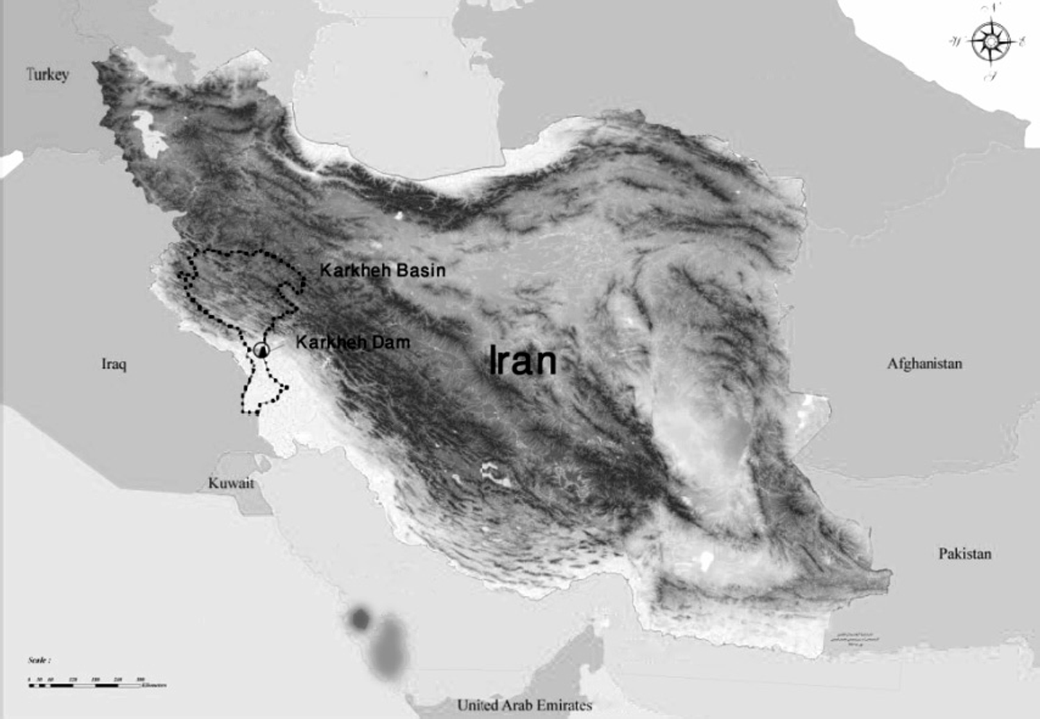
Geographic location of Karkheh basin in Iran and the relative position with respect to neighboring countries.

Model Results

Reservoir volume and water surface elevation

Collecting and setting up the adjustable geometrical characteristic and evaporation losses have been done to maximize the fit to the observed values for reservoir water elevations. The results of water surface elevation modeling with the proposed SD eutrophication model and CE-QUAL-W2 (Afshar and Saadatpour, 2009) are presented in Fig. 8. Both the maximum error and the average error with the two models fall within acceptable ranges for the Karkheh Reservoir with very large inflow.

FIG. 8.

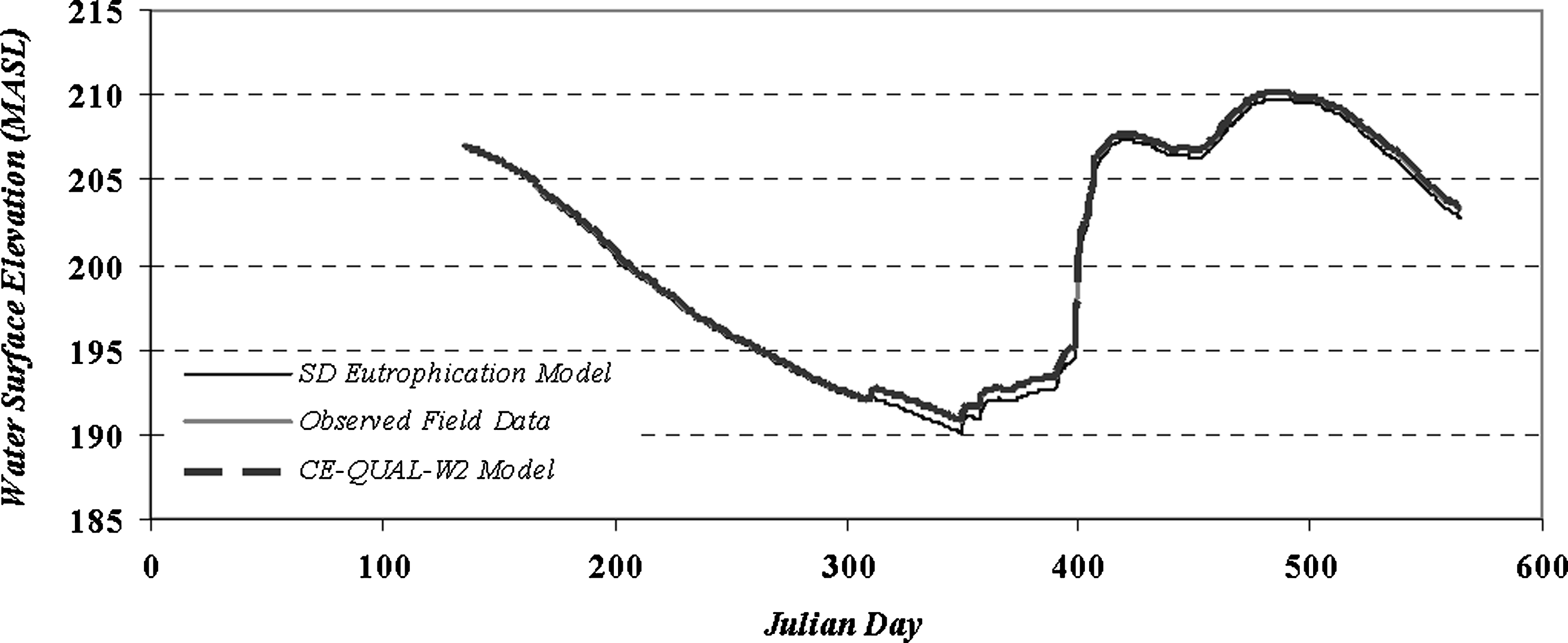
Comparison of water surface elevation of system dynamic (SD) eutrophication model results with CE-QUAL-W2 model results and observed field data.

Water quality variables

Based on Equations (4 )–(20), causal feedback loops were developed for three segmented layers of epilimnion, thermocline, and hypolimnion. Results of the CE-QUAL-W2 model were longitudinal and depth averaged over the epilimnion, thermocline, and hypolimnion to be comparable with those of the SD eutrophication model. Any water quality stock in one layer is related to its next layer or layers through the process of diffusion.

Algal biomass predicted by the SD eutrophication model is compared with the available Chlr a data and those of CE-QUAL-W2 model in the three layers (Fig. 9).

FIG. 9.

Chlr a concentration in (a) epilimnion layer, (b) thermocline layer, and (c) hypolimnion layer.

As is clear from Fig. 9, in the cold season (December to March; Julian day 340 to 430) the reservoir experiences low growth, while the highest growth is expected during warmer seasons. With regard to decreasing the light and temperature (during the warm seasons) in the water column (deep depths), algae growth rate is limited in the lower layers. In the cold seasons, because of high diffusion rate in the epilimnion and hypolimnion layers, Chlr a concentration in the reservoir is homogeneous and the hypolimnion layer experiences higher Chlr a concentration than during warmer seasons.

Nutrient concentrations in the epilimnion show a consistent seasonal pattern through the simulation period. Phosphate and ammonium concentrations are highest during the late winter and early spring due to low algae uptake, and lowest during the late spring and early summer due to high algae uptake. As mentioned earlier, sediment contribution of phosphorus and/or ammonium to hypolimnion layer is modeled as a zero and first-order process [Eqs. (15) and (18)]. In this research, the high concentration of phosphate and/or ammonium in the hypolimnion layer is due to first-order sediment release rate (Figs. 10 and 11). Zero-order phosphate and ammonium releases do not occur when DO concentrations are above a minimum value (Cole and Wells, 2002).

FIG. 10.

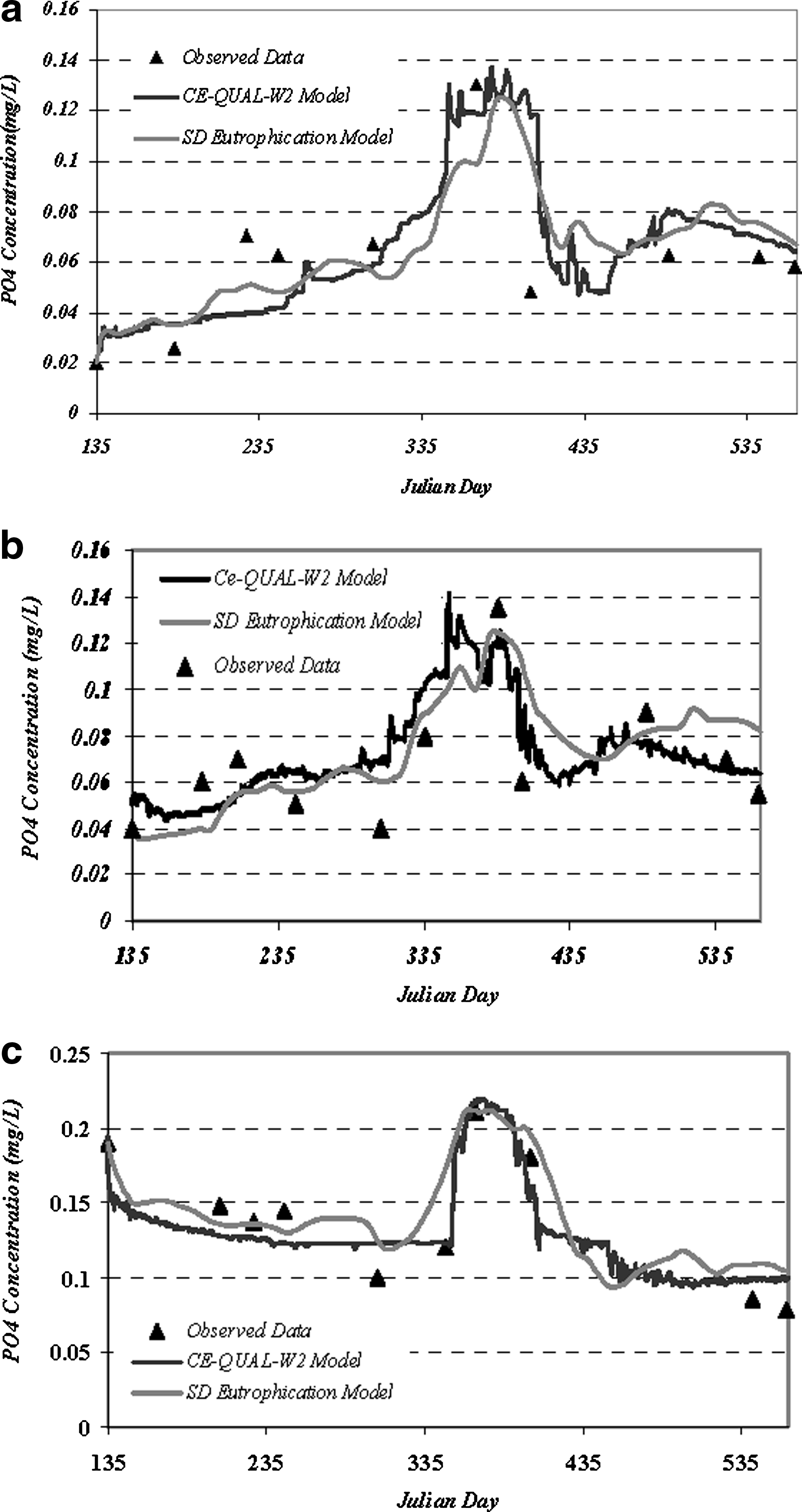
PO₄-P concentration in (a) epilimnion layer, (b) thermocline layer, and (c) hypolimnion layer.

FIG. 11.

NH₄-N concentration in (a) epilimnion layer, (b) thermocline layer, and (c) hypolimnion layer.

During warmer seasons, concentration of nitrate in the epilimnion layer remains low partially because of algae uptake and low ammonium concentration, and partially because no new inputs occur (Fig. 12). During December to March, high hypolimnetic ammonium concentration and low algae uptake lead to high hypolimnetic nitrate concentration.

FIG. 12.

NO₃-N concentration in (a) epilimnion layer, (b) thermocline layer, and (c) hypolimnion layer.

Concentrations of DO in the layers are shown in Fig. 13. DO concentration in the epilimnion is higher than in other layers, possibly related to the interfacial oxygen exchange due to reaeration process in the water surface and higher sediment oxygen demand in the lower layers. During December to March, as the reservoir surface would be cold, oxygen solubility increases and the epilimnetic concentrations increase due to high reaeration rate (APHA, 1992). In this period, due to high diffusion rate in the epilimnion and hypolimnion layers, levels of DO in the reservoir are high and homogeneous.

FIG. 13.

Dissolved oxygen concentration in (a) epilimnion layer, (b) thermocline layer, and (c) hypolimnion layer.

Predicted values for the SD eutrophication model are satisfactory compared with measured field data and/or CE-QUAL-W2 model results. The proposed model was verified during May 20, 2003 to July 4, 2004. Model outputs are compared with the available water quality data and CE-QUAL-W2 model results (Mohamadi, 2004). Considering the temporal and spatial variations in quality parameters throughout the reservoir, the accuracy of the model is shown to be satisfactory for model projection and for the evaluation of future management strategies. Mean absolute errors (MAE) for the constituents with the available field data and CE-QUAL-W2 model results do not exceed 18%. MAE for nitrate is less than 14% and for phosphorus, ammonium, and DO are less than 18% for the verification period.

Figure 14 illustrates the variation in phytoplankton, herbivorous zooplankton, and carnivorous zooplankton concentrations during the simulation period. The results indicate that predator-prey interactions are taking place, with the peak of the algae, herbivores, and carnivores occurring approximately on Julian days 254, 328, and 361, respectively.

FIG. 14.

Phytoplankton (algae), herbivorous zooplankton, and carnivorous zooplankton concentrations in the epilimnion layer.

After initiation of the spring bloom, herbivorous zooplankton populations respond progressively but do not exert a significant grazing pressure until November, as can be inferred by the maximum grazing rate values. However, as the epilimnetic food concentration (phytoplankton) increases in September, an abrupt increase in the grazing coefficient occurs. From this point, the system is dominated by herbivorous zooplankton grazing and consequently undergoes prey-predator oscillations. On the other hand, high herbivorous zooplankton concentration in November increases food availability for carnivorous zooplankton. So, at relatively high food concentrations, carnivorous zooplankton grazing rate increases.

The SD eutrophication model is developed for purposes of rapid, interactive scenario evaluation. The developed model took less than 1 s to run on a PC with 3 GHz Pentium IV processor and 1.98 GB Ram, Dual Core, whereas the two-dimensional hydrodynamic and process-based water quality model (CE-QUAL-W2) run time is about 6 min for the same simulation period. The semi-distributed SD eutrophication model thus provides a legitimate proxy to the more complex CE-QUAL-W2 models for rapid scenario evaluation of a wide range of alternative futures.

Nutrient Load Reduction/Increase Scenarios

Increased loading from upstream watershed in the Karkheh River basin makes it necessary to assess different scenarios in order to predict how the system will respond to changes in external forces such as nutrient loading. At the same time, the basic goal of this SD eutrophication model is to support management planners and decision-makers in testing the resilience of the Karkheh Reservoir under various management scenarios in the preliminary stages.

The system is simulated for four different scenarios: (1) reference scenario (current state), (2) reducing/increasing nitrate and ammonium loads, (3) reducing/increasing phosphorus loads, and (4) reducing/increasing total nutrient loads originating in the Karkheh territory.

As presented in Fig. 15, any changes in phosphorus input into the reservoir significantly affect the average Chlr a concentration. In fact, concentration of Chlr a within the reservoir is highly dependent on the phosphorus concentration in the inflowing water. To further test this hypothesis, different concentrations of nitrate and ammonium in the inflow were examined, keeping the phosphorus concentration unchanged. Resulting variations in Chlr a concentration were very minor. It may be concluded that the reservoir is quite sensitive to the phosphorus load.

FIG. 15.

Chlr a concentration, scenarios increasing/decreasing phosphorus load, time series.

Concluding Remarks

Water quality is highly important in reservoir management for a number of reasons. Existing reservoirs are being subjected to intense multi-objective demands on limited resources, and thus, water use attracts more attention causing water quality to draw closer scrutiny.

The proposed SD eutrophication model considers feedback and interactive loops between phytoplankton, herbivorous zooplankton, carnivorous zooplankton, POM, DOM, ammonium, nitrate, phosphorus, TSS, and DO. The model divides the reservoir into three layers and is expressed as a series of 30 differential equations for 10 state variables in the layers. Due to rapid, non-resource-intensive, but low-resolution outputs of the developed model, it is most appropriate at the planning/reconnaissance level of water resources decision makings or in low controversy situations.

The SD eutrophication model reproduces the epilimnion, thermocline, and hypolimnion temporal patterns of the system, and the results compare well with the simulated and observed monthly data and also with the results of the CE-QUAL-W2 model during calibration and verification periods.

The verified SD eutrophication model was used to assess the impact of nutrient load in the Karkheh watershed on the eutrophication due to stakeholders' contributions. It was concluded that in the Karkheh Reservoir, phosphor is the limiting factor for algae growth and primary productivity.

Finally, this study emphasizes the need for integrating the SD eutrophication model with a hydrodynamic model having a fine vertical resolution. Eutrophication through SD modeling can be extended to other water bodies such as elongated lakes, streams, and estuaries with additional nutrients and food chain components.

Footnotes

Author Disclosure Statement

No competing financial interests exist.

References

Afshar

, Saadatpour

2009. Reservoir eutrophication modelling, sensitivity analysis, and assessment: Application to Karkheh Reservoir, Iran. J. Environ. Eng. Sci., 26:1227.

Ahmad

, Simonovic

S.P.

2004. Spatial system dynamics: A new approach for simulation of water resources systems. J. Comput. Civil Eng. (ASCE), 18:331.

American Public Health Association (APHA). 1992. Standard Methods for the Examination of Water and Waste Water, 18th. Washington, DC: APHA.

Arhonditsis

, Tsirtsis

, Karydis

2002. The effects of episodic rainfall events to the dynamics of coastal marine ecosystems: Applications to a semi-enclosed gulf in the Mediterranean Sea. Mar. Syst., 35:183.

Arhonditsis

G.B.

, Brett

M.T.

2005a. Eutrophication model for Lake Washington (USA). Part I: Model description and sensitivity analysis. Ecol. Model, 187:140.

Arhonditsis

G.B.

, Brett

M.T.

2005b. Eutrophication model for Lake Washington (USA). Part II: Model calibration and system dynamics analysis. Ecol. Model, 187:179.

Cerco

C.F.

, Cole

1993. Three-dimensional eutrophication model of Chesapeake Bay. J. Environ. Eng., 119:1006.

Chapra

S.D.

1997. Surface Water Quality Modeling, First. New York: Mc Graw-Hill.

Cole

T.M.

, Wells

S.A.

2002. CE-QUAL-W2: A Two-Dimensional, Laterally Averaged, Hydrodynamic and Water Quality Model. Version 3.1, User Manual. Report, Prepared for U.S. Army Corps of Engineers Washington, DC.

10.

Cole

T.M.

, Wells

S.A.

2008. CE-QUAL-W2: A Two-Dimensional, Laterally Averaged, Hydrodynamic and Water Quality Model. Version 3.6, User Manual. Instruction Report, Prepared for U.S. Army Corps of Engineers Washington, DC 20314-1000.

11.

Dillon

P.J.

, Rigler

F.H.

1974. A test of a simple nutrient budget model predicting the phosphorus concentration in lake water. Fish. Res. Board Can., 31:1771.

12.

Diogo

P.A.

, Fonseca

, Coelho

P.S.

, Mateus

N.S.

, Almeida

M.C.

, Rodrigues

A.C.

2008. Reservoir phosphorous sources evaluation and water quality modeling in a transboundary watershed. Desalination, 226:200.

13.

Elmahdi

, Malano

, Etchells

2007. Using system dynamics to model water reallocation. Environmentalist, 27:3.

14.

Elshorbagy

, Ormsbee

2006. Object-oriented modeling approach to surface water quality management. Environ. Model. Softw., 21:689.

15.

Forrester

J.W.

1961. Industrial Dynamics. Cambrige, MA: MIT Presscurrently available from Pegasus Communications, Waltham, MA.

16.

Gelda

R.K.

, Effler

S.W.

2007. Testing and application of a two-dimensional hydrothermal model for a water supply reservoir: Implication of sedimentation. J. Environ. Eng. Sci., 6:73.

17.

Gin

K.Y.H.

, Zhang

Q.Y.

, Chan

E.S.

, Chou

L.M.

2001. Three-dimensional ecological-eutrophication model for Singapore. J. Environ. Eng., 127:928.

18.

Heimgartner

2001. System dynamic modeling of transport and land use–A first model draft. The first SWISS Transport Research Conference, Monteverita Ascona www.strc.ch/heimgart.pdf. 2008 August .

19.

Iran Water and Power Company (Iran WPC). 2006. Phase I: Reservoir Eutrophication, Modelling and Management: Application to Karkheh Reservoir. Technical and Research Report.

20.

Jin

K.R.

, James

R.T.

, Lung

W.S.

, Loucks

D.P.

, Park

R.A.

, Tisdale

T.S.

1998. Assessing Lake Okeechobee eutrophication with water quality models. J. Water Resour. Plann. Manage., 124:22.

21.

Kuo

J.T.

, Liu

W.C.

, Lin

R.T.

, Lung

W.S.

, Yang

M.D.

, Yang

C.P.

, Chu

S.C.

2003. Water quality modeling for the Feitsui reservoir in northern Taiwan. Am. Water Resour. Assoc., 39:671.

22.

Kuo

J.T.

, Lung

W.S.

, Yang

C.P.

, Liu

W.C.

, Yang

M.D.

, Tang

T.S.

2006. Eutrophication modelling of reservoirs in Taiwan. Environ. Model. Softw., 21:829.

23.

, Vodacek

, Raqueño

, Kremens

, Garrett

A.J.

, Bosch

, Makarewicz

J.C.

, Lewis

T.W.

2008. Circulation and stream plume modeling in Conesus Lake. Environ. Model. Assess., 13:275.

24.

Luo

Y.F.

, Khan

, Cui

Y.L.

, Feng

Y.H.

, Li

Y.L.

2005. Modeling the water balance for aerobic rice: A system dynamics approach. Zerger

, Argent

R.M.

MODSIM 2005, International Congress on Modelling and Simulation. Modelling and Simulation Society of Australia and New Zealand, December 2005; 1860–1866ISBN: 0-9758400-2-9.

25.

Mohamadi

2004. Reservoir eutrophication: Two dimensional modelling (application to Karkheh reservoir) M.Sc. thesis. Iran University of Science and Technology: Tehran, Iran.

26.

Roach

, Tidwell

2009. A compartmental-spatial system dynamics approach to ground water modeling. Ground Water, 47:686.

27.

Simonovic

S.P.

2009. Managing Water Resources: Methods and Tools for a Systems Approach. Paris: UNESCOand London: Earthscan James & James.

28.

Simonovic

S.P.

, Fahmy

1999. A new modeling approach for water resources policy analysis. Water Resour. Res., 35:295.

29.

Sterman

J.D.

2000. Business Dynamics: System Thinking and Modeling for a Complex World. Irwin: McGraw-Hill.

30.

Tufford

D.L.

, McKellar

H.N.

1999. Spatial and temporal hydrodynamic and water quality modeling analysis of a large reservoir on the South Carolina (USA) coastal plain. Ecol. Model., 114:137.

31.

Ventana Systems, Inc. 2009. Vensim User's Guide. Harvard, MA: Ventana Systems.

32.

Vezjak

, Savsek

, Stuhler

E.A.

1998. System dynamics of eutrophication process in lakes. Eur. J. Oper. Res., 109:442.

33.

Viste

, Skartveit

H.l.

2004. Visualization of complex systems—The two-shower model. Psychol. J., 2:229.

34.

Vollenweider

R.A.

1975. Input–output models with special reference to the phosphorus loading concept in limnology. Schweiz. Z. Hydrol., 37:53.

35.

Water Operations Technical Support Program. 2004. The WES Handbook on Water Quality Enhancement Techniques for Reservoirs and Tail Waters. Vicksburg, MS: U.S Army Corps of Engineering, U.S. Army Engineering Research and Development Center Waterways Experiment Station.

36.

R.S.

, Liu

W.C.

, Hsieh

W.H.

2004. Eutrophication modeling in Shihmen reservoir; Taiwan. Environ. Sci. Health A, 39:1455.