A Simulation-Based Optimization Approach for Water Quality Management of Xiangxihe River Under Uncertainty

Abstract

A simulation-based interval quadratic programming (IQP) method was developed for river water quality management, where uncertainties associated with water quality parameters, cost functions, and environmental requirements were described as interval values. IQP was applied to a real-case study of the Xiangxihe River, China. A multisegment simulation model of one river with one tributary was used to generate water-quality transformation matrices and vectors, which were used to establish the river water quality constraints; in addition, the cost function of wastewater treatment were expressed as quadratic form. System cost, wastewater treatment efficiencies, and river pollution situations were analyzed under two scenarios and three criteria. A number of cost-effective schemes were generated by adjusting different combinations of decision variables within their solution intervals. Results can help decision makers generate alternatives between wastewater treatment cost and stream water quality requirement under uncertainty.

Introduction

Water quality management is an essential task for facilitating sustainable socioeconomic development in watershed systems throughout the world (Li and Huang, 2007; Li et al., 2008). In recent decades, how to use the limited water resources efficiently, reduce pollution, and ease the contradiction between supply and demand of water has become an urgent problem. Especially, water pollution is considered as a major obstacle to sustainable water resources development in watershed systems. With the increase of population and the development of industry, the quantity of wastewater discharged from residents and industries is rapidly increasing. The immoderately discharge of sewage has a variety of adverse impacts on socioeconomic development and water quality management. As a result, a number of effective methods have been developed for river water quality management, which are useful for planning water quality management with considerations of several impact factors (e.g., wastewater treatment efficiency, water quality standards, and dischargers) (Wen and Lee, 1998; Cho, 2004; Kerachinan, 2007; Fan, 2009; Franceschini and Tsai, 2010; Hsieh et al., 2010; Zhang et al., 2011). However, in developing an optimization model for river water quality management, water quality planning programs are complicated with a variety of uncertainties, which may affect waste reduction optimization analyses and thus the associated decision making (Loucks, 2003; Qin et al., 2007, 2009). These uncertainties may exist in water cycle and facilities, which can be derived from random nature of hydrodynamic conditions of river systems and meteorological processes, and shortage of available monitoring data. It is thus desired to develop more advanced methods to effectively manage water quality under various uncertainties.

Previously, a number of inexact linear programming methods were proposed for dealing with various uncertainties in water quality management systems (Huang, 1998; Karmakar et al., 2006, 2007; Sahoo et al., 2006; Wang et al., 2006; Nie et al., 2008; Huang, et al., 2010). For example, Singh et al. (2007) employed an interactive fuzzy multiobjective linear programming model for water quality management in a river basin, where uncertainty associated with specifying the water quality criteria (based on dissolved oxygen [DO] concentration or DO deficit) and treatment cost to remove pollution level is incorporated by decision maker. Xu and Qin (2010) developed an innovative model for tackling complex uncertainties associated with water quality management systems, which is a hybrid of interval linear programming and double-sided fuzzy chance-constrained programming. Xie et al. (2011) advanced an inexact-chance-constrained water quality management model for supporting region development planning in Binhai New area of Tianjin, China, which is based on an integration of interval linear programming and chance-constrained programming techniques. In general, previous studies were made in dealing with the uncertainty and linear feature problems in water quality management. In fact, nonlinear relationship may exist among the components of water quality management systems. For example, representation of system costs for water quality management involves a number of nonlinear functions. Nonlinear costs of the wastewater treatment plants (WTP), which generally are the objective of the water quality management model, are functions of wastewater discharge levels.

In the past decades, a number of optimization techniques were developed for dealing with uncertainties and nonlinearities in water quality management through stochastic quadratic programming (SQP) and fuzzy quadratic programming (FQP) methods (Li et al., 2009; Zhu et al., 2009a). In comparison, integrated FQP and/or SQP were more complicated since they were used to tackle nonlinear problems. However, the increased data requirements and existing multiple uncertainties may affect their practical applicabilities. When applying these approaches to multipoint-source waste reduction optimization (one example of limiting the amount of waste discharge into river water system), the SQP method is associated with difficulties in acquiring probability distribution functions for a number of modeling parameters; the FQP method has been restricted by its complicated mathematical conversions derived from generation of intermediate models and ambiguous coefficients or decision makers' vague preferences (Li et al., 2009). Interval quadratic programming (IQP) is an alternative for problems where uncertainties could not be quantified as membership or distribution functions. In detail, IQP can handle uncertainties expressed as intervals, such as water quality parameters, cost functions, and environmental guidelines, and can deal with nonlinearities in the objective function. Since the parameters are interval valued, intervals of objective values and decision variables will be obtained by solving this program. In consideration of data availability and computational efficiency, nonlinearities and uncertainties related to waste reduction optimization will be handled by formulation of interval quadratic approach, which was especially meaningful for the IQP's application to large-scale problems (Chen and Huang, 2001; Li et al., 2008). However, few previous studies applied the IQP method to supporting river water quality management.

Therefore, as an extension of previous studies, the objective of this study was to develop a simulation-based IQP model for supporting river water quality management under uncertainty and nonlinearity. A steady-state one-dimensional river water quality simulation system, where parameters related to water quality and economic data are uncertain, will be provided to generate a number of intermediate transformation matrices and vectors for inexact inputs. The developed IQP will used for handling uncertainties expressed as interval values, and also for dealing with nonlinearities in the objective function. Moreover, IQP will provide decision alternatives by adjusting decision variables within their solution intervals. A case study for water quality management planning in the Xiangxihe River will be used to demonstrate the applicability of the proposed method. The modeling results will help generate multiple alternatives under different environmental requirements, which are valuable for supporting local decision makers in generating cost-effective water quality management schemes.

Methodology

Water quality simulation

Water quality models are used to address the relationships between pollutant loadings and environmental responses in a stream (or a river), and analyze the potential impacts of alternative pollution control plans (Qin et al., 2009). In this study, the Streeter-Phelps model is used for supporting quantification of water quality constraints related to biological oxygen demand (BOD) and DO discharges as well as their constraints in river waters (Streeter and Phelps, 1925). According to previous studies (Cheng, 2005; Qin et al., 2007, 2009; Li et al., 2008), matrix expressions can be established as follows: \documentclass{aastex}\usepackage{amsbsy}\usepackage{amsfonts}\usepackage{amssymb}\usepackage{bm}\usepackage{mathrsfs}\usepackage{pifont}\usepackage{stmaryrd}\usepackage{textcomp}\usepackage{portland,xspace}\usepackage{amsmath,amsxtra}\pagestyle{empty}\DeclareMathSizes{10}{9}{7}{6} \begin{document} \begin{align*} A \vec{L}_2 = B \vec{L} + \vec{g} \tag{ 1 } \end{align*} \end{document} \documentclass{aastex}\usepackage{amsbsy}\usepackage{amsfonts}\usepackage{amssymb}\usepackage{bm}\usepackage{mathrsfs}\usepackage{pifont}\usepackage{stmaryrd}\usepackage{textcomp}\usepackage{portland,xspace}\usepackage{amsmath,amsxtra}\pagestyle{empty}\DeclareMathSizes{10}{9}{7}{6} \begin{document} \begin{align*} C^{ \prime} \vec{O}_2 = - D \vec{L} + B \vec{O} + \vec{f} + \vec{h} \tag{ 2 } \end{align*} \end{document}

where L₂ and O₂ are the predicted BOD and DO levels at different stream segments, respectively; L is the ultimate BOD concentration (mg/L), O is the DO concentration (mg/L); A, B, C′, and D are n×n matrixes; \documentclass{aastex}\usepackage{amsbsy}\usepackage{amsfonts}\usepackage{amssymb}\usepackage{bm}\usepackage{mathrsfs}\usepackage{pifont}\usepackage{stmaryrd}\usepackage{textcomp}\usepackage{portland, xspace}\usepackage{amsmath, amsxtra}\pagestyle{empty}\DeclareMathSizes {10} {9} {7} {6} \begin{document} $$\vec{g}$$ \end{document} , \documentclass{aastex}\usepackage{amsbsy}\usepackage{amsfonts}\usepackage{amssymb}\usepackage{bm}\usepackage{mathrsfs}\usepackage{pifont}\usepackage{stmaryrd}\usepackage{textcomp}\usepackage{portland, xspace}\usepackage{amsmath, amsxtra}\pagestyle{empty}\DeclareMathSizes {10} {9} {7} {6} \begin{document} $$\vec{f}$$ \end{document} , and \documentclass{aastex}\usepackage{amsbsy}\usepackage{amsfonts}\usepackage{amssymb}\usepackage{bm}\usepackage{mathrsfs}\usepackage{pifont}\usepackage{stmaryrd}\usepackage{textcomp}\usepackage{portland, xspace}\usepackage{amsmath, amsxtra}\pagestyle{empty}\DeclareMathSizes {10} {9} {7} {6} \begin{document} $$\vec{h}$$ \end{document} are n-dimensional vectors. Thus, the relationship between input and output of pollution indexes at each river section can be written as: \documentclass{aastex}\usepackage{amsbsy}\usepackage{amsfonts}\usepackage{amssymb}\usepackage{bm}\usepackage{mathrsfs}\usepackage{pifont}\usepackage{stmaryrd}\usepackage{textcomp}\usepackage{portland,xspace}\usepackage{amsmath,amsxtra}\pagestyle{empty}\DeclareMathSizes{10}{9}{7}{6} \begin{document} \begin{align*} \vec{L}_2 = U \vec{L} + \vec{m} \tag{3{ \rm a} } \end{align*} \end{document} \documentclass{aastex}\usepackage{amsbsy}\usepackage{amsfonts}\usepackage{amssymb}\usepackage{bm}\usepackage{mathrsfs}\usepackage{pifont}\usepackage{stmaryrd}\usepackage{textcomp}\usepackage{portland,xspace}\usepackage{amsmath,amsxtra}\pagestyle{empty}\DeclareMathSizes{10}{9}{7}{6} \begin{document} \begin{align*} \vec{O}_2 = V \vec{L} + \vec{n} \tag{3{ \rm b} } \end{align*} \end{document}

where U and V are water quality transformation matrices; m and n are water quality transformation vectors. A full description of the water quality simulation model is given in the Appendix.

Considering a river system possessing one tributary and one main stream, a matrix function similar to Equations (3a) and (3b) could be written for the tributary, which could be used to calculate water quality level of the most downstream tributary section m(i). Then, the tributary treated as a source of pollution will be introduced into the matrix equation. Suppose the main stream has n sections marked 1, 2, \documentclass{aastex}\usepackage{amsbsy}\usepackage{amsfonts}\usepackage{amssymb}\usepackage{bm}\usepackage{mathrsfs}\usepackage{pifont}\usepackage{stmaryrd}\usepackage{textcomp}\usepackage{portland, xspace}\usepackage{amsmath, amsxtra}\pagestyle{empty}\DeclareMathSizes {10} {9} {7} {6} \begin{document} $$\cdots$$ \end{document} , i, \documentclass{aastex}\usepackage{amsbsy}\usepackage{amsfonts}\usepackage{amssymb}\usepackage{bm}\usepackage{mathrsfs}\usepackage{pifont}\usepackage{stmaryrd}\usepackage{textcomp}\usepackage{portland, xspace}\usepackage{amsmath, amsxtra}\pagestyle{empty}\DeclareMathSizes {10} {9} {7} {6} \begin{document} $$\cdots$$ \end{document} , n, and its tributary have m sections marked 1(i), 2(i), \documentclass{aastex}\usepackage{amsbsy}\usepackage{amsfonts}\usepackage{amssymb}\usepackage{bm}\usepackage{mathrsfs}\usepackage{pifont}\usepackage{stmaryrd}\usepackage{textcomp}\usepackage{portland, xspace}\usepackage{amsmath, amsxtra}\pagestyle{empty}\DeclareMathSizes {10} {9} {7} {6} \begin{document} $$\cdots$$ \end{document} , m(i), the tributary flows into the mainstream at section i (Fig. 1). Thus, matrix expression for mainstream can be written as Equations (3a) and (3b), and the matrix expression for tributary can be written as follows:

FIG. 1.

Conceptual description of stream model with a tributary.

\documentclass{aastex}\usepackage{amsbsy}\usepackage{amsfonts}\usepackage{amssymb}\usepackage{bm}\usepackage{mathrsfs}\usepackage{pifont}\usepackage{stmaryrd}\usepackage{textcomp}\usepackage{portland,xspace}\usepackage{amsmath,amsxtra}\pagestyle{empty}\DeclareMathSizes{10}{9}{7}{6} \begin{document} \begin{align*} \vec{L}_2^{ \prime} = U^{ \prime} \vec{L}^{ \prime} + \vec{m}^{ \prime} \tag{ 4{\rm a} } \end{align*} \end{document}

\documentclass{aastex}\usepackage{amsbsy}\usepackage{amsfonts}\usepackage{amssymb}\usepackage{bm}\usepackage{mathrsfs}\usepackage{pifont}\usepackage{stmaryrd}\usepackage{textcomp}\usepackage{portland,xspace}\usepackage{amsmath,amsxtra}\pagestyle{empty}\DeclareMathSizes{10}{9}{7}{6} \begin{document} \begin{align*} \vec{O}_2^{ \prime} = V^{ \prime} \vec{L}^{ \prime} + \vec{n}^{ \prime} \tag{ 4{\rm b} } \end{align*} \end{document}

In Equations (3a) and (3b), \documentclass{aastex}\usepackage{amsbsy}\usepackage{amsfonts}\usepackage{amssymb}\usepackage{bm}\usepackage{mathrsfs}\usepackage{pifont}\usepackage{stmaryrd}\usepackage{textcomp}\usepackage{portland, xspace}\usepackage{amsmath, amsxtra}\pagestyle{empty}\DeclareMathSizes {10} {9} {7} {6} \begin{document} $$\vec{L} = ( L_1 , L_2 , \cdots , L_i , \cdots , L_n ) ^T , \rm and \it \ L\rm{_i} = \it L\rm{_{2 {\it m}}^{ \prime}}$$ \end{document} , where L_i is effluent concentration at the i section of mainstream, and \documentclass{aastex}\usepackage{amsbsy}\usepackage{amsfonts}\usepackage{amssymb}\usepackage{bm}\usepackage{mathrsfs}\usepackage{pifont}\usepackage{stmaryrd}\usepackage{textcomp}\usepackage{portland, xspace}\usepackage{amsmath, amsxtra}\pagestyle{empty}\DeclareMathSizes {10} {9} {7} {6} \begin{document} $$L_{2m}^{ \prime}$$ \end{document} is BOD concentration at the last section of tributary. \documentclass{aastex}\usepackage{amsbsy}\usepackage{amsfonts}\usepackage{amssymb}\usepackage{bm}\usepackage{mathrsfs}\usepackage{pifont}\usepackage{stmaryrd}\usepackage{textcomp}\usepackage{portland,xspace}\usepackage{amsmath,amsxtra}\pagestyle{empty}\DeclareMathSizes{10}{9}{7}{6} \begin{document} \begin{align*} L_{2m}^{ \prime} = \lambda^T ( U^{ \prime} \vec{L}^{ \prime} + \vec{n}^{ \prime} ) \tag{5} \end{align*} \end{document}

where λ is m–dimensional vector operator, and \documentclass{aastex}\usepackage{amsbsy}\usepackage{amsfonts}\usepackage{amssymb}\usepackage{bm}\usepackage{mathrsfs}\usepackage{pifont}\usepackage{stmaryrd}\usepackage{textcomp}\usepackage{portland, xspace}\usepackage{amsmath, amsxtra}\pagestyle{empty}\DeclareMathSizes {10} {9} {7} {6} \begin{document} $$\lambda = ( 0 \ 0 \ \cdots \ 0 \ 1 ) ^{ T}$$ \end{document} .

Equations (3a) and (3b) can be used for predicting the relationship between input and output of pollution indexes at each river section. However, a number of parameters in the simulation equations may not be deterministic due to the existence of uncertainties. For example, deoxygenation and reaeration rates in river systems have uncertain and dynamic characteristics. The uncertainties characteristics of k_a and k_d can be represented as intervals since their distributional information is often unavailable (Kothandaraman and Ewing, 1969). Thus, Equations (3a) and (3b) can be transformed into: \documentclass{aastex}\usepackage{amsbsy}\usepackage{amsfonts}\usepackage{amssymb}\usepackage{bm}\usepackage{mathrsfs}\usepackage{pifont}\usepackage{stmaryrd}\usepackage{textcomp}\usepackage{portland,xspace}\usepackage{amsmath,amsxtra}\pagestyle{empty}\DeclareMathSizes{10}{9}{7}{6} \begin{document} \begin{align*} \vec{L}_2^{ \pm} = U^{ \pm} \vec{L}^{ \pm} + \vec{m}^{ \pm} \tag{6{\rm a} } \end{align*} \end{document} \documentclass{aastex}\usepackage{amsbsy}\usepackage{amsfonts}\usepackage{amssymb}\usepackage{bm}\usepackage{mathrsfs}\usepackage{pifont}\usepackage{stmaryrd}\usepackage{textcomp}\usepackage{portland,xspace}\usepackage{amsmath,amsxtra}\pagestyle{empty}\DeclareMathSizes{10}{9}{7}{6} \begin{document} \begin{align*} \vec{O}_2^{ \pm} = V^{ \pm} \vec{L}^{ \pm} + \vec{n}^{ \pm} \tag{ 6{\rm b} } \end{align*} \end{document}

where U and V are coefficient matrixes; “−” and “+” represent lower and upper bounds of the parameters (or variables), respectively.

Optimization model formulation

The operational cost functions are normally expressed in various empirical formulations by researchers from different countries (Rinaldi et al., 1979; Cheng, 2005). Many of them have been formulated as functions of the removal efficiency of BOD (η) and wastewater flow rate (Q): \documentclass{aastex}\usepackage{amsbsy}\usepackage{amsfonts}\usepackage{amssymb}\usepackage{bm}\usepackage{mathrsfs}\usepackage{pifont}\usepackage{stmaryrd}\usepackage{textcomp}\usepackage{portland,xspace}\usepackage{amsmath,amsxtra}\pagestyle{empty}\DeclareMathSizes{10}{9}{7}{6} \begin{document} \begin{align*} \min f = \mathop\sum_{i = 1}^n C ( Q , \eta ) \tag{7} \end{align*} \end{document}

The most important objective of regional authority is to determine the degree of treatment for BOD levels at each wastewater discharge source to minimize the total treatment cost (Loucks et al., 1981). In general, the cost function for each wastewater treatment unit can be written as (Qin et al., 2007): \documentclass{aastex}\usepackage{amsbsy}\usepackage{amsfonts}\usepackage{amssymb}\usepackage{bm}\usepackage{mathrsfs}\usepackage{pifont}\usepackage{stmaryrd}\usepackage{textcomp}\usepackage{portland,xspace}\usepackage{amsmath,amsxtra}\pagestyle{empty}\DeclareMathSizes{10}{9}{7}{6} \begin{document} \begin{align*} C = k_1 Q^{k_3} + k_2 Q^{k_3} \eta^{k_4} \tag{8} \end{align*} \end{document}

where C is the treatment cost for a specific pollutant, Q is the wastewater flow rate, η is the treatment efficiency, k₁and k₂ are the cost-function coefficients, k₃ is the economy-of-scale index of the treatment cost, and k₄ is the scale index of treatment efficiency (k₁, k₂>0, 0<k₃<1, and k₄>1) (Cheng, 2005; Qin et al., 2007, 2009).

When the treatment efficiency is considered as a constant, the equation becomes, \documentclass{aastex}\usepackage{amsbsy}\usepackage{amsfonts}\usepackage{amssymb}\usepackage{bm}\usepackage{mathrsfs}\usepackage{pifont}\usepackage{stmaryrd}\usepackage{textcomp}\usepackage{portland, xspace}\usepackage{amsmath, amsxtra}\pagestyle{empty}\DeclareMathSizes {10} {9} {7} {6} \begin{document} $$C = aQ^{k_3}$$ \end{document} , where \documentclass{aastex}\usepackage{amsbsy}\usepackage{amsfonts}\usepackage{amssymb}\usepackage{bm}\usepackage{mathrsfs}\usepackage{pifont}\usepackage{stmaryrd}\usepackage{textcomp}\usepackage{portland, xspace}\usepackage{amsmath, amsxtra}\pagestyle{empty}\DeclareMathSizes {10} {9} {7} {6} \begin{document} $$a = k_1 + k_2 \eta^{k_4}$$ \end{document} . The relationship between operational cost and treatment scale is normally called economy-of-scale for wastewater treatment, because k₃ is no more than 1 and the unit operating cost will decrease with the increase of the treatment scale (Q). When the scale of treatment (Q) is a constant, only the treatment efficiency becomes a variable, and the equation becomes \documentclass{aastex}\usepackage{amsbsy}\usepackage{amsfonts}\usepackage{amssymb}\usepackage{bm}\usepackage{mathrsfs}\usepackage{pifont}\usepackage{stmaryrd}\usepackage{textcomp}\usepackage{portland, xspace}\usepackage{amsmath, amsxtra}\pagestyle{empty}\DeclareMathSizes {10} {9} {7} {6} \begin{document} $$C = a + b \eta^{k_4}$$ \end{document} . Since k₄ is always greater than 1, the treatment cost per unit of pollutant loading will increase with the treatment efficiency. Such a relationship is typically nonlinear, which is normally named economy-of-efficiency. The nonlinearity reflects the economy-of-efficiency where the treatment cost per unit of pollutant loading will increase with the treatment efficiency. It is indicated that the nonlinear relationships could be approximated by a quadratic function with a reasonable degree of error as: C=a+bη², where a and b are cost coefficients (Cheng, 2005). When wastewater treatment capacity changes, the economy-of-scale effect must be reflected in the cost function where their relationship is also nonlinear and can be expressed in a power form as: \documentclass{aastex}\usepackage{amsbsy}\usepackage{amsfonts}\usepackage{amssymb}\usepackage{bm}\usepackage{mathrsfs}\usepackage{pifont}\usepackage{stmaryrd}\usepackage{textcomp}\usepackage{portland, xspace}\usepackage{amsmath, amsxtra}\pagestyle{empty}\DeclareMathSizes {10} {9} {7} {6} \begin{document} $$C = cQ^{k_q}$$ \end{document} . Thus, a combinative expression of the cost function can be written as follows: \documentclass{aastex}\usepackage{amsbsy}\usepackage{amsfonts}\usepackage{amssymb}\usepackage{bm}\usepackage{mathrsfs}\usepackage{pifont}\usepackage{stmaryrd}\usepackage{textcomp}\usepackage{portland,xspace}\usepackage{amsmath,amsxtra}\pagestyle{empty}\DeclareMathSizes{10}{9}{7}{6} \begin{document} \begin{align*} C = Q^{k_q} ( k_1 + k_2 \eta^2 ) \tag{9} \end{align*} \end{document}

where C is the operational cost for a WTP; Q is the design flow rate of wastewater treatment (m³/s); η is the removal efficiency of BOD; k₁and k₂ are the cost-function coefficients; and k_q is the economy-of-scale index. \documentclass{aastex}\usepackage{amsbsy}\usepackage{amsfonts}\usepackage{amssymb}\usepackage{bm}\usepackage{mathrsfs}\usepackage{pifont}\usepackage{stmaryrd}\usepackage{textcomp}\usepackage{portland,xspace}\usepackage{amsmath,amsxtra}\pagestyle{empty}\DeclareMathSizes{10}{9}{7}{6} \begin{document} \begin{align*} C = \mathop\sum_{i = 1}^n Q^{k_q} ( k_1 + k_2 \eta^2 ) \tag{10} \end{align*} \end{document}

Parameters of k₁, k₂, and k_q are obtained from statistical analysis, and cost-function coefficients ( k₁ and k₂) normally vary with different type of wastewater that is to be treated (Rinaldi et al., 1979). Uncertainties are also associated with the coefficients of the cost functions. Many studies have been devoted to investigate proper ranges of these parameters, such as the economy-of-scale index (k_q) ranges from 0.7 to 0.8 (Cheng, 2005; Qin et al., 2007, 2009). Equation (10) can be converted into: \documentclass{aastex}\usepackage{amsbsy}\usepackage{amsfonts}\usepackage{amssymb}\usepackage{bm}\usepackage{mathrsfs}\usepackage{pifont}\usepackage{stmaryrd}\usepackage{textcomp}\usepackage{portland,xspace}\usepackage{amsmath,amsxtra}\pagestyle{empty}\DeclareMathSizes{10}{9}{7}{6} \begin{document} \begin{align*} C = \mathop\sum_{i = 1}^n Q^{k_q^{ \pm}} ( k_1^{ \pm} + k_2^{ \pm} \eta^2 ) \tag{11} \end{align*} \end{document}

The constraints include BOD loading allowance for each discharge source, and allowable BOD and DO deficit levels at each stream reach. Constraint equations associated with the BOD effluent standards at each discharge point are: \documentclass{aastex}\usepackage{amsbsy}\usepackage{amsfonts}\usepackage{amssymb}\usepackage{bm}\usepackage{mathrsfs}\usepackage{pifont}\usepackage{stmaryrd}\usepackage{textcomp}\usepackage{portland,xspace}\usepackage{amsmath,amsxtra}\pagestyle{empty}\DeclareMathSizes{10}{9}{7}{6} \begin{document} \begin{align*} L_{0i} ( 1 - \eta_i ) \leq BE_i \tag{12} \end{align*} \end{document}

where BE_i is the effluent discharge standard for the discharge point i, η_i is BOD treatment efficiency at discharge point i, and L_0i is the initial concentrations of BOD at discharge point i. For water quality segment in the waste-receiving water body, the stream quality standards for BOD and DO concentrations can be expressed as follows (Loucks et al., 1981): \documentclass{aastex}\usepackage{amsbsy}\usepackage{amsfonts}\usepackage{amssymb}\usepackage{bm}\usepackage{mathrsfs}\usepackage{pifont}\usepackage{stmaryrd}\usepackage{textcomp}\usepackage{portland,xspace}\usepackage{amsmath,amsxtra}\pagestyle{empty}\DeclareMathSizes{10}{9}{7}{6} \begin{document} \begin{align*} \mathop\sum_{i = 1}^n [ U_{ji} L_{0i} ( 1 - \eta_i ) ] + m_j \leq BW_j \quad \forall j \tag{ 13{\rm a} } \end{align*} \end{document} \documentclass{aastex}\usepackage{amsbsy}\usepackage{amsfonts}\usepackage{amssymb}\usepackage{bm}\usepackage{mathrsfs}\usepackage{pifont}\usepackage{stmaryrd}\usepackage{textcomp}\usepackage{portland,xspace}\usepackage{amsmath,amsxtra}\pagestyle{empty}\DeclareMathSizes{10}{9}{7}{6} \begin{document} \begin{align*} \mathop\sum_{i = 1}^n [ V_{ji}L_{0i} ( 1 - \eta_i ) ] + n_j \geq DW_j \quad \forall j \tag{ 13{\rm b} } \end{align*} \end{document}

Technical constraints are listed as follows: \documentclass{aastex}\usepackage{amsbsy}\usepackage{amsfonts}\usepackage{amssymb}\usepackage{bm}\usepackage{mathrsfs}\usepackage{pifont}\usepackage{stmaryrd}\usepackage{textcomp}\usepackage{portland,xspace}\usepackage{amsmath,amsxtra}\pagestyle{empty}\DeclareMathSizes{10}{9}{7}{6} \begin{document} \begin{align*} \eta_i^{ \min} \leq \eta_i \leq \eta_i^{ \max} \tag{14} \end{align*} \end{document}

where U_ji and V_ji are the elements at the jth row and the ith column ( \documentclass{aastex}\usepackage{amsbsy}\usepackage{amsfonts}\usepackage{amssymb}\usepackage{bm}\usepackage{mathrsfs}\usepackage{pifont}\usepackage{stmaryrd}\usepackage{textcomp}\usepackage{portland, xspace}\usepackage{amsmath, amsxtra}\pagestyle{empty}\DeclareMathSizes {10} {9} {7} {6} \begin{document} $$j = 1 , 2 , \ldots , n; i = 1 , 2 , \ldots , n$$ \end{document} ) of the transformation matrices, respectively; j denotes the index of river segment; m_j and n_j are the element at the jth row of transformation vectors; transformation matrices or vectors are the bases for water quality predictions, where their elements are functions of stream hydraulic and water quality parameters; BW_j and DW_j are the stream water quality standards for BOD and DO at the discharge point i, respectively; \documentclass{aastex}\usepackage{amsbsy}\usepackage{amsfonts}\usepackage{amssymb}\usepackage{bm}\usepackage{mathrsfs}\usepackage{pifont}\usepackage{stmaryrd}\usepackage{textcomp}\usepackage{portland, xspace}\usepackage{amsmath, amsxtra}\pagestyle{empty}\DeclareMathSizes {10} {9} {7} {6} \begin{document} $$\eta_i^{ \min}$$ \end{document} and \documentclass{aastex}\usepackage{amsbsy}\usepackage{amsfonts}\usepackage{amssymb}\usepackage{bm}\usepackage{mathrsfs}\usepackage{pifont}\usepackage{stmaryrd}\usepackage{textcomp}\usepackage{portland, xspace}\usepackage{amsmath, amsxtra}\pagestyle{empty}\DeclareMathSizes {10} {9} {7} {6} \begin{document} $$\eta_i^{ \max}$$ \end{document} are the minimum and maximum treatment efficiencies for BOD, respectively, at the discharge point i. The constraints [Eq. (14)] are technical constraints and will be restricted by the capacities of the currently available treatment technologies. The constraints may be redundant when the capacity of wastewater treatment is not a major concern. In such a case, η^min and η^max could be 0 and 1, respectively.

Decision making in water quality control in a river system integrates a water quality transport or simulation model with an optimization model to provide best compromise solutions, which satisfy both wastewater effluent and surface water quality standards (Karmakar and Mujumdar, 2007). The water quality management system is normally complicated with a variety of uncertainties and nonlinearities, which may be associated with many components of optimization models. Uncertainties may be associated with water quality parameters; such uncertainties are more likely derived from biased human judgment or variations of regulatory requirements. Environmental standards can be expressed as discrete intervals representing the most conservative and optimistic regulatory requirements. For a water quality management system in a stream, an IQP model can be formulated as follows: \documentclass{aastex}\usepackage{amsbsy}\usepackage{amsfonts}\usepackage{amssymb}\usepackage{bm}\usepackage{mathrsfs}\usepackage{pifont}\usepackage{stmaryrd}\usepackage{textcomp}\usepackage{portland,xspace}\usepackage{amsmath,amsxtra}\pagestyle{empty}\DeclareMathSizes{10}{9}{7}{6} \begin{document} \begin{align*} \min f^{ \pm} = \mathop\sum_{i = 1}^n Q_i^{k_q^ \pm} \Big[ k_1^{ \pm} + k_2^{ \pm} ( \eta_i^{ \pm} ) ^2 \Big] \tag{15{\rm a}} \end{align*} \end{document}

subject to \documentclass{aastex}\usepackage{amsbsy}\usepackage{amsfonts}\usepackage{amssymb}\usepackage{bm}\usepackage{mathrsfs}\usepackage{pifont}\usepackage{stmaryrd}\usepackage{textcomp}\usepackage{portland,xspace}\usepackage{amsmath,amsxtra}\pagestyle{empty}\DeclareMathSizes{10}{9}{7}{6} \begin{document} \begin{align*} L_i ( 1 - \eta_i^{ \pm} ) \leq BE_i^{ \pm} \quad \forall i \tag{ 15{\rm b} } \end{align*} \end{document} \documentclass{aastex}\usepackage{amsbsy}\usepackage{amsfonts}\usepackage{amssymb}\usepackage{bm}\usepackage{mathrsfs}\usepackage{pifont}\usepackage{stmaryrd}\usepackage{textcomp}\usepackage{portland,xspace}\usepackage{amsmath,amsxtra}\pagestyle{empty}\DeclareMathSizes{10}{9}{7}{6} \begin{document} \begin{align*} \mathop\sum_{i = 1}^n [ U_{ji}^{ \pm}L_{0i} ( 1 - \eta_i^{ \pm} ) ] + m_j^{ \pm} \leq BW_j^{ \pm} \quad \forall j \tag{ 15{\rm c} } \end{align*} \end{document} \documentclass{aastex}\usepackage{amsbsy}\usepackage{amsfonts}\usepackage{amssymb}\usepackage{bm}\usepackage{mathrsfs}\usepackage{pifont}\usepackage{stmaryrd}\usepackage{textcomp}\usepackage{portland,xspace}\usepackage{amsmath,amsxtra}\pagestyle{empty}\DeclareMathSizes{10}{9}{7}{6} \begin{document} \begin{align*} \mathop\sum_{i = 1}^n [ V_{ji}^{ \pm}L_{0i} ( 1 - \eta_i^{ \pm} ) ] + n_j^{ \pm} \geq DW_j^{ \pm} \quad \forall j \tag{ 15{\rm d} } \end{align*} \end{document} \documentclass{aastex}\usepackage{amsbsy}\usepackage{amsfonts}\usepackage{amssymb}\usepackage{bm}\usepackage{mathrsfs}\usepackage{pifont}\usepackage{stmaryrd}\usepackage{textcomp}\usepackage{portland,xspace}\usepackage{amsmath,amsxtra}\pagestyle{empty}\DeclareMathSizes{10}{9}{7}{6} \begin{document} \begin{align*} \eta^{ \min} \leq \eta_i^{ \pm} \leq \eta^{ \max} \tag{ 15{\rm e} } \end{align*} \end{document} \documentclass{aastex}\usepackage{amsbsy}\usepackage{amsfonts}\usepackage{amssymb}\usepackage{bm}\usepackage{mathrsfs}\usepackage{pifont}\usepackage{stmaryrd}\usepackage{textcomp}\usepackage{portland,xspace}\usepackage{amsmath,amsxtra}\pagestyle{empty}\DeclareMathSizes{10}{9}{7}{6} \begin{document} \begin{align*} 0 < \eta^{ \min} , \eta_i^{ \pm} , \eta^{ \max} < 1 \tag{ 15{\rm f} } \end{align*} \end{document}

where f^± is the total system cost; \documentclass{aastex}\usepackage{amsbsy}\usepackage{amsfonts}\usepackage{amssymb}\usepackage{bm}\usepackage{mathrsfs}\usepackage{pifont}\usepackage{stmaryrd}\usepackage{textcomp}\usepackage{portland, xspace}\usepackage{amsmath, amsxtra}\pagestyle{empty}\DeclareMathSizes {10} {9} {7} {6} \begin{document} $$k_q^{ \pm} , k_1^{ \pm} , k_2^{ \pm}$$ \end{document} are interval parameters; and \documentclass{aastex}\usepackage{amsbsy}\usepackage{amsfonts}\usepackage{amssymb}\usepackage{bm}\usepackage{mathrsfs}\usepackage{pifont}\usepackage{stmaryrd}\usepackage{textcomp}\usepackage{portland, xspace}\usepackage{amsmath, amsxtra}\pagestyle{empty}\DeclareMathSizes {10} {9} {7} {6} \begin{document} $$\eta_i^{ \pm}$$ \end{document} are interval variables.

Solution method

For a water quality management problem in this study, the model presented in Equations (15a)–(15f) is a typical IQP [without η_jη_k (j≠k) terms] and can be solved by the algorithms proposed by Huang et al. (1995) and Chen and Huang (2001). The solution for Model (15) can be obtained through a two-step method, where a submodel corresponding to f⁻ (lower-bound submodel) is first formulated and solved, and then the relevant submodel corresponding to f⁺ (upper-bound submodel) can be formulated based on the solution of the first submodel. In detail, the first submodel can be formulated as:

Lower-bound submodel \documentclass{aastex}\usepackage{amsbsy}\usepackage{amsfonts}\usepackage{amssymb}\usepackage{bm}\usepackage{mathrsfs}\usepackage{pifont}\usepackage{stmaryrd}\usepackage{textcomp}\usepackage{portland,xspace}\usepackage{amsmath,amsxtra}\pagestyle{empty}\DeclareMathSizes{10}{9}{7}{6} \begin{document} \begin{align*} \min f^ - = \mathop\sum_{i = 1}^n Q_i^{k^ + _i} \Big [ k_1^ - + k_2^ - ( \eta_i^ - ) ^2 \Big ] \tag{16{\rm a}} \end{align*} \end{document}

subject to \documentclass{aastex}\usepackage{amsbsy}\usepackage{amsfonts}\usepackage{amssymb}\usepackage{bm}\usepackage{mathrsfs}\usepackage{pifont}\usepackage{stmaryrd}\usepackage{textcomp}\usepackage{portland,xspace}\usepackage{amsmath,amsxtra}\pagestyle{empty}\DeclareMathSizes{10}{9}{7}{6} \begin{document} \begin{align*} L_i ( 1 - \eta_i^ - ) \leq BE_i^ + \quad \forall i \tag{ 16{\rm b} } \end{align*} \end{document} \documentclass{aastex}\usepackage{amsbsy}\usepackage{amsfonts}\usepackage{amssymb}\usepackage{bm}\usepackage{mathrsfs}\usepackage{pifont}\usepackage{stmaryrd}\usepackage{textcomp}\usepackage{portland,xspace}\usepackage{amsmath,amsxtra}\pagestyle{empty}\DeclareMathSizes{10}{9}{7}{6} \begin{document} \begin{align*} \mathop\sum_{i = 1}^n [ U_{ji}^ - L_{0i} ( 1 - \eta_i^ - ) ] + m_j^ - \leq BW_j^ + \quad \forall j \tag{ 16{\rm c} } \end{align*} \end{document} \documentclass{aastex}\usepackage{amsbsy}\usepackage{amsfonts}\usepackage{amssymb}\usepackage{bm}\usepackage{mathrsfs}\usepackage{pifont}\usepackage{stmaryrd}\usepackage{textcomp}\usepackage{portland,xspace}\usepackage{amsmath,amsxtra}\pagestyle{empty}\DeclareMathSizes{10}{9}{7}{6} \begin{document} \begin{align*} \mathop\sum_{i = 1}^n [ V_{ji}^ + L_{0i} ( 1 - \eta_i^ - ) ] + n_j^ + \geq DE_j^ - \quad \forall j \tag{ 16{\rm d} } \end{align*} \end{document} \documentclass{aastex}\usepackage{amsbsy}\usepackage{amsfonts}\usepackage{amssymb}\usepackage{bm}\usepackage{mathrsfs}\usepackage{pifont}\usepackage{stmaryrd}\usepackage{textcomp}\usepackage{portland,xspace}\usepackage{amsmath,amsxtra}\pagestyle{empty}\DeclareMathSizes{10}{9}{7}{6} \begin{document} \begin{align*} \eta^{ \min} \leq \eta_{i}^ - \leq \eta^{ \max} \tag{ 16{\rm e} } \end{align*} \end{document}

Solutions of \documentclass{aastex}\usepackage{amsbsy}\usepackage{amsfonts}\usepackage{amssymb}\usepackage{bm}\usepackage{mathrsfs}\usepackage{pifont}\usepackage{stmaryrd}\usepackage{textcomp}\usepackage{portland, xspace}\usepackage{amsmath, amsxtra}\pagestyle{empty}\DeclareMathSizes {10} {9} {7} {6} \begin{document} $$\eta_{iopt}^ -$$ \end{document} can be obtained through solving Submodel (16). Then, the submodel corresponding to f⁺ can be formulated as:

Upper-bound submodel \documentclass{aastex}\usepackage{amsbsy}\usepackage{amsfonts}\usepackage{amssymb}\usepackage{bm}\usepackage{mathrsfs}\usepackage{pifont}\usepackage{stmaryrd}\usepackage{textcomp}\usepackage{portland,xspace}\usepackage{amsmath,amsxtra}\pagestyle{empty}\DeclareMathSizes{10}{9}{7}{6} \begin{document} \begin{align*} \min f^ + = \mathop\sum_{i = 1}^n Q_i^{k_i^ - } \Big [ k_1^ + k_2^ + ( \eta_i^ + ) ^2 \Big ] \tag{17{\rm a}} \end{align*} \end{document}

subject to \documentclass{aastex}\usepackage{amsbsy}\usepackage{amsfonts}\usepackage{amssymb}\usepackage{bm}\usepackage{mathrsfs}\usepackage{pifont}\usepackage{stmaryrd}\usepackage{textcomp}\usepackage{portland,xspace}\usepackage{amsmath,amsxtra}\pagestyle{empty}\DeclareMathSizes{10}{9}{7}{6} \begin{document} \begin{align*} \mathop\sum_{i = 1}^n [ U_{ji}^ + L_{0i} ( 1 - \eta_i^ + ) ] + m_j^ + \leq BW_j^ - \quad \forall j \tag{ 17{\rm b} } \end{align*} \end{document} \documentclass{aastex}\usepackage{amsbsy}\usepackage{amsfonts}\usepackage{amssymb}\usepackage{bm}\usepackage{mathrsfs}\usepackage{pifont}\usepackage{stmaryrd}\usepackage{textcomp}\usepackage{portland,xspace}\usepackage{amsmath,amsxtra}\pagestyle{empty}\DeclareMathSizes{10}{9}{7}{6} \begin{document} \begin{align*} \mathop\sum_{i = 1}^n [ V_{ji}^ - L_{0i} ( 1 - \eta_i^ + ) ] + n_j^ - \geq DW_j^ + \quad \forall j \tag{ 17{\rm c} } \end{align*} \end{document} \documentclass{aastex}\usepackage{amsbsy}\usepackage{amsfonts}\usepackage{amssymb}\usepackage{bm}\usepackage{mathrsfs}\usepackage{pifont}\usepackage{stmaryrd}\usepackage{textcomp}\usepackage{portland,xspace}\usepackage{amsmath,amsxtra}\pagestyle{empty}\DeclareMathSizes{10}{9}{7}{6} \begin{document} \begin{align*} \eta^{ \min} \leq \eta_i^ + \leq \eta^{ \max} \tag{ 17{\rm d} } \end{align*} \end{document} \documentclass{aastex}\usepackage{amsbsy}\usepackage{amsfonts}\usepackage{amssymb}\usepackage{bm}\usepackage{mathrsfs}\usepackage{pifont}\usepackage{stmaryrd}\usepackage{textcomp}\usepackage{portland,xspace}\usepackage{amsmath,amsxtra}\pagestyle{empty}\DeclareMathSizes{10}{9}{7}{6} \begin{document} \begin{align*} \eta_i^ + \geq \eta_i^ - \quad i = 1 , 2 , \cdots , n \tag{ 17{ \rm e} } \end{align*} \end{document}

Hence, solution of \documentclass{aastex}\usepackage{amsbsy}\usepackage{amsfonts}\usepackage{amssymb}\usepackage{bm}\usepackage{mathrsfs}\usepackage{pifont}\usepackage{stmaryrd}\usepackage{textcomp}\usepackage{portland, xspace}\usepackage{amsmath, amsxtra}\pagestyle{empty}\DeclareMathSizes {10} {9} {7} {6} \begin{document} $$\eta_{iopt}^ -$$ \end{document} and \documentclass{aastex}\usepackage{amsbsy}\usepackage{amsfonts}\usepackage{amssymb}\usepackage{bm}\usepackage{mathrsfs}\usepackage{pifont}\usepackage{stmaryrd}\usepackage{textcomp}\usepackage{portland, xspace}\usepackage{amsmath, amsxtra}\pagestyle{empty}\DeclareMathSizes {10} {9} {7} {6} \begin{document} $$\eta_{iopt}^ +$$ \end{document} can be obtained through solving Submodel (17). Thus, we can have the final solution of \documentclass{aastex}\usepackage{amsbsy}\usepackage{amsfonts}\usepackage{amssymb}\usepackage{bm}\usepackage{mathrsfs}\usepackage{pifont}\usepackage{stmaryrd}\usepackage{textcomp}\usepackage{portland, xspace}\usepackage{amsmath, amsxtra}\pagestyle{empty}\DeclareMathSizes {10} {9} {7} {6} \begin{document} $$f_{opt}^{ \pm} = [ f_{opt}^ - , f_{opt}^ + ]$$ \end{document} and. \documentclass{aastex}\usepackage{amsbsy}\usepackage{amsfonts}\usepackage{amssymb}\usepackage{bm}\usepackage{mathrsfs}\usepackage{pifont}\usepackage{stmaryrd}\usepackage{textcomp}\usepackage{portland, xspace}\usepackage{amsmath, amsxtra}\pagestyle{empty}\DeclareMathSizes {10} {9} {7} {6} \begin{document} $$\eta_{opt}^{ \pm} = [ \eta_{opt}^ - , \eta_{opt}^{ + } ]$$ \end{document} .

Case Study

Overview of the study system

Xiangxihe River, which is one of the largest tributaries of Yangtze River, is located in the west of Hubei province, China (in Fig. 2). Its length is 94 km. The Xiangxihe River Basin (110°25′–111°06′E, 30°57′–31°34′N) covers an area of 3,099 km², containing three main tributaries (Jiuchong River, Gufu River, and Gaolan River). The basin is located in the subtropical continental monsoon climate zone, with an average annual temperature of 16.6 and an average annual flow of 40.18 m³/s (Ouyang, et al., 2008; Yang, et al., 2010). It is characterized by high rainfall. It is one of the rainiest centers in the west of Hubei province, with an average annual precipitation of 1,015.6 mm. More than 70% of the total annual precipitation falls from April to September.

FIG. 2.

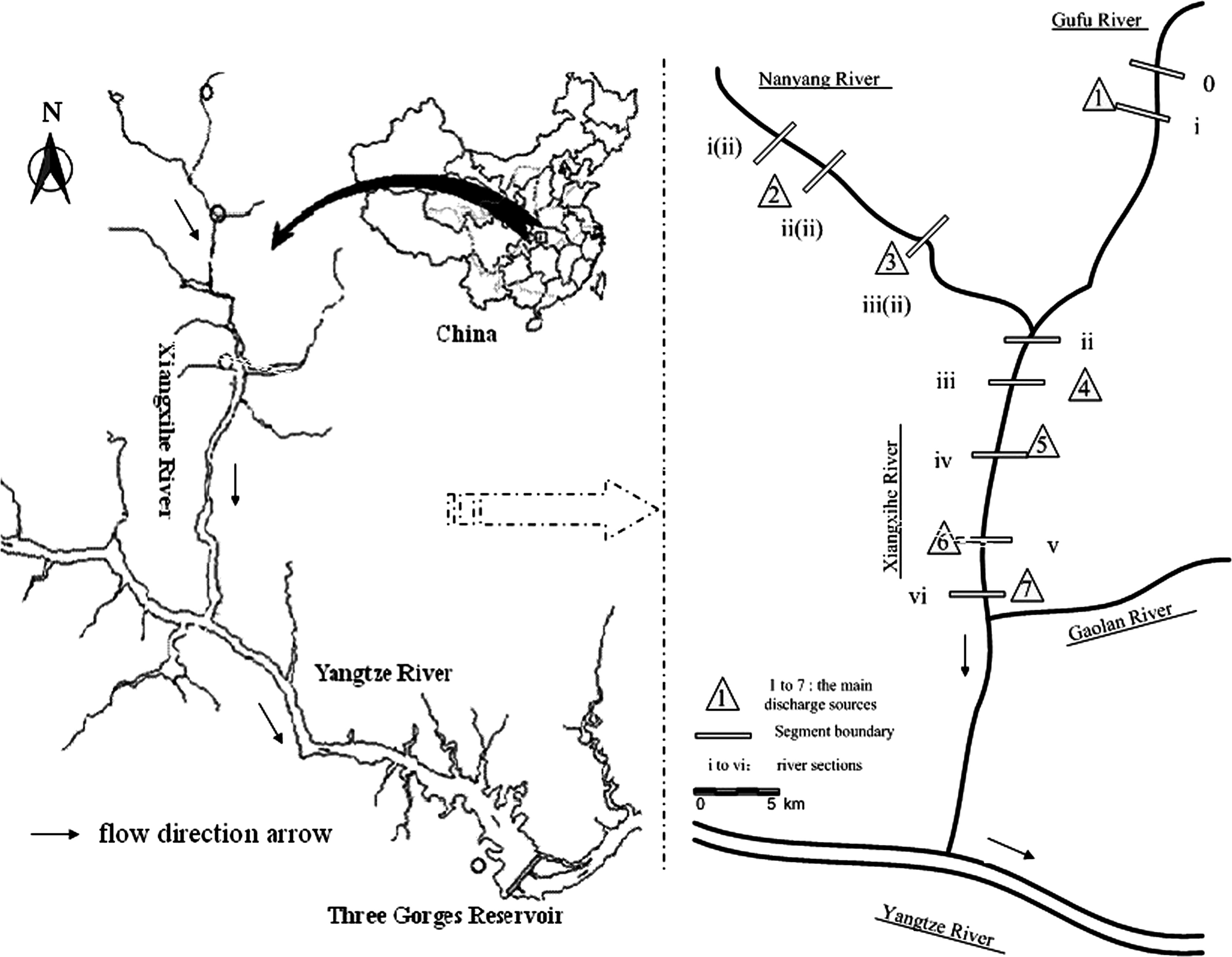
The study river system.

Xiangxihe River Basin is abundant in phosphorus resources. As one of the three richest phosphate ore districts of China, the amount of reserve phosphorus in this area is about 357 million tonnes (XGIN, 2010). Phosphorus-related industry is of great importance to local economy. With rapid local economic development, many township enterprises along the river appeared. Pollution discharge mainly focus on Gaoyan town along the river. For example, in Xiangshan County, an annual of 1.97 million tonnes of wastewater is sluiced directly into Xiangxihe River, which includes the waste of volatile phenol, petroleum, and chlorides. There are eight towns along Xiangxihe River in Xingshan County with an area of 2102 km². The total population of the area was 182.7 thousand in late 2007, of which 74.6 percent (i.e., 139.6 thousand) live in rural areas (Zhu et al., 2009b). Crop farming is the main occupation of the area, besides animal husbandry. There are 294.5 km² of tillable land of this area. The main crops are potato, corn, rice, orange, and tea and the main live stocks are pigs, cattle, and chickens (GWP, 2009). The water available in Xiangxihe River is needed for irrigation purpose, and due to the use of fertilizer, pesticide, and inadequate irrigation facilities, the backflow from the farmland pollutes the river. Due to imperfect of drainage facilities, living sewage is directly drained into Xiangxihe River. For example, the amount of nonpoint source pollution of domestic sewage is 8.2 million tonnes in 2007 (Zhu et al., 2009b). The pollutant discharge from animal husbandry, industrial wastewater, and domestic sewage are of main pollution in rural area. Water pollution became serious and environmental capacity has decreased because the immoderately discharge of sewage makes it difficult for the process of self-purification in the river. To protect the environment and maintain water quality, planning the waste discharge along the river is desired.

In this study, a length of 28 km river stretch (from Gufu town to Xiakou town) with a tributary (Nanyang River) is provided as a case to demonstrate the applicability of the proposed methodology. Seven main discharge sources exist along the river marked 1 to 7, which are considered as the point sources of pollutants, including Nanyang town WTP, Gufu town WTP, Gaoyang town WTP, Xiakou town WTP, Baishahe chemical plant, Liucaopo chemical plant, and Pingyikou cement mill (ERRX, 2009). Among them, the WTP can treat sewage from residences, and the industrial sources of wastewater require specialized treatment before being discharged to the stream. For a water quality management system of Xiangxihe River, the environmental agencies provide quality standards over the river system to control stream pollution. The stream standards are intended to maintain stream water quality by limiting the amount of waste that can be discharged into the stream. Therefore, conflict between wastewater discharge and water quality protection become increasingly serious. Currently, the situation of one-dimensional simulation model and point source pollution is suitable to pollution control for Xiangxihe River system. For example, this study deals with point source pollution, such as municipality and industry point source pollutions, but without nonpoint source pollution such as agriculture and surface runoff pollution. Environmental agencies have the responsibility to control point source pollutions by allocating BOD loadings of wastewater dischargers within Xiangxihe River. For the stream water, a minimum DO level is required for supporting aquatic life and maintaining aerobic condition. In further studies, additional water quality indicators such as chemical oxygen demand (COD), nitrogen, and phosphates can also be handled through developing similar methods. On the other hand, the water quality in the river was related to contaminant concentrations and flow rate of the discharged wastewater. The quality of discharged wastewater would then affect water quality of the receiving river body. To meet the environmental requirement, the raw wastewater from each pollution source must be treated with specific facilities before discharge. Moreover, the operating costs of these facilities are related to the inflow of wastewater and the level of its treatment; and a variety of uncertainties and nonlinearities exist in the water quality management models, which is important for analyzing system behaviors and providing decision supports for local decision makers. Thus, the simulation-based optimization model is considered to be suitable for calculating pollutant levels and minimizing both the system costs and environmental risks.

Data collection

Figure 2 shows the schematic diagram of the study system. The river system is discretized into six reaches, which are marked from i to vi, and water quality at each reach is affected by various sources from its upper stream. The tributary has two sewage outlets and is divided into three reaches which are marked from i(ii) to iii(ii), and as a pollution merges into the second reach of the main stream. The related water quality parameters that need to be considered are BOD and DO, rooting in town sewage plants and industrial emissions. Table 1 shows the water quality parameters in different river segments (Luo and Tan, 2000; Li, et al., 2003; Wang, 2005). The parameters required for water quality simulation are collected from history and observed data of Xiangxihe River. Uncertainties associated with BOD deoxygenation rate (k_di) and reaeration rate (k_ai) due to dynamic and fluctuating features were handled as intervals. Interval parameters, which are represented with a lower bound and a upper bound, do not provide information regarding how probable it is for the value to fall within the interval, nor which of the values is most likely to occur (Zhu et al., 2009a). The right-hand sides of optimization-model constraints (e.g., water quality standards) are also expressed as intervals due to its effectiveness in avoiding or mitigating violation of model solutions. According to the national standards for surface water quality of China (GB3838-2002), BOD level equal to 4 mg/L is defined as Class-III water (residential and fishery), and 6 mg/L as Class-IV water (industrial and recreational); DO level equal to 6 mg/L is defined as Class-III water and 5 mg/L as Class-IV water. However, as a tributary of Yangtze River, local governments had strict requirements on water quality criteria, and some other pollution loadings must be reserved for lacking consider agricultural nonpoint source pollution. In this study, two scenarios and three environmental criteria were examined. The intervals of allowable BOD and DO levels in the river system are identified as [3, 5] and [4, 6] mg/L, respectively. In scenario 1, the mainstream and tributary are both considered to be optimized; in scenario 2, tributary is not considered to be optimized. The environmental guidelines, where the associated uncertainties could be derived from human judgment or variations of regulatory requirements, can be effectively reduced and the wideness of regulatory intervals can be properly controlled. For example, if a stricter pollution control strategy is preferred (the stricter half parts of the intervals named standard 1), the allowable BOD and DO intervals of surface water quality can be decided as [3, 4] and [4, 5] mg/L, respectively. Similarly, the less strict half parts of the interval (standard 2) can be determined as [4, 5] and [5, 6] mg/L, respectively. BOD and DO levels are identified as [3, 5] and [4, 6] mg/L under scenario 1 is called basic case. According to the wastewater discharge standard of China (GB8978-1996), the BOD effluent levels equal to 30 mg/L (WTP) and 60 mg/L (industrial wastewater) are defined as Class-II standard, and 300 mg/L (industrial wastewater) as Class-III standard. Since there is no Class-III standard available for WTP, we assume it is 60 mg/L. Due to capacity restrictions of available wastewater treatment technologies, we assume that the maximum possible treatment efficiency for BOD is 95%. Table 2 presents the wastewater discharge data from various sources. The cost function of each discharge sources is listed in Table 3. The wastewater treatment cost functions are obtained indirectly from published reports and articles. Since the related data are historically based and estimated, the coefficients of these cost functions are imprecise and expressed as intervals. An IQP model can be formulated to tackle this problem, where the coefficients of these functions are expressed as intervals due to the uncertainties in the obtained information (e.g. k_q, k₁, and k₂).

Table 1.

Water Quality Parameters of Various River Segments

	Gufu River	Nanyang River (ii)			Xiangxihe River
River segments	i	i(ii)	ii(ii)	iii(ii)	ii	iii	iv	v	vi
Deoxygenation rate for BOD k_di (1/d)	[0.04, 0.046]	[0.045, 0.051]	[0.045, 0.51]	[0.035, 0.042]	[0.045, 0.051]	[0.03, 0.038]	[0.038, 0.045]	[0.042, 0.048]	[0.05, 0.055]
Reaeration rate k_ai (1/d)	[0.18, 0.3]	[0.2, 0.32]	[0.2, 0.32]	[0.15, 0.28]	[0.15, 0.28]	[0.15, 0.28]	[0.144, 0.274]	[0.138, 0.258]	[0.12, 0.25]

BOD, biological oxygen demand.

Table 2.

Wastewater Data from Various Discharge Sources

	Sources
Parameters	1 Gufu	2 Nanyang	3 Baishahe	4 Gaoyang	5 Pingyikou	6 Liucaopo	7 Xiakou
Raw BOD L_i (mg/L)	360	250	650	400	400	450	250
Raw DO O_i (mg/L)	0.7	1.1	0.8	1.2	0.6	0.9	1.3
Discharge rate Q_i (m³/s)	0.45	1.20	0.26	0.23	0.11	0.187	0.17

DO, dissolved oxygen.

Table 3.

Cost Functions of Different Segments

	Source	Quadratic cost function (RMB¥×10⁶)
1	Gufu	Q₁^{[0.7, 0.8]}([4.22, 5.78]+[34.32, 36.80]η₁²)
2	Nangyang	Q₂^{[0.7, 0.8]}([3.15, 4.28]+[31.50, 32.65]η₂²)
3	Baishahe	Q₃^{[0.7, 0.8]}([3.24, 4.86]+[28.60, 30.98]η₃²)
4	Gaoyang	Q₄^{[0.7, 0.8]}([3.50, 4.32]+[31.20, 33.82]η₄²)
5	Pingyikou	Q₅^{[0.7, 0.8]}([3.08, 4.12]+[30.28, 34.60]η₅²)
6	Liucaopo	Q₆^{[0.7, 0.8]}([2.60, 3.65]+[28.20, 30.00]η₆²)
7	Xiakou	Q₇^{[0.7, 0.8]}([3.15, 4.28]+[29.80, 33.65]η₇²)

Formulation of IQP model

Based on Equations (1 )–(4) with interval analysis, the interval matrixes and vectors for U^±, V^±, m^±, and n^± are obtained.

For the tributary: \documentclass{aastex}\usepackage{amsbsy}\usepackage{amsfonts}\usepackage{amssymb}\usepackage{bm}\usepackage{mathrsfs}\usepackage{pifont}\usepackage{stmaryrd}\usepackage{textcomp}\usepackage{portland,xspace}\usepackage{amsmath,amsxtra}\pagestyle{empty}\DeclareMathSizes{10}{9}{7}{6} \begin{document} \begin{align*} \vec{U}_2^{ \pm} = 10^{ - 3} \times \left[ \begin{matrix}6.205 & 0 & 0 \\ [ 5.618,5.683 ] & 13.265 & 0 \\ [ 5.33,5.44 ] & [ 12.586,12.697 ] & 0 \end{matrix} \right] \tag{ 18{\rm a} } \end{align*} \end{document} \documentclass{aastex}\usepackage{amsbsy}\usepackage{amsfonts}\usepackage{amssymb}\usepackage{bm}\usepackage{mathrsfs}\usepackage{pifont}\usepackage{stmaryrd}\usepackage{textcomp}\usepackage{portland,xspace}\usepackage{amsmath,amsxtra}\pagestyle{empty}\DeclareMathSizes{10}{9}{7}{6} \begin{document} \begin{align*} \\ \vec{V}_2^{ \pm} = - 10^{ - 3} \times \left[ \begin{matrix}0 & 0 & 0 \\ [ 0.37, 0.39 ] & 0 & 0 \\ [0.52, 0.53 ] & [0.52, 0.57] & 0 \end{matrix} \right] \tag{ 18{\rm b} } \end{align*} \end{document} \documentclass{aastex}\usepackage{amsbsy}\usepackage{amsfonts}\usepackage{amssymb}\usepackage{bm}\usepackage{mathrsfs}\usepackage{pifont}\usepackage{stmaryrd}\usepackage{textcomp}\usepackage{portland,xspace}\usepackage{amsmath,amsxtra}\pagestyle{empty}\DeclareMathSizes{10}{9}{7}{6} \begin{document} \begin{align*} \vec{m}_2^{ \pm} = ( [ 2.897 , 2.908 ] \ [ 2.623 , 2.664 ] \ [ 2.489 , 2.550 ] ) ^T \tag{ 18{\rm c} } \end{align*} \end{document} \documentclass{aastex}\usepackage{amsbsy}\usepackage{amsfonts}\usepackage{amssymb}\usepackage{bm}\usepackage{mathrsfs}\usepackage{pifont}\usepackage{stmaryrd}\usepackage{textcomp}\usepackage{portland,xspace}\usepackage{amsmath,amsxtra}\pagestyle{empty}\DeclareMathSizes{10}{9}{7}{6} \begin{document} \begin{align*} \vec{n}_2^{ \pm} = ( [ 8.095 , 8.201 ] \ [ 8.353 , 8.650 ] \ [ 8.531 , 8.936 ] ) ^T \tag{ 18{\rm d} } \end{align*} \end{document} \documentclass{aastex}\usepackage{amsbsy}\usepackage{amsfonts}\usepackage{amssymb}\usepackage{bm}\usepackage{mathrsfs}\usepackage{pifont}\usepackage{stmaryrd}\usepackage{textcomp}\usepackage{portland,xspace}\usepackage{amsmath,amsxtra}\pagestyle{empty}\DeclareMathSizes{10}{9}{7}{6} \begin{document} \begin{align*} L_{2_j} = \mathop\sum_{i = 1}^3 [ U_{2ji}^{ \pm}L_{2i} ( 1 - \eta_i^{ \pm} ) ] + m_{2j}^{ \pm} \quad j = 1 , 2 , 3 \tag{ 18{\rm e} } \end{align*} \end{document}

For the mainstream:

where \documentclass{aastex}\usepackage{amsbsy}\usepackage{amsfonts}\usepackage{amssymb}\usepackage{bm}\usepackage{mathrsfs}\usepackage{pifont}\usepackage{stmaryrd}\usepackage{textcomp}\usepackage{portland, xspace}\usepackage{amsmath, amsxtra}\pagestyle{empty}\DeclareMathSizes {10} {9} {7} {6} \begin{document} $$\vec{L}_2 = ( 250 \ 650 \ 0 ) ^T$$ \end{document} ; L₂₃ is BOD concentration at the last section of tributary that treated as a source of pollution. \documentclass{aastex}\usepackage{amsbsy}\usepackage{amsfonts}\usepackage{amssymb}\usepackage{bm}\usepackage{mathrsfs}\usepackage{pifont}\usepackage{stmaryrd}\usepackage{textcomp}\usepackage{portland,xspace}\usepackage{amsmath,amsxtra}\pagestyle{empty}\DeclareMathSizes{10}{9}{7}{6} \begin{document} \begin{align*} \vec{U}^{\pm} &= 10^{-3} \times \left[\begin{matrix}22.632 &0 &0 &0 &0 &0 \\ [9.834,10.006] &496.416 &0 &0 &0 &0 \\ [9.378,9.626] \ &[473.429,477.594] \ &5.792 &0 &0 &0 \\ [8.473,8.832] \ &[427.715,438.159] \ &[5.232,5.313] &2.762 &0 &0 \\ [7.425,7.864] \ &[374.824,390.136] \ &[4.585,4.731] \ &[2.421,2.459] &4.674 &0 \\ [6.938,7.39] \ &[350.22,366.642] \ &[4.284,4.446] \ &[2.262,2.311] \ &[4.367,4.392] \ &4.231\end{matrix}\right] &(19{\rm a}) \\ \vec{V}^{\pm} &= -10^{-3} \times \left[\begin{matrix}0 &0 &0 &0 &0 &0 \\ [1.06,1.12] \ &0 &0 &0 &0 &0\\ [1.12,1.24] \ &[14.7,17.3] &0 &0 &0 &0 \\ [1.27,1.56] \ &[42.66,43.29] \ &[0.4,0.41] &0 &0 &0 \\ [1.35,1.85] \ &[58.01,68.25] \ &[0.65,0.74] &0.24 &0 &0 \\ [1.41,2.02] \ &[63.21,79.53] \ &[0.73,0.89] \ &[0.31,0.34] \ &[0.24,0.25] &0\end{matrix}\right] &(19{\rm b}) \\ \vec{m}^{\pm} &= ([2.855,2.865] \ [1.241,1.267] \ [1.183,1.219] \ [1.069,1.118] \ [0.937,0.995] \ [0.875,0.936])^T &(19{\rm c}) \\ \vec{n}^{\pm} &= \{[7.964,8.076] \ [8.231,8.658] \ [8.419,8.924] \ [8.742,9.303] \ [8.991,9.516] \ [9.037,9.553]\}^T &(19{\rm d}) \\ \vec{L} &= (360 \ L_{23}^{\pm} \ 400 \ 400 \ 450 \ 250)^T &(19{\rm e}) \end{align*} \end{document}

The objective of the IQP model can be formulated as: \documentclass{aastex}\usepackage{amsbsy}\usepackage{amsfonts}\usepackage{amssymb}\usepackage{bm}\usepackage{mathrsfs}\usepackage{pifont}\usepackage{stmaryrd}\usepackage{textcomp}\usepackage{portland,xspace}\usepackage{amsmath,amsxtra}\pagestyle{empty}\DeclareMathSizes{10}{9}{7}{6} \begin{document} \begin{align*} \begin{split} \min f^{ \pm} = { \rm Q}_1^{ [ 0.7 , \ 0.8 ] } ( [ 422 , 578 ] + [ 3432 , 3680 ] \eta_1^2 ) \\\quad+ { \rm Q}_2^{ [ 0.7 , \ 0.8 ] } ( [ 315 , 428 ] + [ 3150 , 3265 ] \eta_2^2 ) \\ \quad+ { \rm Q}_3^{ [ 0.7 , \ 0.8 ] } ( [ 324 , 486 ] + [ 2860 , 3098 ] \eta_3^2 ) \\\quad+ { \rm Q}_4^{ [ 0.7 , \ 0.8 ] } ( [ 350 , 432 ] + [ 3120 , 3382 ] \eta_4^2 ) \\ \quad+ { \rm Q}_5^{ [ 0.7 , \ 0.8 ] } ( [ 308 , 412 ] + [ 3028 , 3460 ] \eta_5^2 ) \\\quad+ { \rm Q}_6^{ [ 0.7 , \ 0.8 ] } ( [ 260 , 365 ] + [ 2820 , 3000 ] \eta_6^2 ) \\ \quad+ { \rm Q}_7^{ [ 0.7 , \ 0.8 ] } ( [ 315 , 428 ] + [ 2980 , 3365 ] \eta_7^2 ) \end{split} \tag{20}\end{align*} \end{document}

Based on water quality simulation models with interval analysis, the IQP model can be formulated as Equation (15), and the detailed solution process for the proposed model can be obtained from section 2.3.

Results and Discussion

Figure 3 presents the results obtained from IQP model. Solutions for the objective function value and decision variables are interval numbers. Given different water quality requirements and BOD discharge concentrations, the efficiency in WTP would vary between their relevant solution intervals. Planning for the lower bound of the system cost (e.g., RMB¥ 40.87×10⁶) leads to a lower wastewater treatment efficiency ( \documentclass{aastex}\usepackage{amsbsy}\usepackage{amsfonts}\usepackage{amssymb}\usepackage{bm}\usepackage{mathrsfs}\usepackage{pifont}\usepackage{stmaryrd}\usepackage{textcomp}\usepackage{portland, xspace}\usepackage{amsmath, amsxtra}\pagestyle{empty}\DeclareMathSizes {10} {9} {7} {6} \begin{document} $$\eta_i^ -$$ \end{document} ); decision at the upper-bound system cost (i.e., RMB¥ 77.99×10⁶) is associated with a high wastewater treatment efficiency ( \documentclass{aastex}\usepackage{amsbsy}\usepackage{amsfonts}\usepackage{amssymb}\usepackage{bm}\usepackage{mathrsfs}\usepackage{pifont}\usepackage{stmaryrd}\usepackage{textcomp}\usepackage{portland, xspace}\usepackage{amsmath, amsxtra}\pagestyle{empty}\DeclareMathSizes {10} {9} {7} {6} \begin{document} $$\eta_i^ +$$ \end{document} ). Thus, when different wastewater treatment settings are selected from their interval solutions, the relevant system cost will vary within intervals correspondingly. The study problem can also be solved by a deterministic programming method under mid value case, through simplifying the interval value into mid value (i.e., V_mid=[V⁻+V⁺]/2) under scenario 1. Then, the IQP model can be converted into a mid value QP problem. The results obtained through the mid value QP model for wastewater treatment efficiency of different discharge sources compared with the IQP model optimization results are shown in Fig. 3. The system cost according to mid value QP model is RMB¥ 55.46×10⁶, which is a certain appropriate value between the lower and upper bounds of the objective function. It appears that required treatment efficiencies of the municipalities (Gufu WTP [83.3%, 97.0%], Nanyang [76.0%, 94.6%], and Xiakou [76.0%, 88.0%]) are more stringent than those of industries (Pingyikou [38.6%, 85.0%] and Liucaopo [53.9%, 86.7%]). Obviously, sources with low BOD discharge standard for municipalities (i.e., [30, 60] mg/L) need stricter treatment requirements to meet water quality standard.

FIG. 3.

Model solutions of basic and midvalue case.

In many cases, combinations of different treatment processes could be used to meet required standards, since each type of treatment has a certain efficiency range for different quality parameters. Tertiary treatment facility would have to be used to reach high pollutant removal efficiencies. In general, a secondary treatment would be sufficient for most of the discharge sources under an optimistic consideration. However, when environmental protection is of severe concern by the local government, all discharge sources would require the tertiary treatment. The solutions at the lower bounds represent a situation when the decision makers are optimistic about the water quality and wastewater discharges under this studying system. Disadvantageous condition corresponds to a situation when the decision makers are optimistic about the system that could not reach the water quality criteria. In such a case, lower treatment requirements are desired. If the plan aims toward a lower treatment requirement, the risk of violating the relevant water quality criteria would increase under disadvantageous conditions. Table 4 presents several alternatives obtained by adjusting decision-variable values within their solution intervals. Alternative 1 is associated with upper-bound levels of wastewater treatment efficiencies, and could result in a high system cost, meanwhile, lower risk of violating the water quality standards. Conversely, when the wastewater treatment efficiencies reach their lower-bound levels, there would be a lower system cost, but an increased risk of unsafe water quality (i.e., alternative 4). When the decision makers have a moderate attitude toward system cost and environmental risk, alternatives 2 and 3 would become more realistic. These alternatives represent a compromise between wastewater treatment cost and environmental requirements. In general, the provided alternatives represent multiple decision options with various economic and environmental considerations.

Table 4.

Decision Alternatives Generated from the Interval Values

	Wastewater treatment efficiencies
Alternative	1 Gufu	2 Nanyang	3 Baishahe	4 Gaoyang	5 Pingyikou	6 Liucaopo	7 Xiakou	System cost (RMB¥10⁶)
1	−	−	−	−	−	−	−	[40.87, 53.00]
2	−	+	+	−	−	−	−	[46.19, 59.66]
3	+	−	−	+	+	+	+	[55.27, 71.32]
4	+	+	+	+	+	+	+	[60.58, 77.99]

+, upper-bound value; −, lower-bound value.

Figures 4 and 5 present the optimization solutions under standards 1 and 2, respectively, with the mainstream and tributary are both considered to be optimized. The basic solution intervals (e.g., Gufu [83.3%, 97.0%]) to the IQP model are divided into two different parts (i.e., Gufu [85.9%, 97.0%] and [83.3%, 91.7%]). The interval results under scenario 1 with two different standards (BOD [3, 4] and [4, 5] mg/L) indicate that the upper parts of intervals are obtained under strict environmental criteria, and the lower parts are from the looser environmental criteria. In practical applications, allowable levels of environmental violations could be decided based on discussions among stakeholders, and the decision variables could be adjusted continuously within their solution intervals under specific environmental standards. Different optimal values of lower and upper bound of wastewater treatment efficiencies will generate different cost effective water quality management schemes, but the interval parameter programming (IPP) techniques for reducing the right hand side uncertainties will remain same.

FIG. 4.

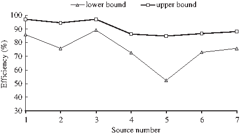
Solutions under standard 1 (scenario 1).

FIG. 5.

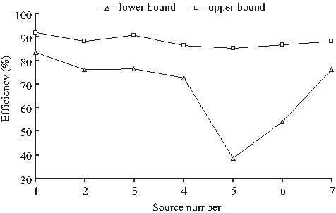
Solutions under standard 2 (scenario 1).

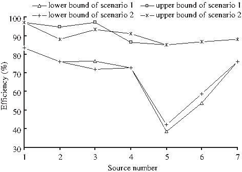
Figure 6 presents the interval solutions from the IQP model for decisions under two different scenarios. The width of the interval efficiency is high in scenario 1, implying a higher system uncertainty compared to scenario 2. For example, the wastewater treatment efficiencies for the main stream in scenarios 1 and 2 are [38.6, 85]%, [53.9, 86.7]%, [76.0, 88.0]% and [42, 85]%, [58.7, 86.7]%, [76.0, 88.0]%, respectively. The results demonstrate that the optimization model can effectively generate inexact solutions corresponding to the two different scenarios, which are decided by decision makers according to environmental requirements and local economic development. The decision alternatives can be obtained by adjusting different combinations of the decision variables within their solution intervals. With this two different scenarios and different environmental standards, the system cost would be different and interval values according to the IQP model.

FIG. 6.

Solutions under scenarios 1 and 2.

Figure 7 presents the system cost of different environmental standards (the allowable BOD of surface water quality, that is, [3, 5], [3, 4], and [4, 5] mg/L) under scenarios 1 and 2. Scenario 1 represents a situation when the manager is strict with the wastewater discharge along the river, and thus desires to optimistically environmental conditions. The results indicate that the system costs are RMB¥ [40.87, 77.99]×10⁶ under standard 1, RMB¥ [46.28, 77.99]×10⁶ under standard 2, and RMB¥ [40.87, 73.57]×10⁶ under basic case standard. In comparison, scenario 2 is a conservative policy corresponding to low treatment efficiencies and wastewater treatment cost. This will lead to a high risk of environmental pollution of the river system. The above inexact solutions, according to different optimization scenarios and environmental requirements, can be further interpreted to generate decision alternatives.

FIG. 7.

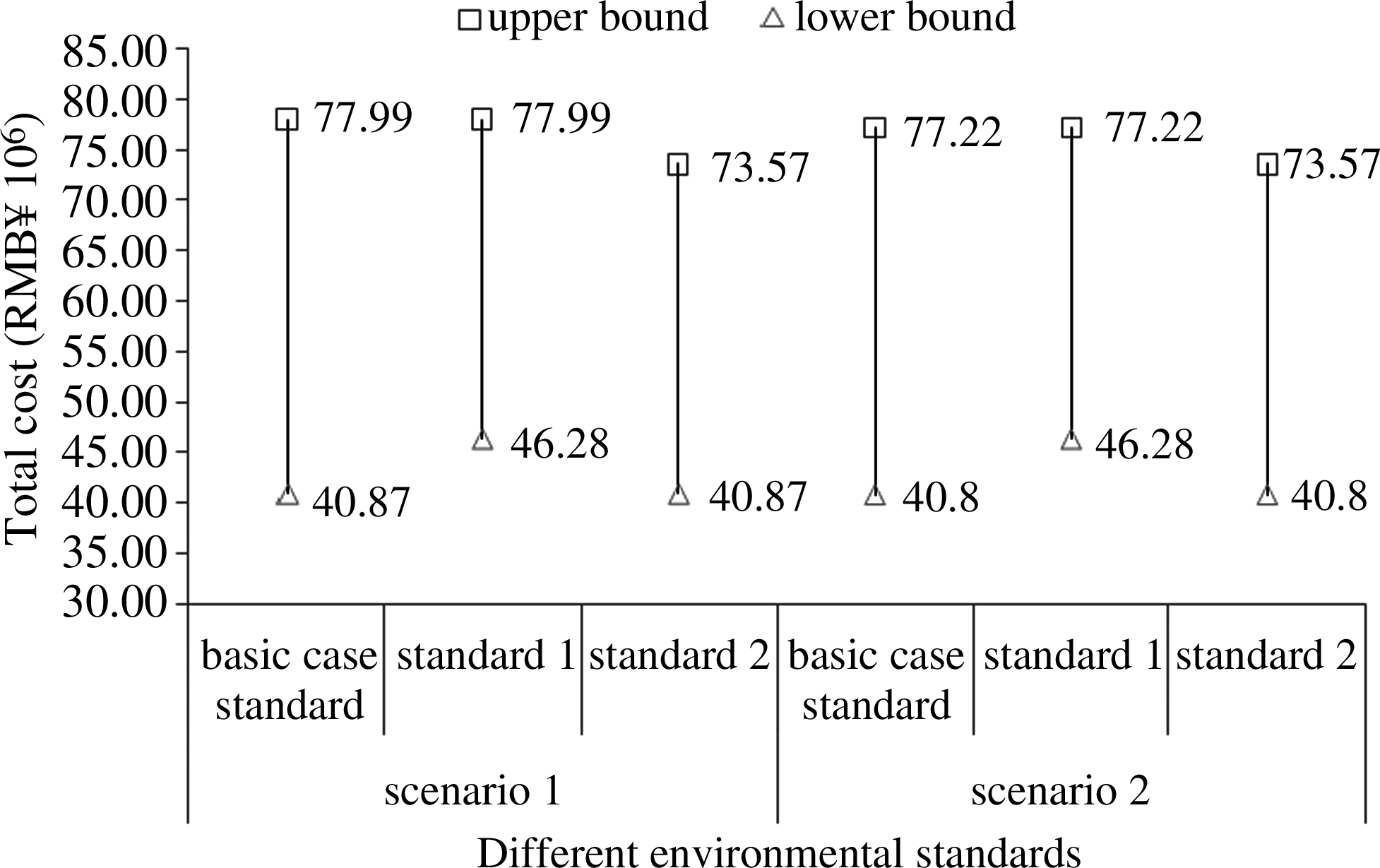
System cost of different environmental standards under scenarios 1 and 2.

Figure 8 describes the stream water quality under different policy scenarios and environmental standards. BOD levels at each river section could be calculated through the water quality simulation model [Eq. (3a)]. Scenario 1 is a conservation policy corresponding to high wastewater treatment efficiencies and high system cost. This lead to a plan with lower pollutant levels, where BOD concentrations at each river section could meet local environmental requirement. Scenario 2 is a situation when the local decision makers are optimistic regarding the environmental conditions, and thus desire to fuel local industry expansion. Under this policy scenario, the water quality of the tributary would be polluted. The results shown in Fig. 8 indicate that the tributary contribute more pollution to the river.

FIG. 8.

Biological oxygen demand (BOD) concentration in stream of different sections under scenarios 1 and 2.

For a tributary, the last section of the river segments could be introduced to the main river as a source of wastewater discharge. The wastewater of discharges of the tributary need enhanced treatment to satisfy local environmental requirement. The wastewater treatment efficiency of five discharge sources on mainstream and BOD level at the tributary that treated as a source of pollution would calculate from the optimization model of this study. Under these two different policy scenarios and environmental standards, the BOD level at each segment of mainstream considered as a constraint according to the model would meet the needs of local environmental policy, whereas the BOD level at each segment of tributary may be not. The BOD levels of each tributary segment are obtained when decision makers think that economic development is the first priority. The BOD levels of Nanyang River (i.e., [3.27, 5.38], [3.10, 3.42] mg/L) are greater than the local environmental criteria. The interval-parameter programming can incorporate uncertain information within its modeling framework and provide solutions presented as intervals to help decision makers analyze the tradeoffs between system cost and system-failure risk. The allowable levels of environmental violations could be decided based on discussions among stakeholders according to specific system conditions (system cost, system-failure risk, and river pollution situations under two scenarios and three criteria in this study). This would allow local decision makers to incorporate more socioeconomic conditions within decision framework, if required for the decision.

Conclusions

In this article, an IQP model has been developed for stream water quality management, which is based on approaches of IPP and quadratic programming (QP). The IQP can deal with uncertainties associated with water quality parameters, cost functions, and environmental guidelines existed as interval parameters and objective function expressed as nonlinearities. In its solution process, the IQP model is transformed into two deterministic submodels, which correspond to the lower and upper bounds of the objective function. Interval solutions can then be generated by solving the two submodels sequentially. The proposed IQP method has been applied to water quality management of Xiangxihe River, China. The water simulation system proposed in this study is suitable for one-dimensional stream water quality management systems, with BOD and DO levels being the main water quality indicators. The water quality simulation equations are derived from the river system assuming a steady-state flow regime in each of its divided segments. By this water quality simulation, it can provide an effective linkage between wastewater treatment cost and water quality goals. Decision alternatives can be obtained by adjusting different combinations of the decision variables within their solution intervals. The results indicate that IQP is applicable to problems associated with nonlinearities and uncertainties. A cost-effective water quality management scheme is generated, where wastewater discharge is recommended. The model results will be useful for optimal policy-making concerning local economic development and environmental requirement. The research work is advantageous in the following aspects: (1) a multisegment water quality model was developed to generate water quality transformation matrices and vectors, which could be embedded directly into a water quality management model; (2) the mainstream with n sections, and its tributary with m(i) sections treated as a source of pollution will be introduced into the matrix equation to calculate water quality level of the mainstream; and (3) uncertainties associated with water quality parameters could be projected to optimization models through interval analysis and the nonlinearity problem associated with the objective function of wastewater treatment could be expressed as QP.

Although reasonable solutions have been obtained considering local environmental requirements and policymakers' choices between environment and economy, regarding Xiangxihe River Basin, this may have limitations because model parameters are unacceptable and real case is immensely complex, and hard to simplify. Moreover, IQP has difficulties in addressing uncertainties presented in terms of probabilistic and/or possibilistic distributions. It could also be coupled with other optimization methodologies (e.g., fuzzy programming) to handle more uncertainties in water quality management problems. In this study, the major pollution source is point source pollution. Since agricultural, animal husbandry, and surface runoff are also significant pollution of river water quality, it is desired to tackle this nonpoint source pollution. To protect the river from excessive inputs of nutrients and pollutants, the wastewater discharged from phosphorus-related industry must be treated. In future studies, additional water quality indicators such as COD, nitrogen, and phosphates can also be handled through developing similar methods. Therefore, further studies are desired to mitigate these limitations.

Footnotes

Acknowledgments

This research was supported by the Major Science and Technology Program for Water Pollution Control and Treatment (2009ZX07104-004). The authors are grateful to the editors and the anonymous reviewers for their insightful comments and suggestions.

Author Disclosure Statement

No competing financial interests exist.

Appendix

The basic biological oxygen demand–dissolved oxygen (BOD-DO) relations can be written as: \documentclass{aastex}\usepackage{amsbsy}\usepackage{amsfonts}\usepackage{amssymb}\usepackage{bm}\usepackage{mathrsfs}\usepackage{pifont}\usepackage{stmaryrd}\usepackage{textcomp}\usepackage{portland,xspace}\usepackage{amsmath,amsxtra}\pagestyle{empty}\DeclareMathSizes{10}{9}{7}{6} \begin{document} \begin{align*} \frac { dL } { dt } = - k_d L \tag{ \rm {A-1a} } \end{align*} \end{document} \documentclass{aastex}\usepackage{amsbsy}\usepackage{amsfonts}\usepackage{amssymb}\usepackage{bm}\usepackage{mathrsfs}\usepackage{pifont}\usepackage{stmaryrd}\usepackage{textcomp}\usepackage{portland,xspace}\usepackage{amsmath,amsxtra}\pagestyle{empty}\DeclareMathSizes{10}{9}{7}{6} \begin{document} \begin{align*} \frac { dO } { dt } = k_d L - k_a ( O_s - O ) \tag{ \rm {A-1b} } \end{align*} \end{document}

where L is the ultimate BOD concentration, O is the DO concentration, O_s is the saturated DO concentration, t is the mean flow time, k_a is the first-order reaeration rate constant, and k_d is the first-order deoxygenation rate constant.

The solution of above equations is: \documentclass{aastex}\usepackage{amsbsy}\usepackage{amsfonts}\usepackage{amssymb}\usepackage{bm}\usepackage{mathrsfs}\usepackage{pifont}\usepackage{stmaryrd}\usepackage{textcomp}\usepackage{portland,xspace}\usepackage{amsmath,amsxtra}\pagestyle{empty}\DeclareMathSizes{10}{9}{7}{6} \begin{document} \begin{align*} L = L_0 e^{ - k_d x / u} \tag{ \rm {A-2a}} \end{align*} \end{document} \documentclass{aastex}\usepackage{amsbsy}\usepackage{amsfonts}\usepackage{amssymb}\usepackage{bm}\usepackage{mathrsfs}\usepackage{pifont}\usepackage{stmaryrd}\usepackage{textcomp}\usepackage{portland,xspace}\usepackage{amsmath,amsxtra}\pagestyle{empty}\DeclareMathSizes{10}{9}{7}{6} \begin{document} \begin{align*} O = O_s - \frac { k_d L_0 } { k_a - k_d } \Big[ e^ { - k_d x / u } - e^ { - k_a x / u } \Big] - ( O_s - O_0 ) e^ { - k_a x / u } \tag{ \rm {A-2b} } \end{align*} \end{document}

where L₀ and O₀ are BOD and DO concentrations at the starting point of the river system, respectively. μ is the average stream flow rate, and x is the flow distance along the x axis.

Segmenting a stream into multiple reaches is necessary since a number of wastewater discharge outlets scatter along the river, with temporal and spatial variations of their loadings. According to Appendix Fig. A1, the equations of mass balance, flow continuity, flow rate, and BOD equilibrium of a river system can be written as follows: \documentclass{aastex}\usepackage{amsbsy}\usepackage{amsfonts}\usepackage{amssymb}\usepackage{bm}\usepackage{mathrsfs}\usepackage{pifont}\usepackage{stmaryrd}\usepackage{textcomp}\usepackage{portland,xspace}\usepackage{amsmath,amsxtra}\pagestyle{empty}\DeclareMathSizes{10}{9}{7}{6} \begin{document} \begin{align*} Q_{2i} = Q_{1i} - Q_{3i} + Q_i \tag{\rm{A-3a} } \end{align*} \end{document} \documentclass{aastex}\usepackage{amsbsy}\usepackage{amsfonts}\usepackage{amssymb}\usepackage{bm}\usepackage{mathrsfs}\usepackage{pifont}\usepackage{stmaryrd}\usepackage{textcomp}\usepackage{portland,xspace}\usepackage{amsmath,amsxtra}\pagestyle{empty}\DeclareMathSizes{10}{9}{7}{6} \begin{document} \begin{align*} Q_{1i} = Q_{2 , i - 1} \tag{\rm{A-3b} } \end{align*} \end{document} \documentclass{aastex}\usepackage{amsbsy}\usepackage{amsfonts}\usepackage{amssymb}\usepackage{bm}\usepackage{mathrsfs}\usepackage{pifont}\usepackage{stmaryrd}\usepackage{textcomp}\usepackage{portland,xspace}\usepackage{amsmath,amsxtra}\pagestyle{empty}\DeclareMathSizes{10}{9}{7}{6} \begin{document} \begin{align*} L_{2i}Q_{2i} = L_{1i} ( Q_{1i} - Q_{3i} ) + L_iQ_i \tag{ \rm{A-3c} } \end{align*} \end{document} \documentclass{aastex}\usepackage{amsbsy}\usepackage{amsfonts}\usepackage{amssymb}\usepackage{bm}\usepackage{mathrsfs}\usepackage{pifont}\usepackage{stmaryrd}\usepackage{textcomp}\usepackage{portland,xspace}\usepackage{amsmath,amsxtra}\pagestyle{empty}\DeclareMathSizes{10}{9}{7}{6} \begin{document} \begin{align*} O_{2i}Q_{2i} = O_{1i} ( Q_{1i} - Q_{3i} ) + O_iQ_i \tag{\rm{A-3d} } \end{align*} \end{document}

From Equation (A-2a), the BOD degradation process from section i−1 to i can be written as: \documentclass{aastex}\usepackage{amsbsy}\usepackage{amsfonts}\usepackage{amssymb}\usepackage{bm}\usepackage{mathrsfs}\usepackage{pifont}\usepackage{stmaryrd}\usepackage{textcomp}\usepackage{portland,xspace}\usepackage{amsmath,amsxtra}\pagestyle{empty}\DeclareMathSizes{10}{9}{7}{6} \begin{document} \begin{align*} L_{1i} = \alpha_{i - 1}L_{2 , i - 1} \tag{\rm{A-4}} \end{align*} \end{document}

From Equations (A-3c) and (A-4), we have: \documentclass{aastex}\usepackage{amsbsy}\usepackage{amsfonts}\usepackage{amssymb}\usepackage{bm}\usepackage{mathrsfs}\usepackage{pifont}\usepackage{stmaryrd}\usepackage{textcomp}\usepackage{portland,xspace}\usepackage{amsmath,amsxtra}\pagestyle{empty}\DeclareMathSizes{10}{9}{7}{6} \begin{document} \begin{align*} L_{2i} = \alpha_{i - 1}L_{2 , i - 1} + b_i L_i \tag{\rm{A-5}} \end{align*} \end{document}

A matrix expression can thus be used to replace Equation (A-5): \documentclass{aastex}\usepackage{amsbsy}\usepackage{amsfonts}\usepackage{amssymb}\usepackage{bm}\usepackage{mathrsfs}\usepackage{pifont}\usepackage{stmaryrd}\usepackage{textcomp}\usepackage{portland,xspace}\usepackage{amsmath,amsxtra}\pagestyle{empty}\DeclareMathSizes{10}{9}{7}{6} \begin{document} \begin{align*} A \vec{L}_2 = B \vec{L} + \vec{g} \tag{\rm{A-6}} \end{align*} \end{document}

where A and B are n×n matrixes, and \documentclass{aastex}\usepackage{amsbsy}\usepackage{amsfonts}\usepackage{amssymb}\usepackage{bm}\usepackage{mathrsfs}\usepackage{pifont}\usepackage{stmaryrd}\usepackage{textcomp}\usepackage{portland, xspace}\usepackage{amsmath, amsxtra}\pagestyle{empty}\DeclareMathSizes {10} {9} {7} {6} \begin{document} $$\vec{g}$$ \end{document} is an n-dimensional vector. \documentclass{aastex}\usepackage{amsbsy}\usepackage{amsfonts}\usepackage{amssymb}\usepackage{bm}\usepackage{mathrsfs}\usepackage{pifont}\usepackage{stmaryrd}\usepackage{textcomp}\usepackage{portland,xspace}\usepackage{amsmath,amsxtra}\pagestyle{empty}\DeclareMathSizes{10}{9}{7}{6} \begin{document} \begin{align*} A = \left \{ \begin{matrix}1 & 0 & \cdots & \cdots & \cdots & 0 \\ - a_1 & 1 & 0 & & & \vdots \\ 0 & \ddots & 1 & \ddots & &\vdots\\ \vdots & 0 &- a_{i - 1} & \ddots & 0 & \vdots \\ \vdots & & \ddots & \ddots & 1 & 0 \\ 0 & \cdots & \cdots & 0 & - a_{n - 1} & 1\end{matrix} \right \} , \end{align*} \end{document} \documentclass{aastex}\usepackage{amsbsy}\usepackage{amsfonts}\usepackage{amssymb}\usepackage{bm}\usepackage{mathrsfs}\usepackage{pifont}\usepackage{stmaryrd}\usepackage{textcomp}\usepackage{portland,xspace}\usepackage{amsmath,amsxtra}\pagestyle{empty}\DeclareMathSizes{10}{9}{7}{6} \begin{document} \begin{align*} B = \left \{ \begin{matrix}b_1 & 0 & \cdots & \cdots & \cdots & 0 \\ 0 & b_2 & 0 & & & \vdots \\ 0 & \ddots & 1 & \ddots & & \vdots \\ \vdots & & & \ddots & 0 & \vdots \\ \vdots & & \ddots & \ddots & 1 & 0 \\ 0 & \cdots & \cdots & \cdots & 0 &1\end{matrix} \right \} \end{align*} \end{document} \documentclass{aastex}\usepackage{amsbsy}\usepackage{amsfonts}\usepackage{amssymb}\usepackage{bm}\usepackage{mathrsfs}\usepackage{pifont}\usepackage{stmaryrd}\usepackage{textcomp}\usepackage{portland,xspace}\usepackage{amsmath,amsxtra}\pagestyle{empty}\DeclareMathSizes{10}{9}{7}{6} \begin{document} \begin{align*} \vec{L}_2 = ( L_{21} , \ L_{22} , \ \cdots , \ L_{2n} ) ^T , \ \vec{L} = ( L_1 , \ L_2 , \ \cdots , \ L_n ) ^T \end{align*} \end{document} \documentclass{aastex}\usepackage{amsbsy}\usepackage{amsfonts}\usepackage{amssymb}\usepackage{bm}\usepackage{mathrsfs}\usepackage{pifont}\usepackage{stmaryrd}\usepackage{textcomp}\usepackage{portland,xspace}\usepackage{amsmath,amsxtra}\pagestyle{empty}\DeclareMathSizes{10}{9}{7}{6} \begin{document} \begin{align*} \vec{g} = ( g_1 , g_2 , \cdots , g_n ) ^T , {\rm and}\ g_i = \begin{cases} \quad a_0L_{20} , i = 1 \\ 0 , i = 2 , 3 , \cdots , n\end{cases} \end{align*} \end{document}

Thus, we have: \documentclass{aastex}\usepackage{amsbsy}\usepackage{amsfonts}\usepackage{amssymb}\usepackage{bm}\usepackage{mathrsfs}\usepackage{pifont}\usepackage{stmaryrd}\usepackage{textcomp}\usepackage{portland,xspace}\usepackage{amsmath,amsxtra}\pagestyle{empty}\DeclareMathSizes{10}{9}{7}{6} \begin{document} \begin{align*} \vec{L}_2 = A^{ - 1}B \vec{L} + A^{ - 1} \vec{L} \tag{\rm{A-7}} \end{align*} \end{document}

According to Equation (A-2c), the DO level can be given by: \documentclass{aastex}\usepackage{amsbsy}\usepackage{amsfonts}\usepackage{amssymb}\usepackage{bm}\usepackage{mathrsfs}\usepackage{pifont}\usepackage{stmaryrd}\usepackage{textcomp}\usepackage{portland,xspace}\usepackage{amsmath,amsxtra}\pagestyle{empty}\DeclareMathSizes{10}{9}{7}{6} \begin{document} \begin{align*} O_{1i} = O_{2i}e^{ - k_{a , i - 1}t_{i - 1}} - {k_{d , i - 1}L_{2 , i - 1} \over k_{a , i - 1} - k_{d , i - 1}} ( e^{ - k_{d , i - 1}t_{i - 1}} - e^{ - k_{a , i - 1}t_{i - 1}} ) + O_s ( 1 - e^{ - k_{a , i - 1}t_{i - 1}} ) \tag{ \rm{A-9} } \end{align*} \end{document}

Then, Equation (A-3d) becomes: \documentclass{aastex}\usepackage{amsbsy}\usepackage{amsfonts}\usepackage{amssymb}\usepackage{bm}\usepackage{mathrsfs}\usepackage{pifont}\usepackage{stmaryrd}\usepackage{textcomp}\usepackage{portland,xspace}\usepackage{amsmath,amsxtra}\pagestyle{empty}\DeclareMathSizes{10}{9}{7}{6} \begin{document} \begin{align*} O_ { 2i } = \frac { Q_ { 1i } - Q_ { 3i } } { Q_ { 2i } } ( Q_ { 2 , i - 1 } \gamma_ { i - 1 } - L_ { 2 , i - 1 } \beta_ { i - 1 } ) + \frac { Q_i } { Q_ { 2i } } O_i \tag { \rm {A-10} } \end{align*} \end{document}

Defining \documentclass{aastex}\usepackage{amsbsy}\usepackage{amsfonts}\usepackage{amssymb}\usepackage{bm}\usepackage{mathrsfs}\usepackage{pifont}\usepackage{stmaryrd}\usepackage{textcomp}\usepackage{portland, xspace}\usepackage{amsmath, amsxtra}\pagestyle{empty}\DeclareMathSizes {10} {9} {7} {6} \begin{document} $$c_ { i - 1 } ^ { \prime } = \displaystyle { \frac { Q_ { 1i } - Q_ { 3i } } { Q_ { 2i } } \gamma_ { i - 1 } } , \ d_ { i - 1 } = \frac { Q_ { 1i } - Q_ { 3i } } { Q_ { 2i } } \beta_ { i - 1 } $$ \end{document} , and \documentclass{aastex}\usepackage{amsbsy}\usepackage{amsfonts}\usepackage{amssymb}\usepackage{bm}\usepackage{mathrsfs}\usepackage{pifont}\usepackage{stmaryrd}\usepackage{textcomp}\usepackage{portland, xspace}\usepackage{amsmath, amsxtra}\pagestyle{empty}\DeclareMathSizes {10} {9} {7} {6} \begin{document} $$f_ { i - 1 } = \displaystyle { \frac { Q_ { 1i } - Q_ { 3i } } { Q_ { 2i } } \delta_ { i - 1 } } $$ \end{document}

Then, we have: \documentclass{aastex}\usepackage{amsbsy}\usepackage{amsfonts}\usepackage{amssymb}\usepackage{bm}\usepackage{mathrsfs}\usepackage{pifont}\usepackage{stmaryrd}\usepackage{textcomp}\usepackage{portland,xspace}\usepackage{amsmath,amsxtra}\pagestyle{empty}\DeclareMathSizes{10}{9}{7}{6} \begin{document} \begin{align*} O_ { 2i } = \frac { Q_ { 1i } - Q_ { 3i } } { Q_ { 2i } } ( Q_ { 2 , i - 1 } \gamma_ { i - 1 } - L_ { 2 , i - 1 } \beta_ { i - 1 } ) + \frac { Q_i } { Q_ { 2i } } O_i \tag{ \rm {A-11a} } \end{align*} \end{document} \documentclass{aastex}\usepackage{amsbsy}\usepackage{amsfonts}\usepackage{amssymb}\usepackage{bm}\usepackage{mathrsfs}\usepackage{pifont}\usepackage{stmaryrd}\usepackage{textcomp}\usepackage{portland,xspace}\usepackage{amsmath,amsxtra}\pagestyle{empty}\DeclareMathSizes{10}{9}{7}{6} \begin{document} \begin{align*} O_ { 2i } = c_i O_ { 2 , i - 1 } - d_ { i - 1 } - L_ { 2 , i - 1 } + f_ { i - 1 } + b_iO_i \tag{ \rm {A-11b} } \end{align*} \end{document}

A matrix function can be written as follows: \documentclass{aastex}\usepackage{amsbsy}\usepackage{amsfonts}\usepackage{amssymb}\usepackage{bm}\usepackage{mathrsfs}\usepackage{pifont}\usepackage{stmaryrd}\usepackage{textcomp}\usepackage{portland,xspace}\usepackage{amsmath,amsxtra}\pagestyle{empty}\DeclareMathSizes{10}{9}{7}{6} \begin{document} \begin{align*} C^{ \prime} \vec{O}_2 = - D \vec{L} + B \vec{O} + \vec{f} + \vec{h} \tag{\rm{A-12}} \end{align*} \end{document}

where \documentclass{aastex}\usepackage{amsbsy}\usepackage{amsfonts}\usepackage{amssymb}\usepackage{bm}\usepackage{mathrsfs}\usepackage{pifont}\usepackage{stmaryrd}\usepackage{textcomp}\usepackage{portland,xspace}\usepackage{amsmath,amsxtra}\pagestyle{empty}\DeclareMathSizes{10}{9}{7}{6} \begin{document} \begin{align*} C^{ \prime} = \left\{ \begin{matrix}1 & 0 & \cdots & \cdots & \cdots & 0 \\ - c_1^{ \prime} & 1 & 0 & & & \vdots \\ 0 & \ddots & 1 & \ddots & & \vdots \\ \vdots & 0 & - c_{i - 1}^{ \prime} & \ddots & 0 & \vdots \\ \vdots & & \ddots & \ddots & 1 & 0 \\ 0 & \cdots & \cdots & 0 & - c_{n - 1}^{ \prime} & 1\end{matrix} \right\} , \end{align*} \end{document} \documentclass{aastex}\usepackage{amsbsy}\usepackage{amsfonts}\usepackage{amssymb}\usepackage{bm}\usepackage{mathrsfs}\usepackage{pifont}\usepackage{stmaryrd}\usepackage{textcomp}\usepackage{portland,xspace}\usepackage{amsmath,amsxtra}\pagestyle{empty}\DeclareMathSizes{10}{9}{7}{6} \begin{document} \begin{align*} & D = \left\{ \begin{matrix}0 & 0 & \cdots & \cdots & \cdots & 0 \\ d_1 & 0 & 0 & & & \vdots \\ 0 & d_2 & 0 & \ddots & & \vdots \\ \vdots & 0 & \ddots & \ddots & 0 & \vdots \\ \vdots & & \ddots & \ddots & 0 & 0 \\ 0 & \cdots & \cdots & 0 & d_{n - 1} & 1\end{matrix} \right\} \\ & \vec{f} = ( f_0 , \ f_{1} , \ \cdots , \ f_{n - 1} ) ^T \end{align*} \end{document} \documentclass{aastex}\usepackage{amsbsy}\usepackage{amsfonts}\usepackage{amssymb}\usepackage{bm}\usepackage{mathrsfs}\usepackage{pifont}\usepackage{stmaryrd}\usepackage{textcomp}\usepackage{portland,xspace}\usepackage{amsmath,amsxtra}\pagestyle{empty}\DeclareMathSizes{10}{9}{7}{6} \begin{document} \begin{align*} \vec{h} = ( h_1 , \ h_2 , \ \cdots , \ h_n ) ^T, {\rm and} \ h_i = \begin{cases}c_0^{ \prime}O_{20} - d_0L_{20} , i = 1 \\ 0 , \ i = 2 , \ 3 , \cdots , n\end{cases} \end{align*} \end{document}

Thus, we have: \documentclass{aastex}\usepackage{amsbsy}\usepackage{amsfonts}\usepackage{amssymb}\usepackage{bm}\usepackage{mathrsfs}\usepackage{pifont}\usepackage{stmaryrd}\usepackage{textcomp}\usepackage{portland,xspace}\usepackage{amsmath,amsxtra}\pagestyle{empty}\DeclareMathSizes{10}{9}{7}{6} \begin{document} \begin{align*} O_2 = C^{ \prime - 1}B \vec{O} - C^{ \prime - 1}D A^{ - 1}B \vec{L} + C^{ \prime - 1} ( \vec{f} + \vec{h} ) - C^{ \prime - 1}DA^{ - 1} \vec{g} \tag{\rm{A-13}} \end{align*} \end{document}

defining \documentclass{aastex}\usepackage{amsbsy}\usepackage{amsfonts}\usepackage{amssymb}\usepackage{bm}\usepackage{mathrsfs}\usepackage{pifont}\usepackage{stmaryrd}\usepackage{textcomp}\usepackage{portland,xspace}\usepackage{amsmath,amsxtra}\pagestyle{empty}\DeclareMathSizes{10}{9}{7}{6} \begin{document} \begin{align*} V = - C^{ \prime - 1}DA^{ - 1}B , \ \vec{n} = C^{ \prime - 1}B \vec{O} + C^{ \prime - 1} ( \vec{f} + \vec{h} ) - C^{ \prime - 1}DA^{ - 1} \vec{g} \end{align*} \end{document} \documentclass{aastex}\usepackage{amsbsy}\usepackage{amsfonts}\usepackage{amssymb}\usepackage{bm}\usepackage{mathrsfs}\usepackage{pifont}\usepackage{stmaryrd}\usepackage{textcomp}\usepackage{portland,xspace}\usepackage{amsmath,amsxtra}\pagestyle{empty}\DeclareMathSizes{10}{9}{7}{6} \begin{document} \begin{align*} \vec{O}_2 = V \vec{L} + \vec{n} \tag{\rm{A-14}} \end{align*} \end{document}

References

Cheng

M.J.

, Huang

G.H.

2001. A derivative algorithm for inexact quadratic program application to environmental decision making under uncertainty. Eur. J. Oper. Res., 128:570.

Cheng

S.T.

2005. Environmental Systems Analysis. Beijing: China Higher Education Press.

Cho

J.H.

, Sung

K.S.

, Ha

S.R.

2004. A river water quality management model for optimizing regional wastewater treatment using a genetic algorithm. J. Environ Manage., 73:229.

ERRX. 2009. Environmental Technology Verification Report Refinancing Hubei Chemical Group Co., Xingfa. Environmental Science Research & Design Institute of Zhejiang Province(In Chinese.)

Fan

, Ko

C.H.

, Wang

W.S.

2009. An innovative modeling approach using Qual2k and HEC-RAS integration to assess the impact of tidal effect on river water quality simulation. J. Environ Manage., 90:1824.

Franceschini

, Tsai

C.W.

2010. Assessment of uncertainty sources in water quality modeling in the Niagara River. Adv. Water Resour., 33:493.

GWP. 2009. Government Work Report of Xingshan County. Xingshan(In Chinese.)

Hsieh

P.H.

, Kuo

J.T.

, Wu

E.M.

, Ciou

S.K.

, Liu

W.C.

2010. Optimal best management practice placement strategies for nonpoint source pollution management in the Fei-Tsui Reservoir watershed. Environ. Eng. Sci., 27:441.

Huang

G.H.

1998. A hybrid inexact-stochastic water management model. Eur. J. Oper. Res., 107:137.

10.

Huang

G.H.

, Baetz

B.W.

, Party

G.G.

1995. Grey quadratic programming and its application to municipal solid waste management planning under uncertainty. Eng. Optimization, 23:201.

11.

Huang

W.C.

, Liaw

S.L.

, Chang

S.Y.

2010. Development of a systematic object-event data model of the database system for industrial wastewater treatment plant management. J. Environ. Inform., 15:14.

12.

Karmakar

, Mujumdar

P.P.

2006. Grey fuzzy optimization approach for water quality management of a river system. Adv. Water Resour., 29:1088.

13.

Karmakar

, Mujumdar

P.P.

2007. A two-phase grey fuzzy optimization approach for water quality management of a river system. Adv. Water Resour., 30:1218.

14.

Kerachinan

, Karamouz

2007. A stochastic conflict resolution model for water quality management in reservoir-river systems. Adv. Water Resour., 30:866.

15.

Kothandaraman

, Ewing

B.B.

1969. A probabilistic analysis of dissolved oxygen-biochemical oxygen demand relationship in streams. J. Water Pollut. Control Fed., 41:155.

16.

C.R.

, Wang

X.S.

, Dou

2003. Research of pollution load in Xiangxi River Basin of Three Gorges Reservoir Area. Eng. J. Wuhan Univ., 36:29(In Chinese.)

17.

Y.P.

, Huang

G.H.

2007. Inexact multistage stochastic quadratic programming method of planning water resources systems under uncertainty. Environ. Eng. Sci., 24:1361.

18.

Y.P.

, Huang

G.H.

, Nie

S.L.

, Mo

D.W.

2008. Interval-parameter robust quadratic programming for water quality management under uncertainty. Eng. Optimization, 40:613.

19.

Y.P.

, Huang

G.H.

, Wang

G.Q.

, Huang

Y.F.

2009. FSWM: a hybrid fuzzy-stochastic water management model for agricultural sustainability under uncertainty. Agric. Water Manage., 96:1807.

20.

Loucks

D.P.

2003. Managing America's rivers: who's doing it? Int. J River Basin Manage, 1:21.

21.

Loucks

D.P.

, Stedinger

J.R.

, Haith

D.A.

1981. Water Resources Systems Planning and Analysis. Englewood Cliffs, NJ: Prentice-Hall, Inc.

22.

Luo

W.S.

, Tam

2000. Three Gorges Reservoir Xiangxihe Bay water quality prognosis. Int. J. Hydroelectric Energy, 18:46(In Chinese.)

23.

Nie

X.H.

, Huang

G.H.

, Wang

, Li

H.L.

2008. Robust optimization for inexact water quality management under uncertainty. Civil Eng. Environ. Syst., 25:167.

24.

Ouyang

, Zhuge

Y.S.

, Liu

D.F.

2008. Study on water environment capacity of the Xiangxi River in TGP reservoir. Yangtze River, 39:12(In Chinese.)

25.

Qin

X.S.

, Huang

G.H.

, Chen

, Zhang

B.Y.

2009. An interval-parameter waste-load-allocation model for river waster quality management under uncertainty. Environ. Manage., 43:999.

26.

Qin

X.S.

, Huang

G.H.

, Zeng

G.M.

, Chakma

, Huang

Y.F.

2007. An interval-parameter fuzzy nonlinear optimization model for stream water quality management under uncertainty. Eur. J. Oper. Res., 180:1331.

27.

Rinaldi

, Soncini-Sessa

, Stehfest

, Tamura

1979. Modeling and Control of River Quality. New York and London: McGraw-Hill.

28.

Sahoo

, Lohani

A.K.

, Sahu

R.K.

2006. Fuzzy multiobjective and linear programming based management models for optimal land-water-crop system planning. Water Resour. Manage., 20:931.

29.

Singh

A.P.

, Ghosh

S.K.

, Sharma

P.J.

2007. Water quality management of a stretch of river Yamuna: an interactive fuzzy multiobjective approach. Water Resour. Manage., 21:515.

30.

Streeter

H.W.

, Phelps

E.B.

1925. US Public Health ServiceBulletin No. 146New York.

31.

Wang

H.Y.

2005. Effects of the Three Gorges Reservoir on the water environment of the Xiangxi River with the proposal of countermeasures. Resour. Environ. Yangtze Basin, 14:233(In Chinese.)

32.

Wang

L.J.

, Meng

, Guo

H.C.

, Zhang

Z.X.

, Liu

, Fan

Y.Y.

2006. An interval fuzzy multiobjective watershed management model for the Lake Qionghai watershed, China. Water Resour. Manage., 20:701.

33.

Wen

C.G.

, Lee

C.S.

1998. A neural network approach to multiobjective optimization for water quality management in a river basin. Water Resour. Res., 34:427.

34.

Xiangshan County Government Information Network (XGIN). 2010. 2010 Statistics Bulletin of National Economic and Social Development of Xingshan County. www.xingshan.gov.cn/cms/publish/xsxwz/C1201102180952340071.shtml(In Chinese.)

35.

Xie

Y.L.

, Li

Y.P.

, Huang

G.H.

, Li

Y.F.

, Chen

L.R.

2011. An inexact chance-constrained programming model for water quality management in Binhai New Area of Tianjin, China. Sci. Total Environ., 409:1757.

36.

, Qin

X.S.

2010. Agricultural effluent control under uncertainty: an inexact double-sided fuzzy chance-constrained model. Adv. Water Resour., 33:997.

37.

Yang

Z.J.

, Liu

D.F.

, Ji

D.B.

, Ji

D.B.

2010. Influence of the impounding process of the Three Gorges Reservoir up to water level 172.5m on water eutropnication in the Xiangxi Bay. Sci. Chin. Technol. Sci, 1114(In Chinese.)

38.

Zhang

X.D.

, Huang

G.H.

, Nie

X.H.

, Lin

Q.G.

2011. Model-based decision support system for water quality management under hybrid uncertainty. Expert Syst. Appl., 38:2809.

39.

Zhu

, Huang

G.H.

, Guo

, Qin

X.S.

2009a. A fuzzy robust nonlinear programming model for stream water quality management. Water Resour. Manage., 23:2913.

40.

Zhu

L.D.

, Li

Z.H.

, Chen

H.B.

2009b. Research for agricultural non-point sources pollution problems and prevention of Xiangxi River Basin, Xingshan. Environ. Study Monitor, 22:11(In Chinese.)