Generalized Autoregressive Conditional Heteroskedastic Model for Water Quality Analyses and Time Series Investigation in Reservoir Watersheds

Abstract

A vector time series is coupled with both the Generalized Autoregressive Conditional Heteroskedastic (GARCH) model and an impact response analyses of the multiple time series Vector Autoregressive Moving Average (VARMA) model in this research to investigate the time series variation of organic pollution factors. The analyses target three organic pollution factors, that is, dissolved oxygen (DO), biochemical oxygen demand (BOD), and ammonia nitrogen (NH₃-N), for understanding their time series influence pattern and responses among the various water quality parameters. After model matching of the many vectors, the optimal matching model combination, VARMA(1,0,1)–GARCH(1,1), was selected for depicting the time series dependence of the selected pollutant factors. Results of impulse response analyses reveal that BOD responds immediately to changes of current DO and that the consumption of DO is not obvious during the initial stage of NH₃-N decomposition. During the one time lag period, NH₃-N is further oxidized into nitrite and nitrate to cause obvious increase of DO consumption. In this article, the statistical technology is used to develop the VARMA–GARCH integration model for simulating and predicting the water quality using data collected in the watershed of northern Taiwan. Therefore, the internal mechanism and the significance represented by the process of constructing the model can be expanded. The model proposed in this research will allow the user to grasp the instantaneous changes of the time series water quality in the watershed. Results will provide valuable references for the water quality authority to implement timely and effective water management measures in response to changes of water quality.

Introduction

During past decades, many research efforts have been devoted to developing various conditional variance models. The most popular models are those studying whether the risk premium and financial assets of foreign exchange market with price variables. Because these phenomena have high degree of volatility with variances, they exhibit the characters of heterogeneity as time passes. When applied in environmental engineering and hydraulic engineering research, the process is simplified by assuming homogeneity of variance. All variables in the conventional verification methods are considered to be constants so that the variables that have conditional heterogeneity cannot be controlled. Engle (1982) proposed an Autoregressive Conditional Heteroskedastic (ARCH) model in which conditional variables are no longer assumed to be fixed constants but a linear function of the square of disturbance to achieve a breakthrough in verification methods.

The Generalized Autoregressive Conditional Heteroskedastic (GARCH) model has been popularly applied in the field of economic (Bollerslev, 1986) and environmental development and environmental science. Hubbard and Cobourn (1998) used a 10-parameter multiple linear regression model to predict daily domain level peak O₃ and found that 50% of the forecasts are within±7.6 ppb and 80% of the accuracy was within±14.8 ppb. Slini et al. (2002) applied autoregressive integrated moving average (ARIMA) to maximum ozone concentration forecasts in Athens, Greece, for the analysis of a 9-year air quality observation record. Results show a good index of agreement, accompanied by a weakness in forecasting alarms. Cobourn (2007) applied Takagiesugeno fuzzy system and a nonlinear regression model and reported their performance. In addition, specific modifications and/or applications of the basic GARCH model in a wide variety of fields have been published in literature; they are known as TGARCH, AGARCH, NGARCH, GJR–GARCH, EGARCH, FIEGARCH, HYGARCH, TSGARCH, MSGARCH, etc. Except those relevant to this study, they will not be referenced and discussed in this article. Surgailis and Viano (2002) studied the covariance structure and dependence properties of the EGARCH and some related stochastic volatility models. McAleer (2005) used the specific-to-general methodological approach that is widely used in science, in which problems with existing theories are resolved as the need arises, to illustrate a number of important developments in the modeling of univariate and multivariate financial volatility. Ling and McAleer (2003) investigated the asymptotic theory for a vector autoregressive moving average (VARMA)–GARCH model. Tansuchat et al. (2009) studied volatility spillovers between crude oil future returns and oil company stock returns by using the recent multivariate GARCH model. Hoti et al. (2005a) analyzed empirically the time-varying conditional variance (or risk) associated with investing in leading sustainability-driven firms using multivariate models of conditional volatility. Hoti et al. (2005b) analyzed the trends and volatility in atmospheric carbon dioxide concentration (ACDC) levels using daily data collected at two observatory stations, that is, Ryori (Japan) and Mauna Loa (Hawai‘i, USA). The conditional variance of ACDC levels was analyzed using three multivariate GARCH models, namely constant correlation (CCC), VARMA–GARCH, and VARMA–AGARCH. These models are capable of capturing the dynamics in the conditional variance and the spillover effects in the volatility of ACDC levels across the two observatory stations. Hoti et al. (2008) investigated the presence and importance of multivariate effects in conditional volatility in two major financial time-series indexes, the Dow Jones Sustainability Index World and the Ethibel Sustainability Index Global, as a way to analyze their relative inherent risk. Serletis and Shahmoradi (2006) specified and estimated a multivariate GARCH–M model of natural gas and electricity price changes and tested for causal relationships between natural gas and electricity price changes and their volatilities.

The above review shows that the GARCH model has been extensively applied in the study of economic market. Water quality variables have similar high degree of variability among themselves as the various variables in the economic market so that the GARCH model will be suitable for studying the water quality problems. When the information of second moment is completely revealed and controlled, and the model is further coped with vector model test results, the most appropriate model for environmental application can be developed. Hence, the mutual dependence among the various pollution parameters and predictions of the various water quality variables can be fully explained. This study analyzes the time series water quality data collected at the six water quality monitoring stations located in an important watershed in northern Taiwan. The watershed with a total area of 303 km², which covers all Pinglin District and portions of Shuangxi District, Shiding District, and Xindian District of New Taipei City, is about 30 km to Taipei. Feitsui reservoir, which is second largest reservoir in Taiwan with a capacity of 406 million m³, is located at the upstream of Shixi stream that flows into Xindian stream and receives the effluents from six tributary streams flowing through the watershed. It has been developed with a single objective to provide water supply to residents of Taipei municipality; it is also the only reservoir in Taiwan with protected water sources. In addition to providing water, the reservoir also forms an important ring of north Taiwan Tamsui river flood protection chain. If not interfering with the functions of supplying water and controlling flood, the reservoir is also used for generating electricity. The water quality is superior to that in other reservoir in Taiwan. However, some land located in the valley and hillside had been cultivated to grow tea, rice, and fruit before the reservoir was constructed. Nonpoint pollutions caused by the surface runoff containing pesticides and fertilizers become a potential threat of the reservoir water quality. Figure 1 shows the geographic location of Feitsui reservoir in north Taiwan.

FIG. 1.

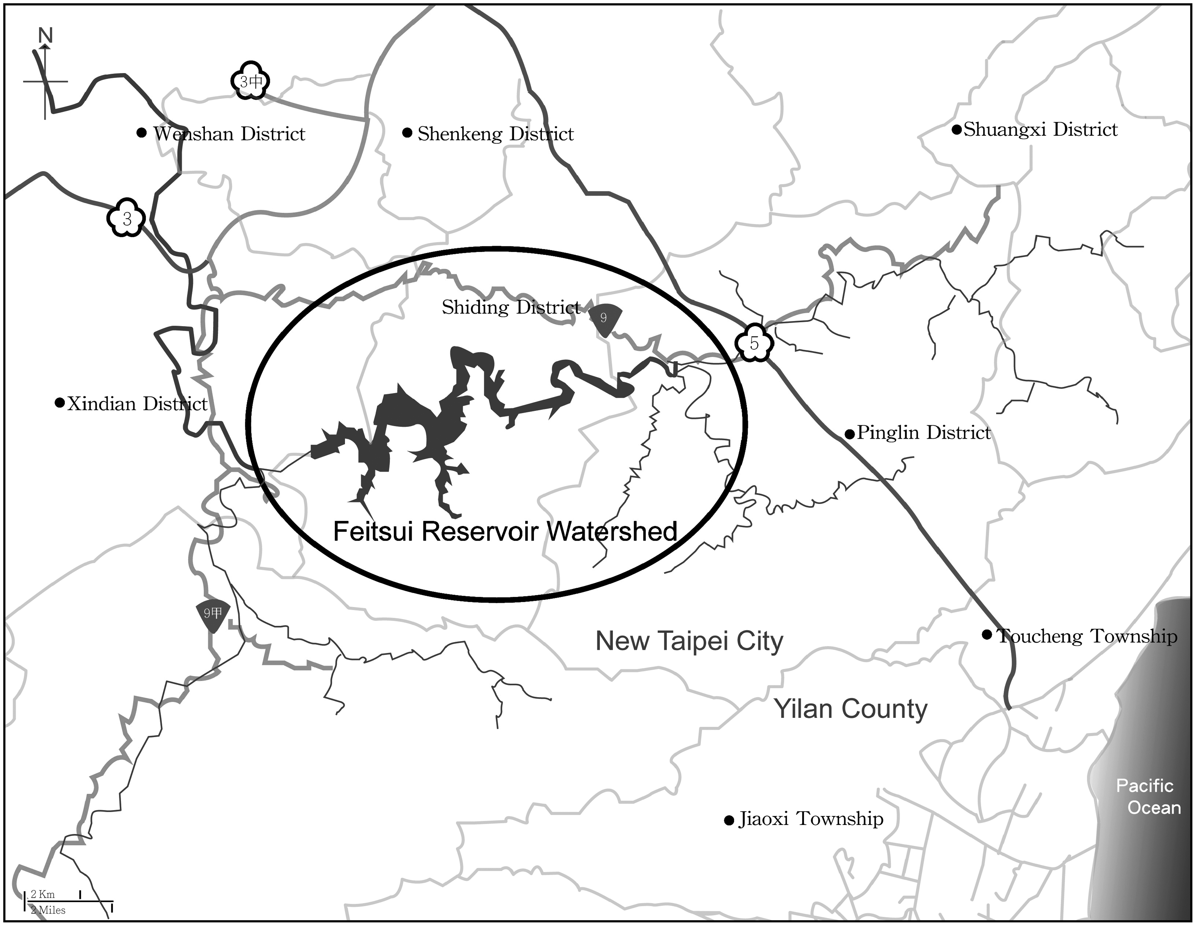
Geological location of the Feitsui reservoir watershed.

In addition, the principle component analysis method has been carried out to analyze the most obvious organic pollution factors (i.e., DO, BOD, and NH₃-N) using the VARMA model as the primary model. Hence, the correlation among various organic pollution factors can be examined to strengthen the correlation analyses of the various water quality parameters so that the time-dependent mutual influence of the these water quality parameters and the final impact can be investigated. There has not been any literature published in international journals on similar GARCH applications in environmental engineering for studying the time series variation of water quality parameters and the mutual reactions among these parameters. In this article, the statistical technology is used to assist in developing models for simulating and predicting the water quality in the watershed of northern Taiwan; the evaluation will include the test, examination, and analyses. In addition, the results obtained using the multiple statistical analyses are discussed. Because of the article length limitation, the concept and methodology of multivariate statistical method will not be covered in this article.

Methodology

ARMA modeling

A time series {x_t; t=0,±1,±2,…} is ARMA(p,q) if it is covariance stationary and can be represented as (Shumway and Stoffer, 2006) \documentclass{aastex}\usepackage{amsbsy}\usepackage{amsfonts}\usepackage{amssymb}\usepackage{bm}\usepackage{mathrsfs}\usepackage{pifont}\usepackage{stmaryrd}\usepackage{textcomp}\usepackage{portland, xspace}\usepackage{amsmath, amsxtra}\pagestyle{empty}\DeclareMathSizes{10}{9}{7}{6}\begin{document} \begin{align*} x_t = \phi_1 x_{t - 1} + \ldots + \phi_p x_{t - p} + \varepsilon_t + \theta_1 \varepsilon_{t - 1} + \ldots + \theta_q \varepsilon_{t - q} \tag{1} \end{align*} \end{document}

with ϕ_p≠0, θ_q≠0, and ɛ_t are the innovations with N(0, \documentclass{aastex}\usepackage{amsbsy}\usepackage{amsfonts}\usepackage{amssymb}\usepackage{bm}\usepackage{mathrsfs}\usepackage{pifont}\usepackage{stmaryrd}\usepackage{textcomp}\usepackage{portland, xspace}\usepackage{amsmath, amsxtra}\pagestyle{empty}\DeclareMathSizes{10}{9}{7}{6}\begin{document} $$\sigma_{\varepsilon}^2$$ \end{document} ) and \documentclass{aastex}\usepackage{amsbsy}\usepackage{amsfonts}\usepackage{amssymb}\usepackage{bm}\usepackage{mathrsfs}\usepackage{pifont}\usepackage{stmaryrd}\usepackage{textcomp}\usepackage{portland, xspace}\usepackage{amsmath, amsxtra}\pagestyle{empty}\DeclareMathSizes{10}{9}{7}{6}\begin{document} $$\sigma_{\varepsilon}^2 > 0$$ \end{document} . The parameters p and q are called the autoregressive [AR(p)] and the moving average [MA(q)] orders, respectively. When a time series does not appear covariance stationary, the differencing procedure may be applied to make it stationary. Then, the ARMA(p,q) model can be applied to the stationary differenced time series and the model so constructed is called ARIMA(p,d,q) model, where d denotes the order of differencing (Brockwell and Davis, 2002; Shumway and Stoffer, 2006). The parameters p and q have been estimated using maximum likelihood method (Brockwell and Davis, 2002) in the present study.

An inspection of autocorrelation function (ACF) and partial autocorrelation function (PACF) helps in identifying the orders AR(p) and MA(q). In addition, more objectively defined criteria such as Akaike information criterion (AIC), Hannon-Quinn information criterion, Bayesian information criterion, and final prediction error can also be used to identify the correct orders p and q (Brockwell and Davis, 2002; Kumar and Jain, 2009).

Autoregressive Conditional Heteroskedasticity

The ARCH model, which was first introduced by Engle (1982) and later extended by many researchers, has been extensively applied by Bollerslev et al. (1992), Bera and Higgins (1993), and Diebold and Lopez (1995). In contrast with the aforementioned historical volatility models, the ARCH model and its modifications do not use the sample standard deviations; they formulate conditional variance (h_t) of asset returns using the maximum likelihood procedure, which is illustrated by first defining r_t as follows: \documentclass{aastex}\usepackage{amsbsy}\usepackage{amsfonts}\usepackage{amssymb}\usepackage{bm}\usepackage{mathrsfs}\usepackage{pifont}\usepackage{stmaryrd}\usepackage{textcomp}\usepackage{portland, xspace}\usepackage{amsmath, amsxtra}\pagestyle{empty}\DeclareMathSizes{10}{9}{7}{6}\begin{document} \begin{align*} r_{\rm t} = \mu + \varepsilon_t , \tag{2} \end{align*} \end{document}

ɛ_t is defined as \documentclass{aastex}\usepackage{amsbsy}\usepackage{amsfonts}\usepackage{amssymb}\usepackage{bm}\usepackage{mathrsfs}\usepackage{pifont}\usepackage{stmaryrd}\usepackage{textcomp}\usepackage{portland, xspace}\usepackage{amsmath, amsxtra}\pagestyle{empty}\DeclareMathSizes{10}{9}{7}{6}\begin{document} \begin{align*} \varepsilon_t = \sqrt{h_t} z_t \tag{3} \end{align*} \end{document}

The distribution D is often assumed to be normal; the process z_t is scaled by h_t, a conditional variance that in turn is a function of the previous square of residual returns. In the ARCH(q) process proposed by Engle (1982), \documentclass{aastex}\usepackage{amsbsy}\usepackage{amsfonts}\usepackage{amssymb}\usepackage{bm}\usepackage{mathrsfs}\usepackage{pifont}\usepackage{stmaryrd}\usepackage{textcomp}\usepackage{portland, xspace}\usepackage{amsmath, amsxtra}\pagestyle{empty}\DeclareMathSizes{10}{9}{7}{6}\begin{document} \begin{align*} h_t = w + \sum\nolimits_{j = 1}^q \alpha_j \varepsilon_{t - j}^2 \tag{4} \end{align*} \end{document}

Conditions w>0 and α_j ≥0 are set to ensure strictly positive variance. Typically, q is of high order because of the phenomenon of volatility persistence in financial markets. From Equation (4), h_t is known at time t−1. So the “one-step ahead” forecast is readily available. The “multistep ahead” forecasts can be formulated by assuming \documentclass{aastex}\usepackage{amsbsy}\usepackage{amsfonts}\usepackage{amssymb}\usepackage{bm}\usepackage{mathrsfs}\usepackage{pifont}\usepackage{stmaryrd}\usepackage{textcomp}\usepackage{portland, xspace}\usepackage{amsmath, amsxtra}\pagestyle{empty}\DeclareMathSizes{10}{9}{7}{6}\begin{document} \begin{align*} E \big [ \varepsilon_{t + \tau}^2 \big ] = h_{t + \tau} \tag{5} \end{align*} \end{document}

The unconditional variance, r_t, is defined as \documentclass{aastex}\usepackage{amsbsy}\usepackage{amsfonts}\usepackage{amssymb}\usepackage{bm}\usepackage{mathrsfs}\usepackage{pifont}\usepackage{stmaryrd}\usepackage{textcomp}\usepackage{portland, xspace}\usepackage{amsmath, amsxtra}\pagestyle{empty}\DeclareMathSizes{10}{9}{7}{6}\begin{document} \begin{align*} \sigma^2 = \frac {\omega} {1 - \sum_{j = 1}^q \alpha_j} \tag {6} \end{align*} \end{document}

The process is covariance stationary if and only if the sum of the autoregressive parameters, \documentclass{aastex}\usepackage{amsbsy}\usepackage{amsfonts}\usepackage{amssymb}\usepackage{bm}\usepackage{mathrsfs}\usepackage{pifont}\usepackage{stmaryrd}\usepackage{textcomp}\usepackage{portland, xspace}\usepackage{amsmath, amsxtra}\pagestyle{empty}\DeclareMathSizes{10}{9}{7}{6}\begin{document} $$\sum\nolimits_{j = 1}^q \alpha_j$$ \end{document} , is less than one (<1).

Generalized ARCH

The high-order ARCH(q) process is more parsimonous to model volatility than a GARCH (Bollerslev, 1986) known as GARCH(p,q), in which additional dependencies are permitted on p lags of past h as shown as follows: \documentclass{aastex}\usepackage{amsbsy}\usepackage{amsfonts}\usepackage{amssymb}\usepackage{bm}\usepackage{mathrsfs}\usepackage{pifont}\usepackage{stmaryrd}\usepackage{textcomp}\usepackage{portland, xspace}\usepackage{amsmath, amsxtra}\pagestyle{empty}\DeclareMathSizes{10}{9}{7}{6}\begin{document} \begin{align*} h_t = \omega + \mathop\sum_{i = 1}^p \beta_i h_{t - i} \mathop\sum_{j = 1}^q \alpha_j \varepsilon_{t - j}^2 \tag{7} \end{align*} \end{document}

where h_t is in general a nonnegative random variable, and ω>0.

For GARCH(1,1), constraints α₁ ≥0 and β₁ ≥0 are needed to ensure that h_t is strictly positive. For higher orders of GARCH, the constraints on β_i and α_j are more complex. The unconditional variance σ² is expressed as \documentclass{aastex}\usepackage{amsbsy}\usepackage{amsfonts}\usepackage{amssymb}\usepackage{bm}\usepackage{mathrsfs}\usepackage{pifont}\usepackage{stmaryrd}\usepackage{textcomp}\usepackage{portland, xspace}\usepackage{amsmath, amsxtra}\pagestyle{empty}\DeclareMathSizes{10}{9}{7}{6}\begin{document} \begin{align*} \sigma^2 = \frac {\omega} {1 - \sum_{i = 1}^p \beta_i - \sum_{j = 1}^q \alpha_j} \tag {8} \end{align*} \end{document}

Additionally, the GARCH(p,q) model is covariance stationary if and only if \documentclass{aastex}\usepackage{amsbsy}\usepackage{amsfonts}\usepackage{amssymb}\usepackage{bm}\usepackage{mathrsfs}\usepackage{pifont}\usepackage{stmaryrd}\usepackage{textcomp}\usepackage{portland, xspace}\usepackage{amsmath, amsxtra}\pagestyle{empty}\DeclareMathSizes{10}{9}{7}{6}\begin{document} \begin{align*} \sum \nolimits_{i = 1}^p \beta_i + \sum \nolimits_{j = 1}^q \alpha_j < 1 \tag{9} \end{align*} \end{document}

VARMA–GARCH model

The VARMA–GARCH model of Ling and McAleer (2003) assuming symmetry in the effect of positive and negative shocks on the conditional volatility is given by \documentclass{aastex}\usepackage{amsbsy}\usepackage{amsfonts}\usepackage{amssymb}\usepackage{bm}\usepackage{mathrsfs}\usepackage{pifont}\usepackage{stmaryrd}\usepackage{textcomp}\usepackage{portland, xspace}\usepackage{amsmath, amsxtra}\pagestyle{empty}\DeclareMathSizes{10}{9}{7}{6}\begin{document} \begin{align*} Y_t = E (Y_t F_{t - 1}) + \varepsilon_t \tag{10} \end{align*} \end{document} \documentclass{aastex}\usepackage{amsbsy}\usepackage{amsfonts}\usepackage{amssymb}\usepackage{bm}\usepackage{mathrsfs}\usepackage{pifont}\usepackage{stmaryrd}\usepackage{textcomp}\usepackage{portland, xspace}\usepackage{amsmath, amsxtra}\pagestyle{empty}\DeclareMathSizes{10}{9}{7}{6}\begin{document} \begin{align*} \Psi (L) (Y_t - \mu) = \Phi (L) \varepsilon_t \tag{11} \end{align*} \end{document} \documentclass{aastex}\usepackage{amsbsy}\usepackage{amsfonts}\usepackage{amssymb}\usepackage{bm}\usepackage{mathrsfs}\usepackage{pifont}\usepackage{stmaryrd}\usepackage{textcomp}\usepackage{portland, xspace}\usepackage{amsmath, amsxtra}\pagestyle{empty}\DeclareMathSizes{10}{9}{7}{6}\begin{document} \begin{align*} \varepsilon_t = D_t \eta_t \tag{12} \end{align*} \end{document} \documentclass{aastex}\usepackage{amsbsy}\usepackage{amsfonts}\usepackage{amssymb}\usepackage{bm}\usepackage{mathrsfs}\usepackage{pifont}\usepackage{stmaryrd}\usepackage{textcomp}\usepackage{portland, xspace}\usepackage{amsmath, amsxtra}\pagestyle{empty}\DeclareMathSizes{10}{9}{7}{6}\begin{document} \begin{align*} H_t = W_t + \mathop\sum_{l = 1}^r A_l {\mathop{\varepsilon} \limits^{\rightarrow}}_{t - 1} + \mathop\sum_{l = 1}^s B_l H_{i , t - j} \tag{13} \end{align*} \end{document}

where \documentclass{aastex}\usepackage{amsbsy}\usepackage{amsfonts}\usepackage{amssymb}\usepackage{bm}\usepackage{mathrsfs}\usepackage{pifont}\usepackage{stmaryrd}\usepackage{textcomp}\usepackage{portland, xspace}\usepackage{amsmath, amsxtra}\pagestyle{empty}\DeclareMathSizes{10}{9}{7}{6}\begin{document} $$Y_t = (y_{1t} , \ldots y_{mt})^{\prime}$$ \end{document} , F_t₋₁ is the past information available up to time t, m is the total of returns to be analyzed, and t=1, …, m. L is the lag operator; \documentclass{aastex}\usepackage{amsbsy}\usepackage{amsfonts}\usepackage{amssymb}\usepackage{bm}\usepackage{mathrsfs}\usepackage{pifont}\usepackage{stmaryrd}\usepackage{textcomp}\usepackage{portland, xspace}\usepackage{amsmath, amsxtra}\pagestyle{empty}\DeclareMathSizes{10}{9}{7}{6}\begin{document} $$\Psi (L) = I_m - \Psi_1 L - \ldots - \Psi_P L^P , \ \Phi (L) = I_m - \Phi_1 L - \ldots - \Phi_q L^q$$ \end{document} , and polynomials in L. \documentclass{aastex}\usepackage{amsbsy}\usepackage{amsfonts}\usepackage{amssymb}\usepackage{bm}\usepackage{mathrsfs}\usepackage{pifont}\usepackage{stmaryrd}\usepackage{textcomp}\usepackage{portland, xspace}\usepackage{amsmath, amsxtra}\pagestyle{empty}\DeclareMathSizes{10}{9}{7}{6}\begin{document} $$D_t = {\rm diag} \ \left(h_{i , t}^{1 / 2} \right) , \ \eta_t = (\eta_{it} , \ldots , \eta_{mt})^{\prime}$$ \end{document} is a sequence of independently and identically (iid) random vectors. \documentclass{aastex}\usepackage{amsbsy}\usepackage{amsfonts}\usepackage{amssymb}\usepackage{bm}\usepackage{mathrsfs}\usepackage{pifont}\usepackage{stmaryrd}\usepackage{textcomp}\usepackage{portland, xspace}\usepackage{amsmath, amsxtra}\pagestyle{empty}\DeclareMathSizes{10}{9}{7}{6}\begin{document} $$H_t = (h_{1t} , \ldots , h_{mt})^{\prime}, \ W_1 = (\omega_{1t} , \ldots , \omega_{mt})^{\prime}, \ {\mathop{\varepsilon} \limits^{\rightarrow}}_t = (\varepsilon_{it}^2 , \ldots , \varepsilon_{mt}^2)^{\prime}$$ \end{document} , A_l, and B_l are m×m matrices with typical elements α_ij and β_ij, respectively, for i, j=1, …, m. A_l and B_l represent the ARCH effect and GARCH effect, respectively. Spillover effects or the independence of the conditional variance between West Texas Intermediate (WTI) crude oil future returns and oil company stock returns are given in conditional volatility for each return in the portfolio. Based on Equation (11), the VARMA–GARCH model also assumes that the matrix of conditional correlations is given by \documentclass{aastex}\usepackage{amsbsy}\usepackage{amsfonts}\usepackage{amssymb}\usepackage{bm}\usepackage{mathrsfs}\usepackage{pifont}\usepackage{stmaryrd}\usepackage{textcomp}\usepackage{portland, xspace}\usepackage{amsmath, amsxtra}\pagestyle{empty}\DeclareMathSizes{10}{9}{7}{6}\begin{document} $$E (\eta_t \eta_t^{\prime}) = \Gamma$$ \end{document} . If m=1, Equation (12) reduces to the univariate GARCH model of Bollerslev (1986): \documentclass{aastex}\usepackage{amsbsy}\usepackage{amsfonts}\usepackage{amssymb}\usepackage{bm}\usepackage{mathrsfs}\usepackage{pifont}\usepackage{stmaryrd}\usepackage{textcomp}\usepackage{portland, xspace}\usepackage{amsmath, amsxtra}\pagestyle{empty}\DeclareMathSizes{10}{9}{7}{6}\begin{document} \begin{align*} h_t = \omega + \mathop\sum_{i = 1}^p \alpha_i \varepsilon_{t - i}^2 + \mathop\sum_{i = 1}^q \beta_i h_{t - i}^2 \tag{14} \end{align*} \end{document}

An extension of the VARMA–GARCH model to accommodate asymmetric impacts of the positive and negative shocks is the VARMA–AGARCH model (McAleer et al., 2008) that captures asymmetric spillover effects from each of the other returns. The extension of (13) to accommodate asymmetries with respect to it ɛ is given by \documentclass{aastex}\usepackage{amsbsy}\usepackage{amsfonts}\usepackage{amssymb}\usepackage{bm}\usepackage{mathrsfs}\usepackage{pifont}\usepackage{stmaryrd}\usepackage{textcomp}\usepackage{portland, xspace}\usepackage{amsmath, amsxtra}\pagestyle{empty}\DeclareMathSizes{10}{9}{7}{6}\begin{document} \begin{align*} H_t = W_t + \mathop\sum_{l = 1}^r A_l {\mathop{\varepsilon} \limits^{\rightarrow}}_{t - 1} + \mathop\sum_{l = 1}^r C_l I (\eta_{t - l}) {\mathop{\varepsilon} \limits^{\rightarrow}}_{t - l} + \mathop\sum_{l = 1}^s B_l H_{i , t - l} \tag{15} \end{align*} \end{document}

in which \documentclass{aastex}\usepackage{amsbsy}\usepackage{amsfonts}\usepackage{amssymb}\usepackage{bm}\usepackage{mathrsfs}\usepackage{pifont}\usepackage{stmaryrd}\usepackage{textcomp}\usepackage{portland, xspace}\usepackage{amsmath, amsxtra}\pagestyle{empty}\DeclareMathSizes{10}{9}{7}{6}\begin{document} $$\varepsilon_{it} \eta \sqrt{h_{it}}$$ \end{document} for all i and t, C_l are m×m matrices and I(η_t−1) is an indicator variable, and I(η_t)=diag(I(η_t)) is an m×m matrix, such that, \documentclass{aastex}\usepackage{amsbsy}\usepackage{amsfonts}\usepackage{amssymb}\usepackage{bm}\usepackage{mathrsfs}\usepackage{pifont}\usepackage{stmaryrd}\usepackage{textcomp}\usepackage{portland, xspace}\usepackage{amsmath, amsxtra}\pagestyle{empty}\DeclareMathSizes{10}{9}{7}{6}\begin{document} \begin{align*} I (\eta_{it}) = \begin{cases}0 , \quad \varepsilon_{it} > 0 \\ 1 , \quad \varepsilon_{it} > 0\end{cases} \tag{16} \end{align*} \end{document}

If m=1, Equation (13) reduces to the asymmetric univariate GARCH or the GJR model proposed by Glosten et al. (1992): \documentclass{aastex}\usepackage{amsbsy}\usepackage{amsfonts}\usepackage{amssymb}\usepackage{bm}\usepackage{mathrsfs}\usepackage{pifont}\usepackage{stmaryrd}\usepackage{textcomp}\usepackage{portland, xspace}\usepackage{amsmath, amsxtra}\pagestyle{empty}\DeclareMathSizes{10}{9}{7}{6}\begin{document} \begin{align*} h_t = \omega + \mathop\sum_{j = 1}^r (\alpha_j + \gamma_j I (\eta_{t - j})) \varepsilon_{t - j}^2 + \mathop\sum_{j = 1}^s \beta_j h_{t - j}^2 \tag{17} \end{align*} \end{document}

If C_l=0 with A_l and B_l being diagonal matrices for all l, then VARMA–AGARCH reduces to \documentclass{aastex}\usepackage{amsbsy}\usepackage{amsfonts}\usepackage{amssymb}\usepackage{bm}\usepackage{mathrsfs}\usepackage{pifont}\usepackage{stmaryrd}\usepackage{textcomp}\usepackage{portland, xspace}\usepackage{amsmath, amsxtra}\pagestyle{empty}\DeclareMathSizes{10}{9}{7}{6}\begin{document} \begin{align*} h_t = \omega +\mathop \sum_{l = 1}^r \alpha_l \varepsilon_{i , t - l} + \mathop\sum_{l = 1}^s \beta_j h_{t - l}^2 \tag{18} \end{align*} \end{document}

which is the CCC model of Bollerslev (1990).

Essence of model development

Fat tail test

The investigation of time series empirical distribution often leads to characteristics of fat tail test. Hence, the assumption of a normal distribution for the water quality data is not the optimal choice. Results of examining the skewness, kurtosis, and Jarque-Bera normal distribution can be used for determining whether the distribution of modeling errors has fat tails.

Examination of the ARCH effectiveness

Before conducting simulations using the time series combination of ARCH and GARCH models, the process of model calibration must be carried out beforehand in order to confirm that the residual series is not related to the first order series, known as the white noise, to assure an appropriate model. Next, the residual square examination is used to determine whether the model has the (G)ARCH effect. In this article, the Q statistics proposed by Ljung-Box has been used to examine whether the residual has high-order autocorrelation. Only the model that has ARCH effectiveness can be used to carry out iterative nonlinear calculations for estimating model parameters.

Impact response analyses

The impact response analysis is used in the VAR model for studying the dynamic response pattern exhibited by all other variables when one variable is subject to exogenous shock or impulse. The development of impulse response analysis model is shown as follows (Pesaran and Shin, 1997):

The general form of VAR(m) model is \documentclass{aastex}\usepackage{amsbsy}\usepackage{amsfonts}\usepackage{amssymb}\usepackage{bm}\usepackage{mathrsfs}\usepackage{pifont}\usepackage{stmaryrd}\usepackage{textcomp}\usepackage{portland, xspace}\usepackage{amsmath, amsxtra}\pagestyle{empty}\DeclareMathSizes{10}{9}{7}{6}\begin{document} \begin{align*} \Phi (L) y_t = C + \varepsilon_t \tag{19} \end{align*} \end{document}

where y_t is an n×1 vector consisting of n variables; ɛ_t is a series of independent dynamic vibration independents with normal distribution. The average is “zero,” and the covariance matrix is Σɛ. C is an n×1 vectors with fixed values. \documentclass{aastex}\usepackage{amsbsy}\usepackage{amsfonts}\usepackage{amssymb}\usepackage{bm}\usepackage{mathrsfs}\usepackage{pifont}\usepackage{stmaryrd}\usepackage{textcomp}\usepackage{portland, xspace}\usepackage{amsmath, amsxtra}\pagestyle{empty}\DeclareMathSizes{10}{9}{7}{6}\begin{document} \begin{align*} \Phi (L) = I - \Phi_1 L - \ldots. - \Phi_m L^m \tag{20} \end{align*} \end{document}

The various Φ_S are represented by n×n matrices.

Assuming that all roots of |Φ(L)| fall outside the unit circle, the formula can be converted into Equation (21): \documentclass{aastex}\usepackage{amsbsy}\usepackage{amsfonts}\usepackage{amssymb}\usepackage{bm}\usepackage{mathrsfs}\usepackage{pifont}\usepackage{stmaryrd}\usepackage{textcomp}\usepackage{portland, xspace}\usepackage{amsmath, amsxtra}\pagestyle{empty}\DeclareMathSizes{10}{9}{7}{6}\begin{document} \begin{align*} y_t = C + \mathop\sum_{i = 1}^m \Phi_i y_{t - i} + \varepsilon_t \tag{21} \end{align*} \end{document}

It is further converted and expressed as the MA model: \documentclass{aastex}\usepackage{amsbsy}\usepackage{amsfonts}\usepackage{amssymb}\usepackage{bm}\usepackage{mathrsfs}\usepackage{pifont}\usepackage{stmaryrd}\usepackage{textcomp}\usepackage{portland, xspace}\usepackage{amsmath, amsxtra}\pagestyle{empty}\DeclareMathSizes{10}{9}{7}{6}\begin{document} \begin{align*} y_t = C + \mathop\sum_{i = 0}^{\infty} \Omega_i \varepsilon_{t - i} \tag{22} \end{align*} \end{document}

where C is an (n×1) constant matrix, Ω_i is an (n×n) matrix, and Ω₀ is a unit matrix. Equation (18) indicates that every variable in the matrix can be expressed by the ɛ_t of itself or other variables in the matrix.

Results and Discussion

Selection and manipulation of water quality data

Before the verification analysis of conditional heterogeneity variables is conducted, the water quality data collected at the six monitoring stations in the watersheds of northern Taiwan are classified into three major factors using the factor analyses in multiple statistical analyses. Factors with more significance are then selected as the targets for conducting investigations; they are termed “organic pollution factors” or factors related to pollution caused by organic pollution factor including DO, BOD, and NH₃-N.

The water quality monitoring data cover the period from January to July 2010. At first glance, the data may appear insufficient to cover a complete water quality record for the whole year. Because the watershed is located in subtropical region with the annual wet period between April and September and the annual dry period between December and March next year, the data for the specific period are sufficient to represent the typical water quality variation so that the correlations among BOD, DO, and NH₃-N can be fully grasped during the analyses. The data that show seasonal and periodic variations are normalized using the following formula before the simulation of water quality parameters is conducted: \documentclass{aastex}\usepackage{amsbsy}\usepackage{amsfonts}\usepackage{amssymb}\usepackage{bm}\usepackage{mathrsfs}\usepackage{pifont}\usepackage{stmaryrd}\usepackage{textcomp}\usepackage{portland, xspace}\usepackage{amsmath, amsxtra}\pagestyle{empty}\DeclareMathSizes{10}{9}{7}{6}\begin{document} \begin{align*} Z_{v , t} = \frac {Y_{v , t} - \mu_t} {\sigma_t} \qquad t = 1 , \ldots , w \end{align*} \end{document}

where Y_v,t are the original data; μ_t, σ_t are the periodic average and standard deviation for the data collected during the 1 – w periods.

Evaluation of water quality simulation results

The results of GARCH verification analyses confirm that using the three water quality parameters, that is, DO, BOD and NH₃-N, is appropriate.

Analyses of basic characteristics

Table 1 shows the basic characteristics of the three water quality parameters that have been evaluated for average, standard deviation, skewness, kurtosis, and Jarque-Bera normal distribution. First, as the skewness is concerned, the results indicate that BOD and NH₃-N show skew on right with positive value; BOD has the highest skewness of 2.93. This indicates that the BOD data series contains relatively more individual data with sudden increase in value. Hence, in these watersheds, BOD and NH₃-N have larger variations with respect to seasons, and BOD is more susceptible to changes of seasons. Fanchiang (2000) pointed out that the total removal efficiency of the receiving body BOD₅ may reach 65%–75% in spring and summer and 48%–51% in autumn and winter, indicating that the reduction of stream BOD is affected by the variation of temperature due to changes of seasons as seen by a right skewness of the BOD data. For DO, although both DO and water temperature vary regularly with respect to changes of seasons, the overall change degree of water quality for the watershed located in mountainous region is not as obvious as for the downstream watershed. The extent of DO variation for the former is not obvious, because its skewness is noticeable. All three water quality variations have higher kurtosis than the normal distribution, which has kurtosis of 3, indicating that these three water quality parameters have the characteristics of time sequence. Table 1 shows that BOD has a relatively higher kurtosis than the other two water quality parameters. As mentioned earlier, both BOD and NH₃-N have relatively large variations during changes of seasons; hence, they have higher kurtosis than DO. As DO is concerned, it has similar kurtosis and skewness as mentioned in previous sections, revealing that the degree of seasonal DO variation is not obviously seen. Additionally, the observations that the DO critical value (degree of freedom=2, and \documentclass{aastex}\usepackage{amsbsy}\usepackage{amsfonts}\usepackage{amssymb}\usepackage{bm}\usepackage{mathrsfs}\usepackage{pifont}\usepackage{stmaryrd}\usepackage{textcomp}\usepackage{portland, xspace}\usepackage{amsmath, amsxtra}\pagestyle{empty}\DeclareMathSizes{10}{9}{7}{6}\begin{document} $$\chi_{0.05 , 2}^2 = 5.99$$ \end{document} ) is greater than the significance level of 5% for a normal distribution support the hypothesis of rejecting the normal distribution for DO (Jarque and Bera, 1980, 1987). Further, the DO distribution has the characteristics of double thick-tail. These observations confirm that concentrations of the aforementioned water quality parameter series are easily influenced by seasons so that their concentrations vary significantly. Among the three water quality parameters, BOD has relatively the highest variations. Hence, this test confirms that BOD is more susceptible to seasonal change than NH₃-N and DO.

Table 1.

Basic Characteristics of Organic Pollution Factors

	DO (mg/L)	BOD (mg/L)	NH₃-N (mg/L)
Mean	6.713153	0.989342	0.069715
Median	6.800000	0.800000	0.040000
Maximum	8.700000	7.200000	0.450000
Minimum	3.400000	0.200000	0.010000
Std. Dev.	0.829993	0.802781	0.063600
Skewness	−0.385656	2.937852	2.407225
Kurtosis	3.36178	18.64152	10.88435
Jarque-Bera	8.288771	3268.743	999.2112
Probability	0.015853	0.000000	0.000000
Sum	1886.500	278.0000	19.5900
Sum Sq. Dev.	192.8886	180.44880	1.132577
Observations (n)	281	281	281

Ljung-box sequential examination

Prior to using the ARCH and GARCH models, the residual in the regression model is first examined using the Ljung-Box examination (L-B-Q(K)) method to test whether it has the ARCH or GARCH effect; the results are listed in Table 2. All the examination statistics for L-B-Q(K) are smaller that the critical value so that null hypothesis, which is not conforming to alternative hypothesis, cannot be rejected. Hence, residuals of the various number sequences do not have serial correlation; this confirms to the phenomenon of white noise so that the model disposition is considered appropriate.

Table 2.

Ljung-Box Serial Examinations of Organic Pollution Factors

L-B-Q(K)	DO	BOD	NH₃-N	Critical value \documentclass{aastex}\usepackage{amsbsy}\usepackage{amsfonts}\usepackage{amssymb}\usepackage{bm}\usepackage{mathrsfs}\usepackage{pifont}\usepackage{stmaryrd}\usepackage{textcomp}\usepackage{portland, xspace}\usepackage{amsmath, amsxtra}\pagestyle{empty}\DeclareMathSizes{10}{9}{7}{6}\begin{document} $$\chi_{(0.05 , k)}^2$$ \end{document}
1	0.55	0.81	0.58	3.84
2	1.26	1.37	1.12	5.99
3	3.57	3.44	2.57	7.82
4	6.68	5.89	3.06	9.49
5	9.02	7.21	6.65	11.07
6	10.44	8.94	7.98	12.59
7	12.59	11.32	9.35	14.07
8	13.67	12.80	11.00	15.51
9	14.41	15.33	12.57	16.92
10	15.58	16.72	14.81	19.68
15	22.96	20.79	17.98	26.30
20	26.31	25.08	23.67	31.41

R_t=c+θ R_t₋₁+ɛ_t; α=0.05.

DO, dissolved oxygen; BOD, biochemical oxygen demand; NH₃-N, ammonia nitrogen.

Examination of ARCH effectiveness

The Lagrange Multiplier (LM) statistics (Lee et al., 2007) can be applied to examine whether the ARCH effect exists in a number sequence. The LM statistics is TR² with T being the number of samples, and R² being the determination coefficient value obtained using the ordinary least squares (OLS) regression; TR² obeys the chi-square distribution with p degree of freedom. When the model LM statistics is obvious, the ARCH effect exists in the number sequence. The statistics of the three water quality parameters listed in Table 3 indicates that the conditional variance of all three parameters show strong ARCH effect with all TR² values less than 5% indicating “obviousness.” Hence, the ARCH effectiveness is appropriate for explaining these three water quality parameters.

Table 3.

Results of ARCH(q) Examination of Organic Pollution Factors

Q (lagged variables)	DO (TR²)	BOD (TR²)	NH₃-N (TR²)	Critical value \documentclass{aastex}\usepackage{amsbsy}\usepackage{amsfonts}\usepackage{amssymb}\usepackage{bm}\usepackage{mathrsfs}\usepackage{pifont}\usepackage{stmaryrd}\usepackage{textcomp}\usepackage{portland, xspace}\usepackage{amsmath, amsxtra}\pagestyle{empty}\DeclareMathSizes{10}{9}{7}{6}\begin{document} $$x_{(0.05 , k)}^2$$ \end{document}
1	71.59	18.82	53.20	3.84
2	88.06	24.45	64.74	5.99
3	98.86	30.84	81.00	7.82
4	113.47	33.90	94.32	9.49
5	134.11	39.82	100.32	11.07
6	147.88	49.81	143.17	12.59
7	167.43	56.33	153.89	14.07
8	189.05	69.97	170.65	15.51
9	223.32	75.21	187.58	16.92
10	255.87	88.26	201.99	19.68

All TR² values are less than 5%, indicating “obviousness.”

Selecting VARMA to cope with GARCH

In this article, various combinations of the vector model VARMA coped with ARCH–GARCH model have been tested to select the optimum VARMA(p,d,q)–GARCH(p,q) model for conducting the simulation of water quality. The results will then be appropriate for depicting the water quality parameters dependence among the various organic pollution factors. Table 4 lists the analysis results for matching VARMA with the GARCH model. Among the hundreds of various combinations of vector models, one set of the combinations, that is, VARMA(1,0,1)–GARCH(1,1), has been selected as the most appropriate model for explaining and depicting the time series dependence of the various organic pollution factor, because this combination has the smallest AIC and Schwartz criteria (SC).

Table 4.

Results of the VARMA(p,d,q)–GARCH(p,q) Examinations of Organic Pollution Factors

ARCH	ARCH(1)		GARCH(1,0)		GARCH(1,1)		GARCH(1,2)		GARCH(2,1)
VARMA	AIC	SC	AIC	SC	AIC	SC	AIC	SC	AIC	SC
VARMA(1,0,0)	2.761	2.765	2.563	2.449	2.551	2.603	2.696	2.761	2.372	2.370
VARMA(2,0,0)	2.653	2.608	2.338	2.361	2.552	2.604	2.696	2.762	2.568	2.534
VARMA(0,0,1)	2.097	1.996	2.470	2.296	2.668	2.719	2.553	2.541	2.517	2.558
VARMA(0,0,2)	1.896	1.895	2.508	2.448	0.116	−0.065	2.004	2.179	2.001	1.996
VARMA(1,0,1)	2.810	2.862	1.281	1.372	−0.230	−0.165	2.364	2.442	−0.073	−0.106
VARMA(1,0,2)	2.816	2.798	2.797	2.685	2.430	2.495	1.753	1.790	2.282	2.185
VARMA(2,0,1)	2.799	2.557	2.658	2.650	2.224	2.374	2.364	2.442	2.097	2.016

VARMA, Vector Autoregressive Moving Average; GARCH, Generalized Autoregressive Conditional Heteroskedastic; AIC, Akaike information criterion; SC, Schwartz criteria.

Values in boldface are the smallest AIC and SC values.

Simulation results using the VARMA coupled GARCH model

Table 5 lists the time series correlation and dependence among BOD, DO, and NH₃-N that have been simulated using the optimum VARMA(1,0,1)–GARCH(1,1) model. Numerous matching models have been tested in this research, and only the models that are the most appropriate for conducting the studies are explained in the following sections.

Table 5.

Values of Parameters Used in Combining VARMA and GARCH(1,1) for Organic Pollution Factors

	a₀	a₁	a₂	b₀	b₁	b₂	c₀	c₁	c₂	d₁	α₀	α₁	α₂	β₁
VARMA(1,0,0)	−0.56	−1.00		1.03	0.55		0.88	0.62			4.65	−4.65	0.27	0.06
t-statistic	1.91	0.27		−0.24	1.37		−2.65	−1.23			1.23	3.99	0.54	−1.12
VARMA(2,0,0)	−1.32	2.37		0.56	0.98	−1.18	−2.36	−0.87	−0.92	0.65	0.65	2.65	0.85	0.67
t-statistic	−0.88	2.01		1.09	−2.37	0.54	1.33	0.67	1.01	1.22	0.99	2.12	−0.23	1.03
VARMA(0,0,1)	1.10			0.76			0.54			1.11	1.56	−0.76	1.64	1.26
t-statistic	2.45			−2.27			−0.29			−0.24	2.33	0.24	−0.68	2.38
VARMA(0,0,2)	0.92		1.03	1.28			0.06	0.34	1.00	0.11	1.32	1.09	1.23	0.56
t-statistic	−0.07		0.80	−1.38			1.32	−0.67	2.34	1.37	−0.98	−0.86	−0.93	0.33
VARMA(1,0,1)	2.56	0.58	4.37	−0.71	1.20	0.95	3.55	−1.27	0.17		7.88	−1.25	0.28	2.44
t -statistic	6.36	9.62	−2.07	3.14	3.59	−2.43	0.97	2.58	−2.26		2.49	3.93	1.25	12.52
VARMA(1,0,2)	1.13	0.87	0.23	1.23	0.54		1.99	1.20	−0.56		3.87	−0.87	2.38	−0.87
t-statistic	0.67	−0.92	−0.91	−0.90	1.07		−0.20	2.87	0.23		2.78	−0.53	1.90	−0.06
VARMA(2,0,1)	−2.54	−1.02		1.96	−0.07	1.76	−2.23	1.09	2.36		−0.54	2.22	1.75	−0.54
t-statistic	1.14	−0.99		2.67	0.14	0.87	1.78	−0.07	1.09		0.71	−1.45	0.76	0.27

\documentclass{aastex}\usepackage{amsbsy}\usepackage{amsfonts}\usepackage{amssymb}\usepackage{bm}\usepackage{mathrsfs}\usepackage{pifont}\usepackage{stmaryrd}\usepackage{textcomp}\usepackage{portland, xspace}\usepackage{amsmath, amsxtra}\pagestyle{empty}\DeclareMathSizes{10}{9}{7}{6}\begin{document} $${\rm BBOD} = a_0 + a_1 \ {\rm BOD}_{(t - 1)} + a_2 \ {\rm BOD}_{(t - 2)} + b_0 \ {\rm DO}_{(t)} + b_1 \ {\rm DO}_{(t - 1)} + b_2 \ {\rm DO}_{(0t - 2)} + c_0 \ {\rm NH}_3 \hbox{-} {\rm N}_{(t)} + c_1 \ {\rm NH}_3 \hbox{-} {\rm N}_{(t - 1)} + c_2 \ {\rm NH}_3 \hbox{-} {\rm N}_{(t - 2)} + d_1 \varepsilon_{t - 1} h_t = \alpha_0 + \alpha_1 \varepsilon_{t - 1}^2 + \alpha_2 \varepsilon_{t - 2}^2 + \beta_1 h_{t - 1}$$ \end{document}

Values in boldface were used to execute the simulation.

As the DO is concerned, the simulated results shown in Table 5 reveal that the current stream DO will affect the formation of BOD concentration (t-statistics of b₀ of 3.14 is greater than 1.96, indicating “significant”). That is, the magnitude of current stream DO variation can be applied for predicting the current concentration of BOD; this can also be verified by the results obtained using the BOD equation, where DO_i is the initial sample DO, DO_f is the sample DO after 5-day incubation period, and P is the dilution factor. In Table 5, b₀ value of the current DO is −0.71, indicating that when the stream water contains relatively high DO, the BOD can be completely degraded by consuming and reducing the stream DO. Additionally, the one time lag and two times lag DO values will also influence the concentration of BOD formation (t-statistics of b₁ and b₂ are 3.59 and −2.43, respectively, both being greater than 1.96, indicating “significant”). Further, the one time lag and two times lag DO values influence the current BOD more than the current DO [both b₁(1.20) and b₂(0.95) have a greater coefficient than b₀(−0.71)]. The above observations illustrate that aerobic microbes consume more DOs during one time lag and two times lag than the current consumption of DO. This is also confirmed by the first derivative of the oxygen sag curve based on Streeter-Phelps equation (Lo, 2004).

The current BOD is mostly caused by the degradation of carbonaceous organic matter; it is also known as the carbonaceous BOD (BOD_C), whereas the oxygen consumption in the nitrification (or oxidation) of NH₃-N contributes to nitrogenous BOD (BOD_N). The stream total BOD is the sum of BOD_C and BOD_N. Because nitrifying microbes have smaller specific growth rates than normal BOD_C oxidizing microbes, the reduction of BOD_N comes after the reduction of BOD_C. When NH₃-N is concerned, the simulated results listed in Table 5 indicate that the current NH₃-N concentration cannot be used for predicting the current concentration of carbonaceous BOD formation (t-statistic of c₀ being 0.97 is smaller than 1.96, indicating “not significant”). However, both the one time lag and two times lag NH₃-N concentrations affect the nitrogenous BOD formation (t-statistic of c₁, and c₂ being 2.58, and −2.26, respectively, which are greater than 1.96, indicating “significant”). The above analyses show that the current BOD_N concentration is influenced by the one time lag and two times lag NH₃-N concentrations. This observation can be explained based on the production of the decomposition of the organic matter containing nitrogen. Right after the stream is polluted by discharges of domestic wastewater, the current oxidation does not occur immediately as seen in the t-statistics of c₀ that indicates “not significant”; hence, the change of BOD concentration is not obvious. After the majority of BOD is degraded, organic nitrogen is then hydrolyzed into NH₃-N, which is then oxidized biologically into nitrite and nitrate to further consume DO. Hence, the one time lag and two times lag ammonia concentrations obviously influence the current BOD_N concentration. Further, the one time lag NH₃-N influences the current BOD more than the two times lag NH₃-N, showing that most one time lag NH₃-N has been oxidized into nitrite and nitrate nitrogen.

For BOD, it is more influenced during the one time lag period (t-statistic of a₁ being 9.62 is greater than 1.96, indicting “significant”) than the two times lag period (t-statistic of a₂ is −2.07, whose absolute value is greater than 1.96, indicting “significant”). In other words, the results indicate that BOD curve shows an initial microbial logarithmic growth so that the BOD is rapidly reduced during the one time lag period. However, the decomposition of organic matter during the two times lag period obviously decreases, which lead to slower final BOD increasing rate.

Predictive analyses using the VARMA(1,0,1)–GARCH(1,1)

Predicting future variations is very important in time series model. In this study, the final 30 sets of data collected on the three water quality items have been used for conducting the time series simulating prediction using the VARMA(1,0,1)–GARCH(1,1) model. The prediction results are shown in Figs. 2 –4. All three water quality parameters have high coefficient of correlation r between the fitted and actual values, that is, 0.813 for DO, 0.986 for BOD, and 0.905 for NH₃-N. Hence, these three water quality parameters have characteristics of timer sequence so that they can be accurately predicted using the GARCH model as developed in this research.

FIG. 2.

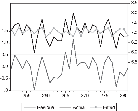
Results of predicting DO using the VARMA(1,0,1)–GARCH(1,1) model. DO, dissolved oxygen; VARMA, Vector Autoregressive Moving Average; GARCH, Generalized Autoregressive Conditional Heteroskedastic.

FIG. 3.

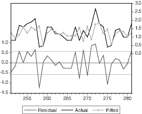
Results of predicting biochemical oxygen demand using the VARMA(1,0,1)–GARCH(1,1) model.

FIG. 4.

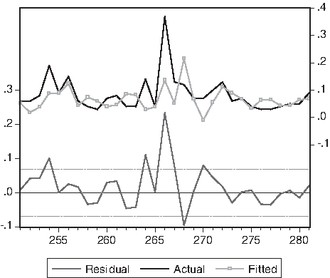
Results of predicting NH₃-N using the VARMA (1,0,1)–GARCH(1,1) model. NH₃-N, ammonia nitrogen.

Impact response analyses

Before the impact response analysis is conducted, the number of period for the most appropriate lagged variable must be selected (Kane and Unal, 1990). The test results using three unit root test models show that the original data for these three water quality parameters cannot reject null presumption unit root; hence, they are nonstationary sequence. If the number of period for the selected lagged variables is too short, the resulting simplification will miss the specified results. On the contrary, if the number of period is too long, the excessively detained parameters will cause inefficient estimation of the parameters. Hence, a reliable criterion may be determined for selecting an appropriate number of the lagged period for effectively reducing estimation errors and raising model efficiency.

The AIC proposed by Akaike is used in this article for selecting appropriate lagged variables: \documentclass{aastex}\usepackage{amsbsy}\usepackage{amsfonts}\usepackage{amssymb}\usepackage{bm}\usepackage{mathrsfs}\usepackage{pifont}\usepackage{stmaryrd}\usepackage{textcomp}\usepackage{portland, xspace}\usepackage{amsmath, amsxtra}\pagestyle{empty}\DeclareMathSizes{10}{9}{7}{6}\begin{document} \begin{align*} {\rm AIC} (m) = T \times \ln ({\rm SSR} / T) + 2m \end{align*} \end{document}

where m is the number of variables in a model, T is the number of samples, and SSR is the sum of error squares.

The AIC of lagged variable are first tested for selecting the one with the smallest AIC value as the most appropriate lagged variable to be used as the basis for analyses. The results shown in Table 6 indicate that the lagged variable in the ninth period has smaller AIC value. Hence, the ninth lagged variable is selected for conducting the impact response analyses for the three water quality variables. Figure 5 shows the impact response when the three water quality parameters produce a unit variation.

FIG. 5.

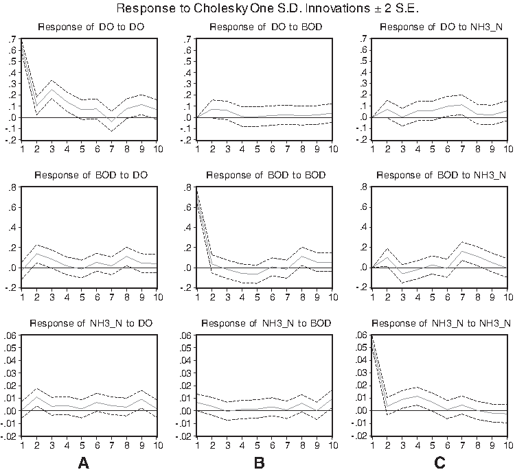
Impact response analyses for organic pollution factors: (A) response to DO; (B) response to BOD; (C) response to NH₃-N. The dashed line represents the range of impact response degree. The gray line represents average value of impact response degree.

Table 6.

Time Lag Akaike Information Criterion Value of Organic Pollution Factor

Lag items	AIC
1	−2.75
2	−3.03
3	−2.98
4	−3.05
5	−3.32
6	−2.54
7	−2.56
8	−3.07
9	−3.61
10	−3.49

For DO, Fig. 5A shows the impact responses of BOD and NH₃-N to variations of DO. The results indicate that BOD responses immediately to changes of current DO. This observation conforms to the previous conclusion that the current stream DO will influence the concentration of BOD formation (t-statistic of b₀ being 2.14 is greater than 1.96, indicating “significant”). Further, Fig. 5A also reveals that the one time lag DO influences BOD more than the current DO. This is also similar to the previous conclusion concerning the influence of DO on BOD as indicated by the VARMA(1,0,1)–GARCH(1,1) model. NH₃-N is not involved in the reaction as soon as the current DO varies, because NH₃-N in water is oxidized into either NO₂ or NO₃, so that the existence of NH₃-N in the water usually indicates little or no nitrification oxidation reactions. Hence, the variation of current DO does not mean that NH₃-N is involved in the oxidation reaction; the current DO cannot be based on for predicting the current NH₃-N concentration. The results shown in Fig. 5A reveal that oxidation of NH₃-N does not occur until the one time lag DO begins to change. The oxidation of NH₃-N leads to the formation of nitrites or nitrates; the change of NH₃-N is also obviously influenced by the change of the two times lag DO concentration.

For BOD, impact responses of DO and NH₃-N to BOD variation are shown in Fig. 5B. The figure reveals that DO reduction is not obvious as soon as the current BOD starts to change. Only when the microbial growth enters the log-phase, DO consumption increases logarithmically so that BOD reduction becomes obvious. Additionally, NH₃-N starts to react when the current carbonaceous BOD is almost oxidized, because the nitrification oxidation reaction does not occur immediately after the river has been freshly polluted by domestic wastewater discharges. When BOD is observed later, NH₃-N has already been oxidized into nitrites or nitrates. Fig. 5B also reveals that the total BOD is obviously affected by the current carbonaceous BOD and the one time lag nitrogenous BOD concentrations. Higher current BOD concentrations indicate more serious pollution to consume more DO and a longer period for the stream to recover. This observation is similar to the results obtained using the VARMA(1,0,1)–GARCH(1,1) model (t-statistic of a₂ being negative is smaller than the t-statistic of a₁).

For NH₃-N, the impact response of DO and BOD to variation of NH₃-N is shown in Fig. 5C. The results indicated that as soon as the NH₃-N starts to change, the current DO does not response until the one time lag is reached. As mentioned earlier, NH₃-N originates from the biological decomposition of nitrogen-containing organic matter in the domestic wastewater discharge. During the initial stage of NH₃-N decomposition, the consumption of DO is not obvious, and during the one time lag period, NH₃-N is further oxidized into nitrite and nitrate to make the increase of DO consumption more obvious. Nitrification usually occurs at the time when most carbonaceous BOD is almost exhausted; hence, BOD does not change obviously until when the current NH₃-N begins to change, which contributes to nitrogenous BOD (BOD_N). These results are similar to the simulated results presented earlier using the VARMA(1,0,1)–GARCH(1,1) model that the current NH₃-N concentration cannot be applied for estimating the current BOD (t-statistic of c₀ being 0.97 is smaller than 1.96, indicating “not significant”). Hence, the moment when NH₃-N starts to vary, the current NH₃-N concentration does not affect the current carbonaceous BOD concentration. During the one time lag period, the current total BOD concentration is affected by the current NH₃-N concentration, which contributes to nitrogenous BOD.

Conclusion

Model analyses on the three water parameters (i.e., BOD, DO, and NH₃-N) that have been selected based on the result of multivariable statistical analyses have been conducted using the water quality monitoring data collected at six tributary streams of Feitsui reservoir watershed. ARCH and GARCH effects exist in the BOD, DO, and NH₃-N, because these water quality parameters have a tendency to change with respect to changes of seasons. In other words, a previous change of water parameters will cause the current water parameters to vary accordingly.

The results obtained in this research show that both BOD and NH₃-N skew to the right; BOD has the highest skewness of 2.93, indicating that many individual BOD data in the series of BOD data show the phenomenon of sudden increase. Hence, the BOD and NH₃-N in the watershed in question show great seasonal variations. Based on the normal distribution statistics (Jarque-Bera), their 5% levels are greater than the critical boundary value (degree of freedom of 2 and \documentclass{aastex}\usepackage{amsbsy}\usepackage{amsfonts}\usepackage{amssymb}\usepackage{bm}\usepackage{mathrsfs}\usepackage{pifont}\usepackage{stmaryrd}\usepackage{textcomp}\usepackage{portland, xspace}\usepackage{amsmath, amsxtra}\pagestyle{empty}\DeclareMathSizes{10}{9}{7}{6}\begin{document} $$x_{0.05 , 2}^2 = 5.99$$ \end{document} ). The normal distribution shows the characteristic of double fat tails to reveal that the water quality is easily influenced by seasons.

Results of simulation using the optimum matching VARMA(1,0,1)–GARCH(1,1) model show that the one time lag and two time lab NH₃-N concentrations affect the current BOD. This is seen by the statistical analysis results obtained in this study that the total BOD is influenced by the current carbonaceous BOD (BOD_C) and one time lag nitrogenous BOD (BOD_N). In this research, results of impact response studies indicate that NH₃-N does not significantly involve in the reaction when DO starts to change because of the low specific growth nature of nitrifying microbes. The presence of NH₃-N indicates that the current nitrification oxidation has not occurred or has completed. Variation of DO in the water body after most carbonaceous BOD has been oxidized indicates the oxidation of NH₃-N. Hence, the water body DO concentration cannot be used for predicting the immediate current NH₃-N concentration. The research results also show that when carbonaceous BOD (BOD_C) starts to change, NH₃-N is not significantly oxidized. Later, the carbonaceous BOD does not involve in the reaction when the current NH₃-N concentration is oxidized to contribute to the one time lag nitrogenous BOD.

The VARMA–GARCH integrated model proposed in this research will have a complete grasp of instantaneous changes of the time series water quality in the watershed so that the previous practice of ignoring the changes of series water quality is improved. The results will provide valuable references for the water quality authority to implement timely and effective water management measures in response to changes of water quality.

Footnotes

Acknowledgments

The authors sincerely appreciate financial support for the project (NSC 100-2221-E214-011) from Taiwan's National Science Council for the work. The authors also deeply appreciate the anonymous reviewers for their insight comments and suggestions.

Author Disclosure Statement

No competing financial interests exist.

References

Bera

, Higgins

B.K.

1993. ARCH models: properties, estimation and testing. J. Econ. Surv., 7:305.

Bollerslev

1986. Generalized autoregressive conditional heteroskedasticity. J. Econom., 31:307.

Bollerslev

1990. Modelling the coherence in short-run nominal exchange rate: a multivariate generalized ARCH approach. Rev. Econ. Stat., 72:498.

Bollerslev

, Chou

R.Y.

, Kroner

K.F.

1992. ARCH modeling in finance. J. Econom., 52:5.

Brockwell

J.B.

, Davis

R.A.

2002. Introduction to Time Series and Forecasting. New York: Springer-Verlag, Inc.

Cobourn

W.G.

2007. Accuracy and reliability of an automated air quality forecast system for ozone in seven Kentucky metropolitan areas. Atmos. Environ., 41:5863.

Diebold

F.X.

, Lopez

1995. Modeling volatility dynamics. Kevin

Hoover

. Macroeconometrics: Developments, Tensions and Prospects. Boston: Kluwer Academic Publishers, 427.

Engle

1982. Autoregressive conditional heteroskedasticity with estimates of the variance of U.K. inflation. Econometrica, 50:987.

Fanchiang

R.M.

2000. Body of Biodegradability Enhancement for Industrial Wastewater by Preozonation Process [Master's Thesis] Environmental Engineering Research Institute, National Central University: Taipei, Taiwan(In Chinese.)

10.

Glosten

, Jagannathan

, Runkle

1992. On the relation between the expected value and volatiltiy and of the nominal excess returns on stocks. J. Finance, 46:1779.

11.

Hoti

S.M.

, McAleer

, Chan

2005a. Modelling the spillover effects in the volatility of atmospheric carbon dioxide concentrations. Math. Comput. Simulation, 69:46.

12.

Hoti

S.M.

, McAleer

, Pauwels

2005b. Modelling risk spillovers in environmental finance. Proceedings of the 2005 International Conference on Simulation and Modelling, Thailand. Asian Institute of Technology0,498.

13.

Hoti

S.M.

, McAleer

, Pauwels

2008. Multivariate volatility in environmental finance. Math. Comput. Simulation, 78:189.

14.

Hubbard

M.C.

, Cobourn

M.C.

1998. Development of a regression model to forecast ground-level ozone concentration in Louisville, KY. Atmos. Environ., 32:2637.

15.

Jarque

C.M.

, Bera

A.K.

1980. Efficient tests for normality, homoscedasticity and serial independence of regression residuals. Econ. Lett., 6:255.

16.

Jarque

C.M.

, Bera

A.K.

1987. A test for normality of observations and regression residuals. Int. Stat. Rev., 55:163.

17.

Kane

E.J.

, Unal

1990. Modeling structural and temporal variation in the market's valuation of banking firms. J. Finance, 45:113.

18.

Kumar

, Jain

V.K.

2010. ARIMA forecasting of ambient air pollutants (O₃, NO, NO₂ and CO) Stoch. Env. Res. Risk A., 24:751.

19.

Lee

C.L.

, Lee

R.K.

, Kao

Y.M.

2007. Lagrange multiplier optimization synthesis of long-period fiber gratings. National Tsing Hua University Institutional Repository. Institute of Electrical and Electronics Engineers, EE Conference Papers: Hsinchu City, Taiwan(In Chinese.)

20.

Ling

, McAleer

2003. Asymptotic theory for a vector ARMA-GARCH model. Econom. Theory, 19:109.

21.

S.L.

2004. Environmental Mathematics. Taiwan: Maw Chang Book Co., Ltd(In Chinese.)

22.

McAleer

2005. Automated inference and learning in modeling financial volatility. Econom. Theory, 21:232.

23.

McAleer

, Chan

, Hoti

, Lieberman

2008. Generalized autoregressive conditional correlation. Econom. Theory, 24:1554.

24.

Pesaran

M.H.

, Shin

1997. Generalized impulse response analysis in linear multivariate models. J. Econom., 58:117.

25.

Serletis

, Shahroradi

2006. Measuring and testing natural gas and electricity markets volatility: evidence from Alberta's deregulated Markets. CERI Working Papers on Energy, Environment and the Economy, University of Calgary: Canada, 1.

26.

Shumway

R.H.

, Stoffer

D.S.

2006. Time Series Analysis and Its Applications—with R Examples. Hamburg, Germany: Springer Science+Business Media, LLC.

27.

Slini

, Karatzas

, Moussiopoulos

2002. Statistical analysis of environmental data as the basis of forecasting: An air quality application. Sci. Total Environ., 288:227.

28.

Surgailis

, Viano

2002. Long memory properties and covariance structure of the EGARCH model. ESAIM Probab. Stat., 6:311.

29.

Tansuchat

, McAleer

, Chang

2009. Volatility spillovers between crude oil futures returns and oil company stock returns. 18th World IMACS/MODSIM Congress: Cairns, Australia, July 13–17 1356.