Practical Implementation of New Particle Tracking Method to the Real Field of Groundwater Flow and Transport

Abstract

In articles published in 2009 and 2010, Suk and Yeh reported the development of an accurate and efficient particle tracking algorithm for simulating a path line under complicated unsteady flow conditions, using a range of elements within finite elements in multidimensions. Here two examples, an aquifer storage and recovery (ASR) example and a landfill leachate migration example, are examined to enhance the practical implementation of the proposed particle tracking method, known as Suk's method, to a real field of groundwater flow and transport. Results obtained by Suk's method are compared with those obtained by Pollock's method. Suk's method produces superior tracking accuracy, which suggests that Suk's method can describe more accurately various advection-dominated transport problems in a real field than existing popular particle tracking methods, such as Pollock's method. To illustrate the wide and practical applicability of Suk's method to random-walk particle tracking (RWPT), the original RWPT has been modified to incorporate Suk's method. Performance of the modified RWPT using Suk's method is compared with the original RWPT scheme by examining the concentration distributions obtained by the modified RWPT and the original RWPT under complicated transient flow systems.

Introduction

Many particle tracking techniques have been developed to account for the advective component in the Lagrangian-Eulerian framework (Konikow et al., 1996; Zheng, 1990; Yeh et al., 1992; Clement, 1997). Nevertheless, in flow field conditions, these methods have limitations and problems, such as steady or transient flow, complexity of temporal velocity variations, adoption of either mesh refinement or in-element path refinement, numerical methods of either the finite difference method (FDM) or the finite element method (FEM), and the type of element used. Most particle tracking methods are limited to steady state flow cases (Bear and Verruijt, 1987; Cheng et al., 1996; Javandel et al., 1984; Pollock, 1988; Schafer-Perini and Wilson, 1991). MODPATH (Pollock, 1994), MOC3D (Konikow et al., 1996), MT3D (Zheng, 1990) and RT3D (Clement, 1997), are the most popular particle tracking methods. However, Pollock's method, Konikow's method, and Zheng's method employ only FDM and do not consider the changes in velocity during a time step in a complicated unsteady flow or a rapidly changing velocity field with time.

Recently, Suk and Yeh (2009, 2010) described the detailed process and algorithms of accurate and efficient particle tracking techniques, known as Suk's method, that can account for changes in velocity during a time step in a complicated unsteady flow. The complicated unsteady flow consists of a local velocity field with significant variances in both time and space under which the traditional particle tracking schemes often fail to obtain accurate travel time and path line. These traditional particle tracking schemes often fail because it is difficult to approximate mean velocities during a large time step. In particular, the complicated unsteady flow represents both temporally and spatially varying velocity fields with rapidly changing velocity. Although Suk and Yeh (2009, 2010) demonstrated the superiority of Suk's method over existing particle tracking methods, such as Pollock's method (Pollock, 1988, 1994) and Cheng's method (Cheng et al., 1996), they did not report the practical applications of the particle tracking method in a real field situation nor did they show the extensive applicability of Suk's method to such numerical methods as the random walk particle tracking method (RWPT) and the Eulerian-Lagrangian method (ELM), for solving solute transport problems that require an efficient advective particle tracking scheme.

This paper reports the practical application of Suk's method to illustrate its applicability to a real problem. In this study, the practical applicability to real problems will be shown, using two examples. First, the aquifer storage and recovery (ASR) example was chosen to show how the fronts of injected water move during the injection and recovery phases. Second, the scenario of landfill leachate migration was examined to illustrate the wider applicability and superior performance of Suk's method over Pollock's method. In addition, to show the wide applicability of Suk's method to advection-dispersion problem, the original RWPT was modified in this study to incorporate Suk's method to calculate efficient advective particle tracking. The performance of the modified RWPT was compared with the original RWPT schemes under two different complicated transient flow conditions, shown in the third and fourth examples.

Suk's Method

Suk's particle tracking method was designed to trace fictitious particles in a real-world flow field, where the flow velocity is either measured or calculated at a limited number of locations. The technique traces fictitious particles on an element to element basis. A fictitious particle is traced with a given velocity field, element by element, until either a boundary is encountered or the available time is consumed. For tracking within an element, the element is divided into a number of subelements, according to user's desire. Within the subelement, particle tracking locates the target side of the subelement and then calculates the target point and tracking time at the target side, using the algorithms proposed by Suk and Yeh (2009, 2010). This process is repeated in the element until the path line crosses the adjacent element. When particle hits the boundary of the adjacent element, particle tracking proceeds on the adjacent element. In contrast to the previous particle tracking methods, Suk's method can consider the changes in velocity during a time step to deal with complicated unsteady flow and shows better performance.

Practical Implementations

Four examples are given here to demonstrate practical implementations of Suk's method. The first two show its practical application to ASR problems and landfill leachate migration problems, which are issues in geoscience. In the third and fourth examples, to achieve improvement in the numerical performance of the original RWPT, the original RWPT was modified to incorporate Suk's method, and the numerical results of the modified RWPT are compared with the results of the original RWPT to illustrate the efficiency of the modified RWPT using Suk's method.

The ASR problem involves injecting large quantities of surface water into aquifers and recovering the stored water from the same well during periods of demand. Since the movement of water injected in the ASR includes advective and dispersive components, commonly used numerical ground water models, such as MODFLOW (Harbaugh et al., 2000), FEMWATER (Yeh et al., 1992), MT3D (Zheng, 1990) and FEFLOW (Diersch, 2006), might be needed to determine the mixing or transport behavior of the injected water. Ward et al. (2008) performed both ASR modeling, using FEFLOW, and a simulation with transient flow, and transient transport, using the forward Adams-Bashforth/backward trapezoidal predictor-corrector scheme. Lowry and Anderson (2006) used MODFLOW to simulate a flow field in response to the injection and recovery of water and then used MODPATH to track the movement of imaginary particles by advection at the average linear velocity generated by MODFLOW. They used either MODPATH or MT3D to evaluate the relative effect of hydraulic or operational factors, such as the hydraulic gradient, longitudinal dispersivity, and storage period, on the recovery efficiency. They concluded that compared to the solute transport models, particle tracking simulations can overpredict the recovery rates by as much as 30%. Therefore, the use of particle tracking models should be limited to sites where the injected and ambient water are of the same chemistry or when mixing is not an issue. When mixing is not an issue, advection is more dominant than dispersion. In the first example, it was assumed that the dispersive component is negligible, and the particle represents a tracer. Suk's particle tracking method was then used to determine how the fronts of injected water migrate during the injection and recovery phases.

Some studies (Brun et al., 2002; Mackay et al., 2001) have simulated leachate attenuation, biogeochemical processes, and the development of reduction-oxidation (redox) zones in a pollution plume downstream of the landfill. In these studies, the fundamental process was an advective-dispersive transport process for which Eulerian approaches have often been used to describe the concentration change due to advection and dispersion. In particular, advection has a much greater effect on the contaminant plume than dispersion when the landfill leachate is affected by a fractured aquifer, which is a typical aquifer problem in Korea and often causes preferential flow. Therefore, in the second example, assuming that the contaminant plume migrates from only advection, Suk's particle tracking method was used to simulate the movement of a contaminant plume front as a function of the release time of the leachate.

The third example assumes that the velocity field is changed only temporally in the model domain, while the fourth example assumes that the velocity field is varied not only temporally but also spatially. Under these flow conditions, advection-dispersion problems were solved by both the modified RWPT and the original RWPT. The concentration distributions obtained by both the modified RWPT and original RWPT were compared at the times of interest under various time step sizes

Application of the Suk's particle tracking algorithm to the ASR problem

In the model domain of [−80 m, 80 m]×[−80 m, 80 m], shown in Fig. 1, Suk's particle tracking model was used to simulate the movements of injected water and stored water under an infinite homogeneous and isotropic confined aquifer. The model domain was discretized with 2 m×2 m quadrilateral elements, and the ASR well was located at (0, 0). In this example, the ASR operation was scheduled with one injection cycle followed by pumping. After the injection phase was maintained for 25.3 days, the recovering phase was followed for an additional 33.3 days. During the injection phase in the ASR well, a certain amount of water was injected at a rate of Q_I(t), whereas a pumping rate of Q_P(t) was applied to the ASR well during the recovery phase. In this example Q_I(t), and Q_P(t) were set as follows: \documentclass{aastex} \usepackage{amsbsy} \usepackage{amsfonts} \usepackage{amssymb} \usepackage{bm} \usepackage{mathrsfs} \usepackage{pifont} \usepackage{stmaryrd} \usepackage{textcomp} \usepackage{portland, xspace} \usepackage{amsmath, amsxtra} \pagestyle{empty} \DeclareMathSizes {10} {9} {7} {6} \begin{document} \begin{align*}Q_I ( t ) = t^2 \ [ { \rm m}^3 / { \rm day} ] \;\;\; 0 \leq t < t_I \tag {1}\end{align*}\end{document} \documentclass{aastex} \usepackage{amsbsy} \usepackage{amsfonts} \usepackage{amssymb} \usepackage{bm} \usepackage{mathrsfs} \usepackage{pifont} \usepackage{stmaryrd} \usepackage{textcomp} \usepackage{portland, xspace} \usepackage{amsmath, amsxtra} \pagestyle{empty} \DeclareMathSizes {10} {9} {7} {6} \begin{document} \begin{align*}Q_P ( t ) = ( t - t_I ) ^2 \ [ { \rm m}^3 / { \rm day} ] \;\;\; t_I \leq t \leq t_P \tag {2}\end{align*}\end{document}

where t_I indicates the period of the injection phase, and t_P indicates the final time of the recovery phase. Here, t_I and t_P were 25.3 days and 58.6 days, respectively. If the ASR operational mode is scheduled as described above, the velocity field in a simulation domain during the injection phase can be written as follows: \documentclass{aastex} \usepackage{amsbsy} \usepackage{amsfonts} \usepackage{amssymb} \usepackage{bm} \usepackage{mathrsfs} \usepackage{pifont} \usepackage{stmaryrd} \usepackage{textcomp} \usepackage{portland, xspace} \usepackage{amsmath, amsxtra} \pagestyle{empty} \DeclareMathSizes {10} {9} {7} {6} \begin{document} \begin{align*}V_{x} (x , y , t) = \frac { Q_I ( t ) } { 2 \pi \sqrt { x^2 + y^2 } } \times \frac { x } { \sqrt { x^2 + y^2 } } \quad 0 \leq t < t_I \tag { 3 }\end{align*}\end{document} \documentclass{aastex} \usepackage{amsbsy} \usepackage{amsfonts} \usepackage{amssymb} \usepackage{bm} \usepackage{mathrsfs} \usepackage{pifont} \usepackage{stmaryrd} \usepackage{textcomp} \usepackage{portland, xspace} \usepackage{amsmath, amsxtra} \pagestyle{empty} \DeclareMathSizes {10} {9} {7} {6} \begin{document} \begin{align*}V_y ( x , y , t ) = \frac { Q_I ( t ) } { 2 \pi \sqrt { x^2 + y^2 } } \times \frac { y } { \sqrt { x^2 + y^2 } } \quad 0 \leq t < t_I \tag {4} \end{align*}\end{document}

where V_x(x, y, t) and V_y(x, y, t) are the field velocities in the x and y directions in the simulation domain, respectively. Similarly, the velocity field during the recovery phase can be written as follows: \documentclass{aastex} \usepackage{amsbsy} \usepackage{amsfonts} \usepackage{amssymb} \usepackage{bm} \usepackage{mathrsfs} \usepackage{pifont} \usepackage{stmaryrd} \usepackage{textcomp} \usepackage{portland, xspace} \usepackage{amsmath, amsxtra} \pagestyle{empty} \DeclareMathSizes {10} {9} {7} {6} \begin{document} \begin{align*}V_{x} ( x , y , t ) = - \frac { Q_P ( t ) } { 2 \pi \sqrt { x^2 + y^2 } } \times \frac { x } { \sqrt { x^2 + y^2 } } \quad t_1 \leq t \leq t_P \tag {5} \end{align*}\end{document} \documentclass{aastex} \usepackage{amsbsy} \usepackage{amsfonts} \usepackage{amssymb} \usepackage{bm} \usepackage{mathrsfs} \usepackage{pifont} \usepackage{stmaryrd} \usepackage{textcomp} \usepackage{portland, xspace} \usepackage{amsmath, amsxtra} \pagestyle{empty} \DeclareMathSizes {10} {9} {7} {6} \begin{document} \begin{align*}V_y ( x , y , t ) = - \frac { Q_P ( t ) } { 2 \pi \sqrt { x^2 + y^2 } } \times \frac { y } { \sqrt { x^2 + y^2 } } \quad t_1 \leq t \leq t_P \tag {6}\end{align*}\end{document}

At a certain time after the injection, the movement of native water in the aquifer system, which was initially at a radial distance 10 m away from the ASR well, was simulated, using both Suk's particle tracking method and Pollock's particle tracking method. For comparison, the same time step and grid sizes were used in both models. As shown in Fig. 1a, the locations of the advancing front, which were calculated using Suk's method were closer to the analytical solutions than those using Pollock's method. After the ASR well turned to a pumping well, the advancing front retreated with increasing pumping time, as shown in Fig. 1b, When Suk's method was used, the locations of the retracted advancing front better matched the analytical solutions than those using Pollock's method.

FIG. 1.

Comparison of the analytical solutions of Pollock's method, and Suk's method. (a) Advancing front locations with time during the injection phase of ASR; (b) retracted advancing front locations with time after the recovery phase of ASR.

Application to landfill leachate migration

A scenario of landfill leachate migration was analyzed, using Suk's method.For this scenario, it was assumed that the landfill occupies a rectangular area of [10 m × 20 m] in the simulation domain shown in Fig. 2. The aquifer was assumed to be an infinite, homogeneous isotropic confined aquifer with only one pumping well, located approximately 40 m away from the edge of the landfill. The model domain was discretized with a 2 m×2 m quadrilateral element, and the pumping well was located at (0, 0). In addition, it was assumed that the landfill leachate plume migrates in the direction of groundwater flow without dispersion, sorption, any decay or growth, or any physical, chemical, or biological transformation. For this example, the pumping well was scheduled with a withdrawal rate of Q_P(t) for a period of 50 days. 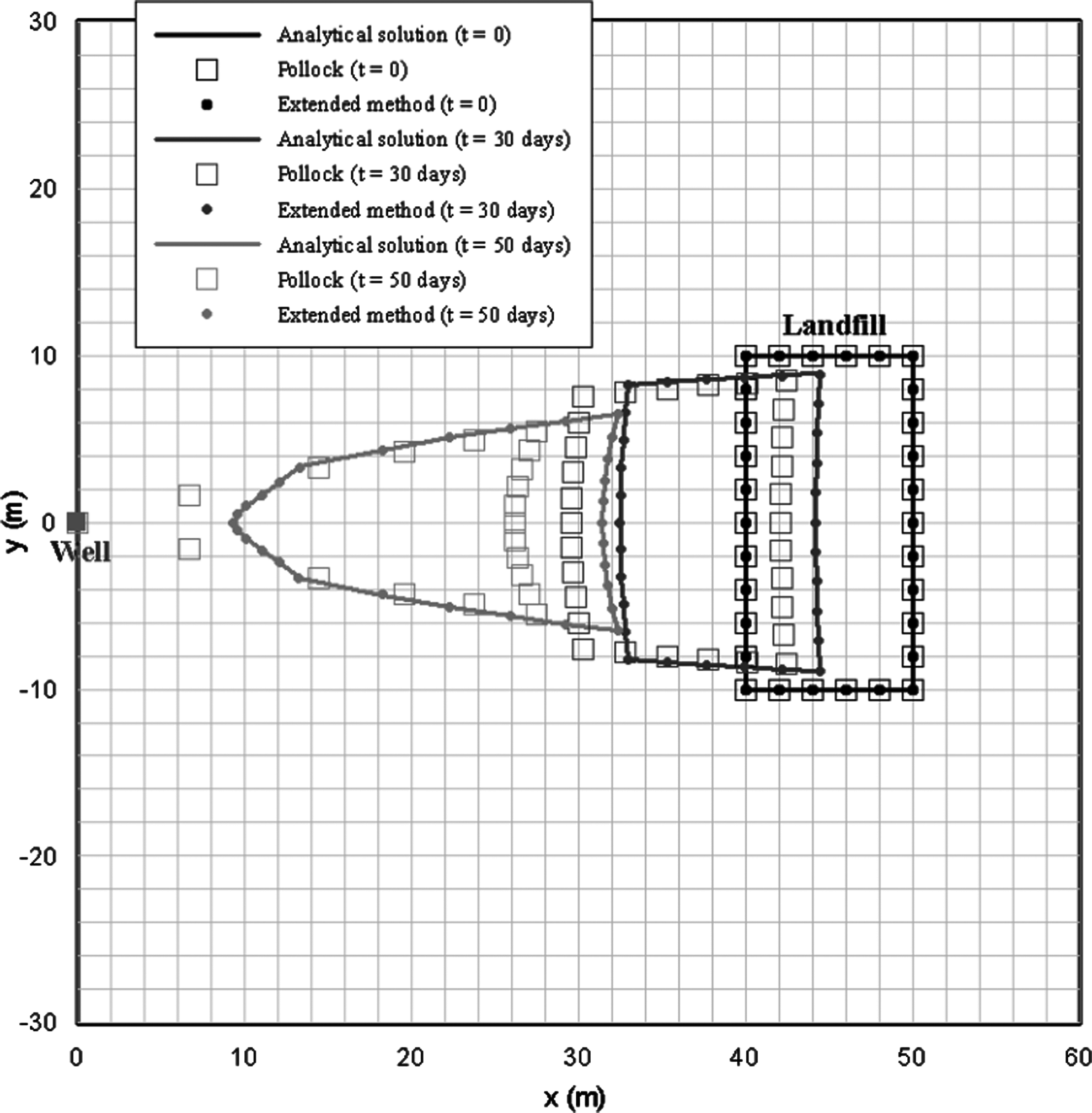Here, Q_P(t) was set to \documentclass{aastex} \usepackage{amsbsy} \usepackage{amsfonts} \usepackage{amssymb} \usepackage{bm} \usepackage{mathrsfs} \usepackage{pifont} \usepackage{stmaryrd} \usepackage{textcomp} \usepackage{portland, xspace} \usepackage{amsmath, amsxtra} \pagestyle{empty} \DeclareMathSizes {10} {9} {7} {6} \begin{document} \begin{align*}Q_P ( t ) = 3.8 t \ [ { \rm m}^3 / { \rm day} ] \tag{7}\end{align*}\end{document}

FIG. 2.

Results of Pollock's method and Suk's method with the analytical solution.

If the pumping well is operated according to the schedule above, the velocity field can be written as follows: \documentclass{aastex} \usepackage{amsbsy} \usepackage{amsfonts} \usepackage{amssymb} \usepackage{bm} \usepackage{mathrsfs} \usepackage{pifont} \usepackage{stmaryrd} \usepackage{textcomp} \usepackage{portland, xspace} \usepackage{amsmath, amsxtra} \pagestyle{empty} \DeclareMathSizes {10} {9} {7} {6} \begin{document} \begin{align*}V_x ( x , y , t ) = - \frac { Q_P ( t ) } { 2 \pi \sqrt { x^2 + y^2 } } \times \frac {x} {\sqrt {x^2 + y^2}} \tag {8} \end{align*}\end{document} \documentclass{aastex} \usepackage{amsbsy} \usepackage{amsfonts} \usepackage{amssymb} \usepackage{bm} \usepackage{mathrsfs} \usepackage{pifont} \usepackage{stmaryrd} \usepackage{textcomp} \usepackage{portland, xspace} \usepackage{amsmath, amsxtra} \pagestyle{empty} \DeclareMathSizes {10} {9} {7} {6} \begin{document} \begin{align*}V_y ( x , y , t ) = - \frac { Q_P ( t ) } { 2 \pi \sqrt { x^2 + y^2 } } \times \frac { y } { \sqrt { x^2 + y^2 } } \tag {9}\end{align*}\end{document}

Since the velocity field is directed toward the pumping well, a leachate plume in the landfill will migrate to the pumping well. To track the plume, the particle tracking method was performed using Suk's method and Pollock's method. The results of Suk's method were then compared with those of Pollock's method and demonstrated that Suk's method produces a better match to the exact solution than Pollock's method. Because the velocity field varies according to the location and time, the shape of the plume changed with time, even though dispersion, sorption, decay or growth, and any transformation were not considered. This suggests that the relative distance between the two particles within the plume will change with time as the plume evolves.

Modified random-walk particle tracking using Suk's particle tracking method

The efficiency and accuracy of Suk's method in the framework of random-walk particle tracking (RWPT) was evaluated to illustrate the practical applicability of Suk's method to RWPT. RWPT can be seen as an extension of the advective particle tracking approach (Bensabat et al., 2000; Pollock, 1988; Suk and Yeh, 2009). In contrast to advective particle tracking approaches, in RWPT, dispersive effects are considered. RWPT has been used successfully to simulate conservative and reactive transport in porous media (Ahlstrom et al., 1977; Prickett et al., 1981; Uffink, 1985; Tompson et al., 1987; Tompson, 1993). This method is computationally appealing, because it is grid independent and therefore, given the proper conditions, will require little computer storage compared to FEM, FDM, and the method of the characteristic model. In addition, RWPT does not suffer from numerical dispersion in problems dominated by advection. The traditional FEM and FDM generally perform poorly under such conditions unless the computational grid is highly resolved. As a result, RWPT has been developed to be used primarily when the advection-dispersion equation is strongly advection dominated. Despite these advantages, RWPT has the shortcomings, of the roughness of the simulated distributions in space and time due to statistical fluctuations and resolution problems, even though its relative size can be decreased by increasing the number of particles used (Kinzelbach, 1988). Furthermore, when a discontinuity in the velocity or effective porosity yields a discontinuous dispersion tensor, a local solute mass conservation problem occurs (LaBolle et al., 1996). The problem of local solute mass conservation has been widely discussed and a range of approaches have been suggested to overcome it (Hoteit et al, 2002; LaBolle et al., 1996, LaBolle et al., 1998, LaBolle et al., 2000; Uffink, 1985; Semra et al., 1993).

The standard FEM or FDM normally does not produce velocity derivable at the interface of two adjacent elements in a nonuniform flow. Hence, computing the dispersion coefficient derivatives for RWPT using either FEM or FDM will yield erroneous values (Hoteit et al., 2002, Park et al., 2008). Therefore, the discontinuous velocity will result in local mass conservation errors unless a correction is made. To prevent these errors, Park et al. (2008) used the global node-based velocity originally proposed by Yeh (1981) to resolve the discontinuities of flow velocity at the element or cell boundaries and to obtain a continuous velocity map over the model domain. Since the velocity is interpolated continuously over the model domain and the particle object knows the element index, the continuous velocity for the particle can be obtained along with the other subsequent properties, such as the dispersion tensor, derivative of velocity, and dispersion coefficient derivatives. Park et al. (2008) showed that their proposed RWPT method successfully reduced the number of particles by approximately two orders of magnitude without losing the accuracy of the concentration contours. In examples for this study, the local mass conservation problem was avoided by assuming analytically known velocity fields, obtaining global node-based velocities from the known velocity distribution by superposing a spatial discretization mesh on the computational region, and by using the inverse distance method as a velocity interpolation. Hence, the particle velocities at any location which particle tracks can be interpolated continuously over the model domain.

Implementation of the RWPT scheme included the advection movement of particles, based on the groundwater flow velocity, calculation of the gradient term in the dispersion tensor for a direct analogy of the Fokker-Plank equation with the solute transport equation, and a random movement of the particle superimposed to the movement with the groundwater flow velocity for a local scale dispersion. Within the knowledge of the author, almost all RWPT approaches have computed the advection movement of particles, using what we call a single velocity approach, that is, using only velocities at the old time level to compute the advection movement (Kinzelbach, 1986; LaBolle et al., 1996; Hassan et al., 1997; Hoteit et al., 2002; Tompson and Gelhar, 1990; Park et al., 2008). Although a single velocity approach does give a simple calculation because the velocities at the old time level are always known explicitly, it does not yield efficient results compared to other advanced advective particle tracking approaches (Cheng et al., 1996; Suk and Yeh, 2009, 2010; Bensabat et al., 2000). Accordingly, the present study modified the RWPT scheme to incorporate Suk's particle tracking method and to calculate efficient advective particle tracking. The result was compared with the original RWPT scheme, which used the single velocity approach.

RWPT scheme

Simulation of advective and diffusive mass transport using RWPT begins by solving the following stochastic differential equation (Kinzelbach, 1988) \documentclass{aastex} \usepackage{amsbsy} \usepackage{amsfonts} \usepackage{amssymb} \usepackage{bm} \usepackage{mathrsfs} \usepackage{pifont} \usepackage{stmaryrd} \usepackage{textcomp} \usepackage{portland, xspace} \usepackage{amsmath, amsxtra} \pagestyle{empty} \DeclareMathSizes {10} {9} {7} {6} \begin{document} \begin{align*} x_p (t + \Delta t) = x_p (t) + \left ( V_x ( x_p (t) , y_p (t) , t ) + \frac {\partial D_ {xx}} {\partial x} + \frac {\partial D_ {xy}} {\partial y} \right) \Delta t \\ + Z_1 \sqrt { 2 \alpha_L \mid V \mid \Delta t } \frac { V_x } { \mid V \mid } - Z_2 \sqrt { 2 \alpha_T \mid V \mid \Delta t } \frac { V_y } { \mid V \mid } \tag {10} \end{align*}\end{document} \documentclass{aastex} \usepackage{amsbsy} \usepackage{amsfonts} \usepackage{amssymb} \usepackage{bm} \usepackage{mathrsfs} \usepackage{pifont} \usepackage{stmaryrd} \usepackage{textcomp} \usepackage{portland, xspace} \usepackage{amsmath, amsxtra} \pagestyle{empty} \DeclareMathSizes {10} {9} {7} {6} \begin{document} \begin{align*} y_p ( t + \Delta t ) = y_p ( t ) + \left( V_y ( x_p ( t ) , y_p ( t ) , t ) + \frac {\partial D_ { yx }} {\partial x} + \frac {\partial D_ { yy }} {\partial y} \right) \Delta t \\ + Z_1 \sqrt { 2 \alpha_L \mid V \mid \Delta t } \frac {V_y} {\mid V \mid} + Z_2 \sqrt {2 \alpha_T \mid V \mid \Delta t} \frac {V_x} {\mid V \mid} \tag {11} \end{align*}\end{document}

with \documentclass{aastex} \usepackage{amsbsy} \usepackage{amsfonts} \usepackage{amssymb} \usepackage{bm} \usepackage{mathrsfs} \usepackage{pifont} \usepackage{stmaryrd} \usepackage{textcomp} \usepackage{portland, xspace} \usepackage{amsmath, amsxtra} \pagestyle{empty} \DeclareMathSizes {10} {9} {7} {6} \begin{document} \begin{align*}V_x = V_x ( x_p ( t ) , y_p ( t ) , t ) \tag {12}\end{align*}\end{document} \documentclass{aastex} \usepackage{amsbsy} \usepackage{amsfonts} \usepackage{amssymb} \usepackage{bm} \usepackage{mathrsfs} \usepackage{pifont} \usepackage{stmaryrd} \usepackage{textcomp} \usepackage{portland, xspace} \usepackage{amsmath, amsxtra} \pagestyle{empty} \DeclareMathSizes {10} {9} {7} {6} \begin{document} \begin{align*}V_y = V_y ( x_p ( t ) , y_p ( t ) , t ) \tag {13}\end{align*}\end{document} \documentclass{aastex} \usepackage{amsbsy} \usepackage{amsfonts} \usepackage{amssymb} \usepackage{bm} \usepackage{mathrsfs} \usepackage{pifont} \usepackage{stmaryrd} \usepackage{textcomp} \usepackage{portland, xspace} \usepackage{amsmath, amsxtra} \pagestyle{empty} \DeclareMathSizes {10} {9} {7} {6} \begin{document} \begin{align*}\mid V \mid = \sqrt{{V_x}^2 + {V_y}^2} \tag {14}\end{align*}\end{document}

where x_p(t) and y_p(t) are the coordinates of the particle location at time t, Δt is the time step, Z_i is the normally distributed random number with a zero mean and unit variance, and α_L and α_T are the longitudinal and transverse dispersivities, respectively. Here, D_ij is the hydrodynamic dispersion tensor (Bear, 1979), which is defined as follows: \documentclass{aastex} \usepackage{amsbsy} \usepackage{amsfonts} \usepackage{amssymb} \usepackage{bm} \usepackage{mathrsfs} \usepackage{pifont} \usepackage{stmaryrd} \usepackage{textcomp} \usepackage{portland, xspace} \usepackage{amsmath, amsxtra} \pagestyle{empty} \DeclareMathSizes {10} {9} {7} {6} \begin{document} \begin{align*}D_ { ij } = \alpha_T \mid V \mid \delta_ { ij } + ( \alpha_L - \alpha_T ) \frac { V_iV_j } { \mid V \mid } + D^d \tau_ { ij } \tag { 15 } \end{align*}\end{document}

where δ_ij is the Kronecker symbol, D^d is the molecular diffusion coefficient, and τ_ij is the tortuosity tensor. The spatial derivatives of the dispersion coefficient in Eqs. (10) and (11) can be expressed as a function of the derivatives of the velocity as Hoteit et al. (2002) have reported.

Performance analysis of the modified RWPT method under only temporally varying velocity fields

The only temporally varying velocity fields such that the advection velocities in the x-axis become larger as the simulation time passes are assumed as follows: \documentclass{aastex} \usepackage{amsbsy} \usepackage{amsfonts} \usepackage{amssymb} \usepackage{bm} \usepackage{mathrsfs} \usepackage{pifont} \usepackage{stmaryrd} \usepackage{textcomp} \usepackage{portland, xspace} \usepackage{amsmath, amsxtra} \pagestyle{empty} \DeclareMathSizes {10} {9} {7} {6} \begin{document} \begin{align*}V_x ( t ) = 1 + t^2 , V_y ( t ) = 0 \tag{16}\end{align*}\end{document}

It should be noted that the velocities are the same at all locations in a computational domain. In addition, it was assumed that α_L=α_T=1.0 m. The initial and boundary conditions are given by Eqs. (17) and (18), respectively. \documentclass{aastex} \usepackage{amsbsy} \usepackage{amsfonts} \usepackage{amssymb} \usepackage{bm} \usepackage{mathrsfs} \usepackage{pifont} \usepackage{stmaryrd} \usepackage{textcomp} \usepackage{portland, xspace} \usepackage{amsmath, amsxtra} \pagestyle{empty} \DeclareMathSizes {10} {9} {7} {6} \begin{document} \begin{align*} C & ( x , y , t ) \mid _{t = 0} \\ & = \begin{cases}1.0 g / m^3 \ 1900m \leq x \leq 2100 m , - 100 m \leq y \leq 100m \\ \quad0.0 \qquad \qquad \qquad \qquad\quad { \rm elsewhere}\end{cases} \tag {17}\end{align*}\end{document} \documentclass{aastex} \usepackage{amsbsy} \usepackage{amsfonts} \usepackage{amssymb} \usepackage{bm} \usepackage{mathrsfs} \usepackage{pifont} \usepackage{stmaryrd} \usepackage{textcomp} \usepackage{portland, xspace} \usepackage{amsmath, amsxtra} \pagestyle{empty} \DeclareMathSizes {10} {9} {7} {6} \begin{document} \begin{align*}C ( 0 , y , t ) = 0 , \ C ( 14000m , y , t ) = 0 , \\ C ( x , - 1000m , t ) = 0 , \ C ( x , 1000m , t ) = 0 \\0 \leq x \leq 14000m \ { \rm and} \ - 1000m \leq y \leq 1000 m \tag {18} \end{align*}\end{document}

where the porosity is 0.2 and the total injected mass of 8000 g is applied momentarily at t=0 in a rectangle area [1900 m, 2100 m]×[−100 m, 100 m] in such a way that the initial concentration within the rectangle area becomes 1.0 g/m³. In this example, enough particles (2 million) are used to avoid oscillation due to statistical fluctuations of RWPT. The total simulation time was 30 days.

Figures 3 and 4 show the numerical results of the modified RWPT, obtained using Suk's particle tracking method, and the original RWPT, obtained using the single velocity approach, at the times of interest (i.e., time=10, 20, 30 days) under various time steps. In this example, the modified RWPT always uses a time step size of 1 day. As shown in Figs. 3 and 4, as the time step size of single velocity approach is reduced from 1 day to 0.05 days, concentration distributions obtained by the single velocity approach become closer to those obtained by the modified RWPT with its time step size of 1 day. Therefore, the concentration distributions obtained by the single velocity approach with a time step size of 0.05 days are similar to those obtained by the modified RWPT with a time step size of 1 day. Considering the difference between the exact and computed locations of the plume peak, the difference calculated by the single velocity approach decreased with decreasing time step size, thus finally a single velocity approach with a time step size of 0.05 days achieves the same small difference as that with the modified RWPT using Suk's method with a time step size of 1 day (Table 1). This means that to achieve an accuracy similar to that of the modified RWPT, the original RWPT using single velocity approach requires time step sizes one twentieth that of the modified RWPT using Suk's method. Although the modified RWPT can adopt a time step size 20× larger than the original RWPT, it does not have 20× more computational advantage than the original RWPT, because Suk's particle tracking method is more computationally expensive than the single velocity approach. Therefore, as shown in Table 1, for the same level of accuracy, the modified RWPT using Suk's method has approximately 3.5× more computational efficiency than the original RWPT using the single velocity approach.

FIG. 3.

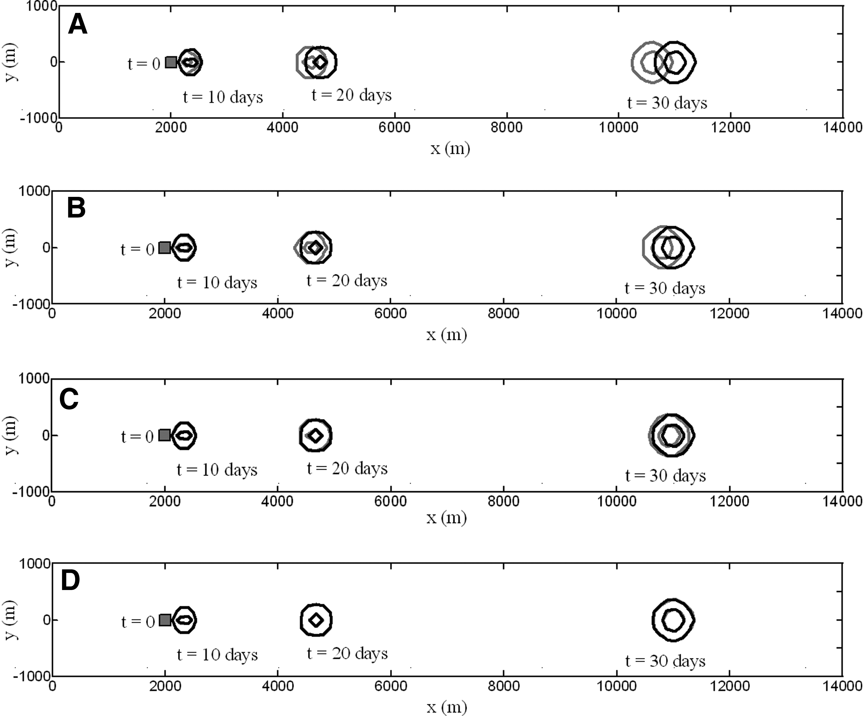
Concentration distributions obtained by the modified RWPT using Suk's particle tracking method (black lines) with fixed time step size of 1 day. and concentration distributions obtained by the original RWPT, using single velocity approach (gray lines) under various time step sizes. (a) 1 day, (b) 0.5 day, (c) 0.25 day, and (d) 0.05 day. The contour lines are shown for 0.02 g/m³ and 0.52 g/m³ at 10 days, for 0.02 g/m³ and 0.32 g/m³ at 20 days, and for 0.02 g/m³ and 0.12 g/m³ at 30 days.

FIG. 4.

Comparison of the concentration profiles on y=0 obtained by the modified RWPT using Suk's particle tracking method and the original RWPT using the single velocity approach under various time step sizes.

Table 1.

Comparison of CPU and Accuracy of Two Particle Tracking Methods Under Various Time Step Sizes

Model	CPU times (minutes)	Difference between exact and computed locations of peak divided by total transported distance (%)
RWPT (time step size=1 days)	6	4.9
RWPT (time step size=0.5 days)	12	2.5
RWPT (time step size=0.25 days)	24	1.2
RWPT (time step size=0.1 days)	61	0.5
RWPT (time step size=0.05 days)	122	0.3
RWPT using Suk's particle tracking method (time step size=1 days)	35	0.3

Performance analysis of the modified RWPT method under both temporally and spatially varying velocity fields

For the fourth example, velocity fields in which the groundwater flow converges from an injection well to an extraction well were established both temporally and spatially. The example has one injection well and one extraction well in an infinite isotropic confined aquifer. The injection well was located at (0, 0) with the pumping well located at (0, 200 m). The nodal velocities of the x and y components in steady-state flow can be expressed by Eqs. (19) and (20). \documentclass{aastex} \usepackage{amsbsy} \usepackage{amsfonts} \usepackage{amssymb} \usepackage{bm} \usepackage{mathrsfs} \usepackage{pifont} \usepackage{stmaryrd} \usepackage{textcomp} \usepackage{portland, xspace} \usepackage{amsmath, amsxtra} \pagestyle{empty} \DeclareMathSizes {10} {9} {7} {6} \begin{document} \begin{align*} V_x ( x , y ) = - \frac { 1 } { 2 \pi B \phi } \left( Q_1 { x - x_ \frac { w1 } { d_1 } ^2 } - Q_2 { x - x_ \frac { w2 } { d_2 } ^2 } \right) \tag {19} \end{align*}\end{document} \documentclass{aastex} \usepackage{amsbsy} \usepackage{amsfonts} \usepackage{amssymb} \usepackage{bm} \usepackage{mathrsfs} \usepackage{pifont} \usepackage{stmaryrd} \usepackage{textcomp} \usepackage{portland, xspace} \usepackage{amsmath, amsxtra} \pagestyle{empty} \DeclareMathSizes {10} {9} {7} {6} \begin{document} \begin{align*}V_y ( x , y ) = - \frac { 1 } { 2 \pi B \phi } \left( Q_1 { y - y_ \frac { w1 } { d_1 } ^2 } - Q_2 { y - y_ \frac { w2 } { d_2 } ^2 } \right) \tag {20}\end{align*}\end{document}

In this example, φ (porosity)=0.2, Q₁ (injection rate)=628 m³/day, Q₂ (extraction rate)=−628 m³/day , B (thickness of aquifer)=5 m, (x_w₁, y_w₁) and (x_w₂, y_w₂) are the coordinates of the injection and extraction wells, respectively, and \documentclass{aastex} \usepackage{amsbsy} \usepackage{amsfonts} \usepackage{amssymb} \usepackage{bm} \usepackage{mathrsfs} \usepackage{pifont} \usepackage{stmaryrd} \usepackage{textcomp} \usepackage{portland, xspace} \usepackage{amsmath, amsxtra} \pagestyle{empty} \DeclareMathSizes {10} {9} {7} {6} \begin{document} $$d_i = \sqrt{ ( x - x_{wi} ) ^2 + ( y - y_{wi} ) ^2}$$\end{document} . Bensabat et al. (2000) and Suk and Yeh (2009) adopted a plausible transient flow system by perturbing the steady-state velocities. The x components of the nodal velocities at the start and end times were set to 0.5× and 1.5× their counterparts under steady flow. The same velocity fields of Bensabat et al. (2000) and Suk and Yeh (2009) were employed to perform advection-dispersion simulation, using the modified RWPT and the original RWPT. In addition, it was assumed that α_L=α_T=0.01 m. The initial and boundary conditions are given by Eqs. (21) and (22), respectively. \documentclass{aastex} \usepackage{amsbsy} \usepackage{amsfonts} \usepackage{amssymb} \usepackage{bm} \usepackage{mathrsfs} \usepackage{pifont} \usepackage{stmaryrd} \usepackage{textcomp} \usepackage{portland, xspace} \usepackage{amsmath, amsxtra} \pagestyle{empty} \DeclareMathSizes {10} {9} {7} {6} \begin{document} \begin{align*} C ( x , y , t ) \mid _{t = 0} = \begin{cases}100.0 g / m^3 \ x = 0 , y = 20m \\ \quad0.0 \qquad \quad \; { \rm elsewhere}\end{cases} \tag {21}\end{align*}\end{document} \documentclass{aastex} \usepackage{amsbsy} \usepackage{amsfonts} \usepackage{amssymb} \usepackage{bm} \usepackage{mathrsfs} \usepackage{pifont} \usepackage{stmaryrd} \usepackage{textcomp} \usepackage{portland, xspace} \usepackage{amsmath, amsxtra} \pagestyle{empty} \DeclareMathSizes {10} {9} {7} {6} \begin{document} \begin{align*}C ( - 50m , y , t ) = 0 , \ C ( 200m , y , t ) = 0 , \\\ C ( x , 0 , t ) = 0 , C ( x , 200m , t ) = 0 \\ - 50m \leq x \leq 200 m \ { \rm and} \ 0 \leq y \leq 200m \tag {22} \end{align*}\end{document}

The fourth-order Runge–Kutta method with a very small time step size of 0.0001 day was used to obtain accurate solutions of the travel time and displacement of the plume peak only. According to the result of the fourth-order Runge–Kutta method, the particle departs at (0, 20 m) and arrives at (155.82 m, 127.65 m) after a simulation time of 237.3 days. This computed peak path line was used for a comparison with the concentration distributions obtained by the modified RWPT and the original RWPT. Because the fourth example assumes a more complicated flow system regarding both the magnitude and direction of the local velocity than the third example, more than 10 million particles were necessary to achieve a smoothness of the solution due to oscillations around the contours. As in the third example, as the time step size of the single velocity approach is reduced from 11.865 days to 0.2373 days in the fourth example, the concentration distributions obtained by the single velocity approach become similar to those determined by the modified RWPT with a time step size of 11.865 days (Fig. 5). In other words, plume distribution obtained by the single velocity approach with a large time step size of 11.865 days deviates greatly from the exact solution because, unlike Suk's method, the single velocity approach with a large time step size cannot perform accurate advective computation of the path line of the plume peak under such a rapidly changing, complicated flow system. On the other hand, since Suk's method with a large time step size of 11.865 days can provide a very accurate path line of the plume peak, the concentration contours at the times of interest obtained by the modified RWPT using Suk's method are well matched with those obtained by the original RWPT using the single velocity approach with much smaller time step of 0.2373 days (Fig. 5). Therefore, a time step size more than 50× larger than that of the original RWPT time step size can be used in the modified RWPT to achieve an accuracy of the concentration distribution similar to the original RWPT. On the other hand, as shown in Table 2, the modified RWPT has ∼4.3× more computational advantage regarding CPU time than the original RWPT because Suk's method is more computationally expensive for calculating a single advective step than the single velocity approach. Furthermore, as shown in Table 2, if strict comparisons between the modified RWPT and the original RWPT are performed regarding the difference between the exact and computed locations of the peak, the modified RWPT gives ∼43× more computational advantage in terms of CPU time than the original RWPT. This can be proved by noting that the even when the modified RWPT and original RWPT have time step sizes of 11.865 days and 0.02373 days, respectively, the differences between the exact and computed locations of the peak in Table 2 are similar.

FIG. 5.

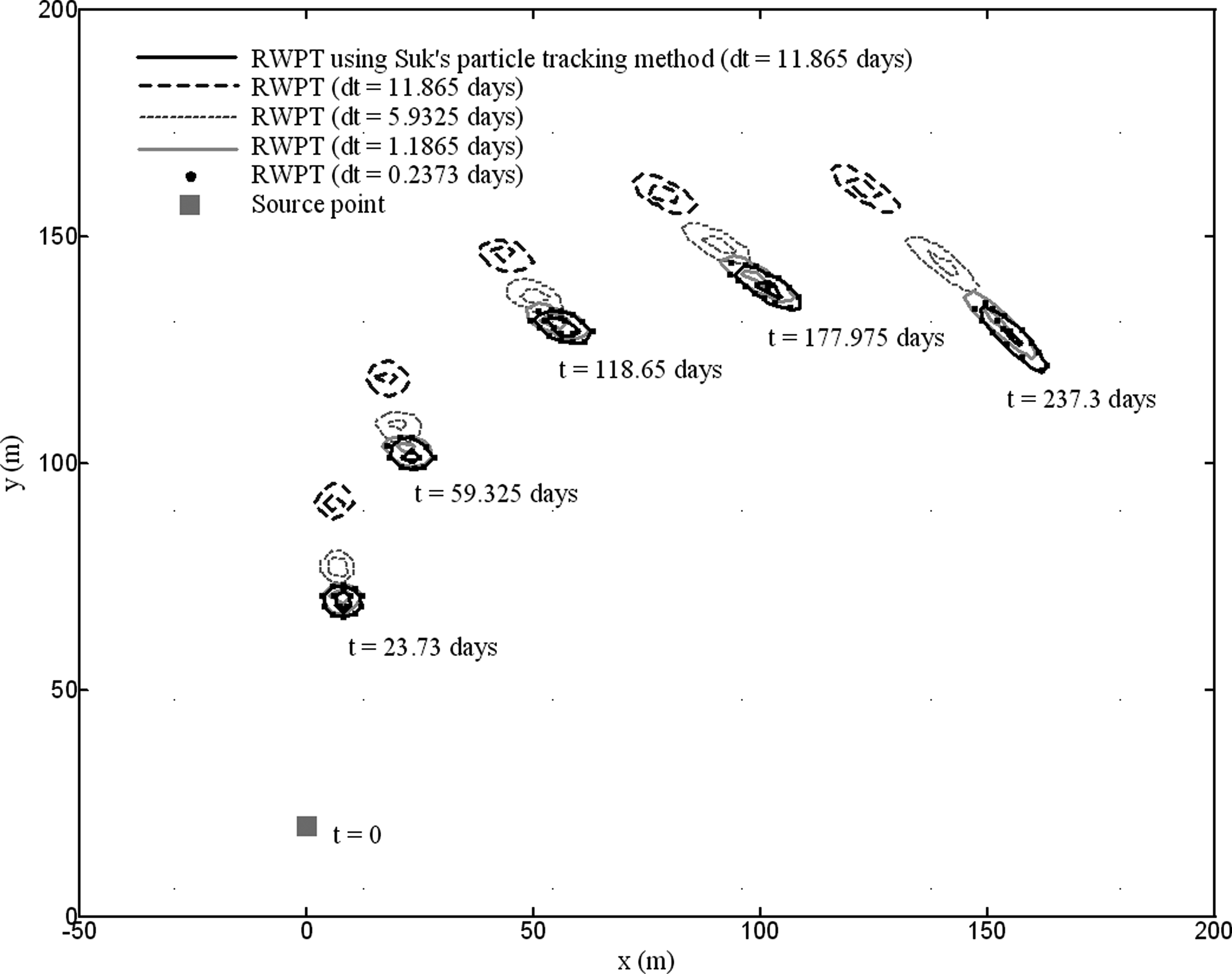
Comparison of the concentration distributions obtained by the modified RWPT using Suk's particle tracking method with a fixed time step size of 11.865 days and the original RWPT using the single velocity approach under various time steps under temporally and spatially varying velocity fields conditions. The contour lines are shown for 2 g/m³ and 12 g/m³ at 23.73 days; for 2 g/m³ and 12 g/m³ at 59.325 ays; for 2 g/m³ and 7 g/m³ at 118.65 days; for 2 g/m³ and 6 g/m³ at 177.975 days; and for 2 g/m³ and 5 /m³ at 237.3 days.

Table 2.

Comparison of CPU and Accuracy for Temporally and Spatially Varying Velocity Field Problems

Model	CPU times (minutes)	Difference between the exact and computed locations of peak divided by total transported distance (%)
RWPT (time step size=11.865 days)	21	20.0
RWPT (time step size=5.9325 days)	42	9.5
RWPT (time step size=2.373 days)	105	4.0
RWPT (time step size=1.1865 days)	210	2.1
RWPT (time step siz=0.59325 days)	420	1.1
RWPT (time step size=0.2373 days)	1,068	0.6
RWPT (time step size=0.02373 days)	10,735	0.2
RWPT using Suk's particle tracking method(time step size=11.865 days)	248	0.1

Conclusions and Discussion

An accurate and efficient particle tracking algorithm under complicated unsteady and steady flow conditions was developed by Suk and Yeh (2009, 2010). This particle tracking method was proposed, based on an element refinement that assumed that the velocity field was interpolated linearly in both time and space.

In this study, two examples (ASR and landfill leachate migration) were designed to illustrate the practical applicability of Suk's method to a real field of groundwater flow and transport, which have often been issues in geoscience. In the ASR example, the locations of the advancing front calculated using Suk's method were closer to the analytical solutions than those using Pollock's method (see Fig. 1). In the landfill leachate migration example, the performance of Suk's method was demonstrated through a comparison to Pollock's method (see Fig. 2) and showed that Suk's method provided a better match to the exact solution than Pollock's method. Although the performance of Suk's method was illustrated by considering only advection in the above two examples, it can be applied to the advective-dispersive transport problems in the same manner, because the advective-dispersive transport problem may be affected considerably by the particle tracking accuracy (Oliveira and Baptista, 1998). In other words, an inaccurate solution arising from Lagrangian step, including the particle tracking technique, may deteriorate the numerical solution obtained with either FEM or FDM for the dispersion process, because the advective-dispersive transport problem employs the operator splitting method, where the advective part is solved by the Lagrangian method first and the dispersive part is calculated using either FEM or FDM.

In addition, to illustrate the wide applicability of Suk's method to RWPT, the efficiency and accuracy of the method was evaluated in the framework of random-walk particle tracking (RWPT). The original RWPT was modified to incorporate Suk's method for efficient advection calculation. The concentration distributions obtained by the modified RWPT and the original RWPT were compared to confirm the superior performance of the modified RWPT over the original RWPT. In the case of the third example, assuming only a temporally varying velocity field, the modified RWPT, which used Suk's method, had ∼3.5× more computational efficiency than the original RWPT, which used the single velocity approach, as shown in Table 1. On the other hand, in the fourth example, assuming both temporally and spatially varying velocity fields, the modified RWPT had ∼43× more computational advantage in terms of CPU time than the original RWPT. Much more computational advantages regarding the CPU time occurred in the fourth example than the third example. This may be attributed to the complexity of the flow conditions. More computational advantages of the modified RWPT can be obtained under increasingly complex flow conditions. Thus under very complicated flow systems, Suk's method for advective computation may be more efficient in the framework of RWPT than a single velocity approach.

Footnotes

Acknowledgment

This study was supported by Korea Ministry of Environment as The GAIA Project (Grant no. 173-092-009).

Author Disclosure Statement

The author declares that no competing financial interests exist.

References

Ahlstrom

S.W.

, Foote

H.P.

, Arnett

R.C.

, Cole

C.R.

, Serne

R.J.

1977. Multi-component mass transport model: Theory and numerical implementation. Report BNWL-2127. Richland, WA: Battelle Pacific Northwest Laboratory.

Bensabat

, Zhou

, Bear

2000. An adaptive path line-based particle tracking algorithm for the Eulerian-Lagrangian method. Adv.Water Resour., 23:383.

Bear

1979. Hydraulics of Groundwater. New York: McGraw-Hill.

Bear

, Verruijt

1987. Modeling Groundwater Flow and Pollution: With Computer Programs for Sample Cases. Dordrecht: D. Reidel.

Brun

, Engesgaard

, Christensen

T.H.

, Rosbjerg

2002. Modelling of transport and biogeochemical processes in pollution plumes: Vejen landfill, Denmark. J. Hydrol., 256:228.

Cheng

H.P.

, Cheng

J.R.

, Yeh

G.T.

1996. A particle tracking technique for the Lagrangian Eulerian finite element method in multi-dimensions. Int. J. Numer. Meth. Eng., 39:1115.

Clement

T.P.

1997. RT3D (Version 1.0): A Modular Computer Code for Simulating Reactive Multispecies Transport in 3-Dimensional Groundwater Systems. A Report for the U.S. Department of Energy. Richland, WA: Battelle Pacific Northwest Laboratory, 59.

Diersch

H.J.G.

2006. FEFLOW 5.3, Finite Element Subsurface Flow & Transport Simulation System User's Manual. Berlin: WASY GmbH Institute for Water Resources Planning and Systems Research.

Harbaugh

A.W.

, Banta

E.R.

, Hill

M.C.

, McDonald

M.G.

2000. MODFLOW-2000, the U.S. Geological Survey Modular Ground-Water Model: User Guide to Modularization Concepts and the Ground-Water Flow Process. U.S. Geological Survey Open-File Report 00-92. Washington, DC: Department of the Interior.

10.

Hassan

A.E.

, Cushman

J.H.

, Delleur

J.W.

1997. Monte Carlo studies of flow and transport in fractal conductivity fields: Comparison with stochastic perturbation theory. Water Resour. Res., 33:2519.

11.

Hoteit

, Mose

, Younes

, Lehmann

, Ackerer

2002. Three-dimensional modeling of mass transfer in porous media using the mixed hybrid finite elements and the random-walk methods. Math.l Geo., 34:435.

12.

Javandel

, Doughty

L.C.

, Tsang

C.F.

1984. Groundwater Transport: Handbook of Mathematical Models. Water Resources Monograph Series, 10. Washington, DC: American Geophysical Union.

13.

Kinzelbach

1986. Groundwater Modeling: An Introduction with Sample Programs in BASIC. Netherlands: Elsevier Science Publishers B.V.

14.

Kinzelbach

1988. The random walk method in pollutant transport simulation. Custidio

et al. Groundwater Flow and Quality Modeling. Dordrecht: D. Reidel, 227.

15.

Konikow

L.F.

, Goode

D.J.

, Hornberger

G.Z.

1996. A Three-Dimensional Method-of-Characteristics Solute–Transport Model (MOC3D). U.S. Geological Survey Water Resources Investigation Report 96-4267. Reston, VA: U.S. Geological Survey.

16.

LaBolle

E.M.

, Fogg

G.E.

, Tompson

A.F.B.

1996. Random-walk simulation of transport in heterogeneous porous media: Local mass conservation problem and implementation methods. Water Resour. Res., 32:583.

17.

LaBolle

E.M.

, Quastel

, Fogg

G.E.

1998. Diffusion theory for transport in porous media: Transition probability densities of diffusion processes corresponding to advection–dispersion equations. Water Resour. Res., 34:1685.

18.

LaBolle

E.M.

, Quastel

, Fogg

G.E.

, Gravner

2000. Diffusion process in composite porous media and their numerical integration by random walks: Generalized stochastic differential equations with discontinuous coefficients. Water Resour. Res., 36:651.

19.

Lowry

C.S.

, Anderson

M.P.

2006. An assessment of aquifer storage recovery using ground water flow models. Ground Water, 44:661.

20.

Mackay

, Riley

M.S.

, Williams

G.M.

2001. Simulating groundwater contaminant migration at Villa Farm lagoons. Q. J. Eng. Geol. Hydroge., 34:215.

21.

Oliveira

, Baptista

A.M.

1998. On the role of tracking on Eulerian-Lagrangian solutions of the transport equation. Adv. Water Res., 21:539.

22.

Park

C.-H.

, Beyer

, Bauer

, Kolditz

2008. Using global node-based velocity in random walk particle tracking in variably saturated porous media: Application to contaminant leaching from road constructions. Environ. Geol., 55:1755.

23.

Pollock

D.W.

1988. Semianalytical computation of pathlines for finite-difference models. Ground Water, 26:743.

24.

Pollock

D.W.

1994. User's guide for MODPATH/MODPATH-PLOT, Version 3: A particle tracking post-processing package for MODFLOW. The U.S. Geological Survey finite-difference ground-water flow model. U.S. Geological Survey Open-File Report 94–464. Reston,VA: U.S. Geological Survey.

25.

Prickett

T.A.

, Naymik

T.G.

, Lonnquist

C.G.

1981. A “Random-Walk” Solute Transport Model for Selected Groundwater Quality Evaluations. Bulletin 65. Champaign, IL: State Water Survey Division.

26.

Schafer-Perini

A.L.

, Wilson

J.L.

1991. Efficient and accurate front tracking for two-dimensional groundwater flow models. Water Resour. Res., 27:1471.

27.

Semra

, Ackerer

, Mose

1993. Three-dimensional groundwater quality modeling in heterogeneous media. Wrobel

L.C.

, Brebbia

C.A.

Water Pollution II: Modeling, Measuring and Prediction. Southampton, United Kingdom: Wessex Institute of Technology Press, 3.

28.

Suk

, Yeh

G.T.

2009. Multidimensional Finite-Element particle tracking method for solving complex transient flow problems. J. Hydrol. Eng., 14:759.

29.

Suk

, Yeh

G.T.

2010. Development of particle tracking algorithms for various types of finite elements in multi-dimensions. Comput. Geosci. UK, 36:564.

30.

Tompson

A.F.B.

1993. Numerical simulation of chemical migration in physically and chemically heterogeneous porous media. Water Resour. Res., 29:3709.

31.

Tompson

A.F.B.

, Gelhar

L.W.

1990. Numerical simulation of solute transport in three-dimensional, randomly heterogeneous porous media. Water Resour. Res., 26:2541.

32.

Tompson

A.F.B.

, Vomvoris

E.G.

, Gelhar

L.W.

1987. Numerical simulation of solute transport in randomly heterogeneous porous media: Motivation, model development, and application. Report number UCID-21281. Livermore, CA: Lawrence Livermore National Laboratory.

33.

Uffink

G.J.M.

1985. A random walk method for the simulation of macrodispersion in a stratified aquifer. Dunn

F.X.

, Matthess

, Gras

R.A.

Relation of Groundwater Quality and Quantity. Oxfordshire, United Kingdom: IAHS Press, 103.

34.

Ward

J.D.

, Simmons

C.T.

, Dillon

P.J.

2008. Variable-density modeling of multiple-cycle aquifer storage and recovery (ASR): Importance of anisotropy and layered heterogeneity in brackish aquifers, J. Hydrol., 356:93.

35.

Yeh

G.T.

1981. On the computation of Darcian velocity and mass balance in the finite-element modeling of groundwater-flow. Water Resour. Res., 17:1529.

36.

Yeh

G.T.

, Sharp-Hansen

, Lester

, Strobl

, Scarbrough

1992. 3DFEMWATER/3DLEWASTE: Numerical Codes for Delineating Wellhead Protection Areas in Agricultural Regions Based on the Assimilative Capacity Criterion. Washington, DC: U.S. Environmental Protection Agency.

37.

Zheng

1990. MT3D User's Manual: A Modular Three-Dimensional Transport Model for Simulation of Advection, Dispersion, and Chemical Reactions of Contaminants in Groundwater Systems. Bethesda, MD: S.S. Papadopulos and Associates.