Predicting Total Organic Carbon Removal Efficiency and Coagulation Dosage Using Artificial Neural Networks

Abstract

Total organic carbon (TOC) in raw water is considered one of the major precursors to formation of disinfection by-products. Many drinking water treatment plants in the United States depend on coagulation, flocculation, and precipitation processes to bring treated water TOC levels to within acceptable limits. However, predicting TOC removal efficiency for a known coagulant dosage is not a trivial task and requires popular but time-consuming jar tests. This article presents successful implementation of artificial neural network (ANN) technology in predicting the TOC removal efficiency based on routinely measured physical and chemical raw-water characteristics and coagulant dosage. ANN predictions were better than multiple linear regression models. A new promising approach to develop a dose-response curve from the trained ANN is proposed and demonstrated in this study. This approach will facilitate instantaneous prediction of TOC at the outlet. It can also help in estimating optimal coagulant dosage in a drinking water treatment plant.

Introduction

Water treatment systems today use chlorine and other types of disinfectants to inactivate or kill microorganisms in drinking water. All chemical disinfectants (chlorine, monochloroamines, ozone, and chlorine dioxide) are known to form various types of disinfectant by-products (DBPs) when chemically reacted with DBP precursors present in the source water supply (Krasner, 1999).

The fact that long-term exposure to DBPs has been linked to several types of cancer resulted in the process of evaluating the regulatory approach for balancing the risks between disinfection of drinking water, residual chlorine, and the formation of DBPs (Zavaleta et al., 1999). After the discovery of trihalomethanes (THMs) in treated water, they were linked to increased cancer risk in the urinary and digestive tracts. Laboratory studies on animals have reported increased risk of bladder, colon, and rectal cancer as a result of long-term exposure to DBPs (USEPA, 2005a). Due to the exposure of large populations to chlorinated drinking water in the United States, conservative estimates of carcinogenic risk have been derived (Zavaleta et al., 1999). Subsequently, the maximum contaminant levels for total organic carbon (TOC) in source water and DBPs in the finished water have been set for federal and state regulatory purpose (USEPA, 2005a).

For the last decade, TOC has been one of the most important water quality parameters brought to the attention of the drinking water industry (USEPA, 1999). Today, many drinking water plants rely on coagulation, flocculation, and precipitation processes to remove TOC before disinfection (USEPA, 1998). In most cases, coagulation and softening remove nearly all the particulate precursor materials and a significant fraction of DOC precursors (USEPA, 1999). Under certain water quality conditions, TOC or DOC removal may be highly challenging. The regulatory changes under the Stage I Disinfectants and Disinfection Byproducts Rule ensure TOC removal to a considerable extent in the drinking water. If the TOC removal percentage can be increased by using an optimum coagulation dosage, then it would not only achieve desired turbidity removal, but also reduce the DBP formation in the distribution system. Therefore, the closer the operator is able to maintain the required TOC removal percentage, without over feeding the coagulant dose, the better the water quality supplied to the customers. Optimizing coagulant dose will also lower the operating, monitoring, and reporting cost to the utility (Gagnon et al., 1997).

Currently, most surface water treatment plants use the popular “jar test” (ASTM D 2035-08, 2008) to predict the optimum coagulant dosage to achieve desired turbidity reduction and TOC removal as required by state and federal regulations (Gagnon et al., 1997). When a jar test is used to predict the coagulant dosage to achieve required turbidity and TOC removal, the prediction may not be quick enough to make the changes to the process control, because raw water quality may vary with time. In addition, jar tests are normally performed only at limited times, often once a day, and, hence, any changes that occur during the rest of the day may not be reflected in the treatment process. Sometimes, jar tests may not predict the desired values accurately, because the prediction is based on a bench-scale testing procedure. Due to these reasons, it would be difficult to accurately replicate the chemical mixing, flocculation, and settling processes in the plant basins under different flow conditions. The interaction of various water quality parameters and TOC is very complex (Guzzella et al., 2004). Clark and Sivaganesan (2002) presented a mathematical model with two second-order terms for predicting the residual chlorine required to avoid pathogenic bacterial contamination in the treated water that can cause DBPs. Ossenbruggen et al. (1988) developed a linear regression model to predict THMs and several chlorination by-products by using raw water quality and control variables. Since the water quality varies from location to location, it is difficult to come up with a reliable mathematical model to predict TOC removal and required coagulant dosage.

An artificial neural network (ANN) is a data driven mathematical model that mimics the functioning of a human brain in learning and generalizing data. These models have been successfully used for pattern recognition, function approximation, and classification problems in different fields of engineering. Multi-layered feed-forward neural networks (Fig. 1) are the most commonly used form of ANNs in many environmental and water quality modeling studies.

FIG. 1.

Multi-layered feed-forward neural network model.

Maier and Dandy (2000) presented a review on the modeling issues related to ANN applications in water resources problems. They also discussed the importance of selecting proper input variables for efficient use of neural network models. Brion et al. (2002) used a neural-network-based classification scheme for sorting sources and ages of fecal contamination in water. Leeuwen et al. (1998) used an ANN model to assess the relationship between DOC and alum dosage found from jar testing for predicting the chemical requirements for drinking water treatment plants. Wen and Lee (1998) proposed a neural network based on multi-objective optimization scheme for water quality management. Fox et al. (2009) used an ANN for identifying the origin of sediments by using carbon isotopes. They also outlined the steps that should be followed in the development of such models. A task committee report from ASCE (2001a, 2001b) presented several successful applications of ANNs in water supply engineering. Collection and preprocessing of data, training, validation, cross training, and designing the ANN architecture were discussed in detail in this report.

In the past, many research applications used ANNs for modeling drinking water treatment process. Baxter et al. (2000) presented a guide in developing ANN processes models for finding the inter-relationship between drinking water treatment process inputs and outputs. Kulkarni and Chellam (2010) developed ANN models for predicting DBP formation during the drinking water treatment process by using the information collection rule treatment studies database. Baxter et al. (2000) presented the details of an ANN model that was developed for optimizing the removal of natural organic matter at the Rossdale Water Treatment Plant in Alberta, Canada. The ANN model developed in that study was used for enhancing coagulation by using multiple process parameters. Gontarski et al. (2000) used back-propagation ANN models to predict the output stream properties from a waste water treatment plant. In that study, TOC at the output stream was predicted by using inputs such as pH, TOC, pH in reactor, solid concentration, liquid flow rate of inlet stream, and recycled sludge flow rate. Shetty and Chellam (2003) used an ANN model for predicting membrane fouling during nanofiltration of ground and surface water by using commonly monitored water quality parameters. Shetty et al. (2003) developed an ANN model for predicting steady-state contaminant removal during nanofiltration of ground and surface water. In that research, operating conditions of the plant and physical properties were used as the input to the ANN model with the Levenberg-Marquardt training algorithm. Bowen et al. (1998a, 1998b) used an ANN model for predicting the filtration rate of colloids and proteins. These studies indicated the success of data-driven ANN models in water quality modeling.

This research examines the usefulness of an ANN for assessing TOC removal efficiency from raw water quality parameters and chemical dosages as inputs. In regular modeling applications, available data are divided into training, testing, and validation sets. For training and testing, 80% of the data are commonly used, whereas the remaining 20% are used for validation (Lingireddy and Brion, 2005). For example, with an available 80 data observations, 52, 12, and 16 data observations could be used for training, testing, and validation sets, respectively. Since the number of data observations available was small, cross-validation-based training strategy was adopted in this work as recommended by Neelakantan et al. (2002) instead of the conventional modeling.

Usually, developed ANN models are validated by using data that have not been used for training or testing. Training data are directly used for model training, and testing data are indirectly used, as their mean square error (MSE) is monitored during training (ASCE, 2001a). The third set (validation set) is used to evaluate the model performance on observations that the model has never seen. While applying the cross validation approach, this type of data split is not possible. Hence, relative strength effect (RSE)–based training termination was attempted in this study. When small datasets were available for developing the ANN model, Chandramouli et al. (2007) introduced an RSE–based optimal training termination strategy. They proposed using a dummy variable as an input to the model along with other inputs. The dummy variable is generated by using a random number generator. Since the dummy input is not a contributor to the output variable, it should have an RSE value close to zero when the ANN model is optimally trained. During training, this dummy variable is monitored, instead of monitoring the MSE value of the testing dataset. When the dummy variable RSE value reaches zero, optimal termination is performed. If the ANN is trained beyond this point, then some importance to the dummy variable begins to be assigned. This situation indicates overtraining. When this training method is used, instead of dividing the available data into training, testing and validation sets, data can be split into training and validation sets only. Since the dataset available for this study is small, a cross-validation scheme was used for initial model building, and the results were compared by using an RSE–based optimal training termination.

In this work, a novel approach is described to develop a dose-response curve with a trained ANN model. Developed dose-response curves will help in optimizing the coagulant dosage for a desired TOC removal efficiency. This method is very suitable for application in online plant operations. If TOC and other chemical dosages can be predicted by using this approach at a given water treatment facility for a given source water supply, then it could effectively complement the results provided by the jar tests.

Materials and Methods

Data source

Raw and treated water data used in this study were collected from Kentucky Division of Water's Drinking Water Branch for two surface water treatment systems in Central Kentucky. Both systems were run by the Kentucky American Water Company. Both the facilities use certified drinking water laboratories recognized by the Kentucky Division of Water. Kentucky American Water Company treats raw water obtained from Kentucky River at both drinking water plants in Lexington, Kentucky, for Lexington city water supply. Under Stage I Disinfectant and Disinfection Byproducts Rule, TOC data were available for these two public water systems from January 2002 to October 2003. In total, for the Lexington city supply, 80 data observations of 18 potential input parameters were available. Table 1 lists the observed parameters and the ranges.

Table 1.

Input Data Considered for Artificial Neural Network Model

		Initial model		Correlation coefficient with TOC-CFE (from field data)	Final model	Ranges of the parameters
Sl. No	Input parameter		RSE			Minimum	Maximum
1.	Plant flow (gallons/min)	√	0.28	0.40	√	161	1407
2.	Raw water alkalinity (mg/L as CaCO₃)	√	0.25	0.68	√	37	101
3.	Raw water TOC (mg/L)	√	0.95	0.54	√	1.2	5.2
4.	Coagulant: polymer PACL (mg/L)	√	−0.32	−0.19	√	0	213.8
5.	Coagulant: polymer cationic (mg/L)	√	0.45	0.42	√	0	5.2
6.	Coagulant: polymer aid (mg/L)	√	0.01	−0.21		0	1.9
7.	Disinfectant: chlorine (mg/L)	√	−0.15	0.47	√	4.5	11
8.	Raw water (pH)	√	−0.16	0.35	√	7	8
9.	Raw water hardness (total) (mg/L)	√	−0.49	0.58	√	74	268
10.	Raw water turbidity (NTU)	√	−0.52	−0.24	√	4	307
11.	Raw water fluorides (mg/L)	√	0.01	0.50		0	0.2
12.	Raw water iron (mg/L)	√	0.46	−0.20	√	0.01	5.5
13.	Raw water hardness (calcium) (mg/L)	√	0.68	0.59	√	50	144
14.	Raw water temperature (°F)	√	−0.22	0.68	√	38	90.2
15.	Polymer FeCl₂ (mg/L)	√	0.01	−0.19		0	57.9
16.	Flow at lock 10 (ft³/s)	√	−0.22	−0.34	√	192	35,200
17.	pH adjustment (mg/L)	√	−0.21	−0.30	√	0	34.6
18.	Disinfectant, pre ammonia (mg/L)	√	−0.06	−0.18		0	2.6

TOC, total organic carbon; RSE, relative strength effect; PACL, polymeric inorganic coagulant; CFE, combined filter effluent.

Artificial neural network

An ANN model consists of processing units called neurons arranged in layers. Neurons are inter-connected through weights. ANN models are trained by using historical data, and the knowledge acquired is stored in the inter-connecting weights (Maier and Dandy, 2001). These models learn by re-adjusting the weights of the connecting elements. A more detailed discussion on ANN learning may be found in Masters (1994) and ASCE (2001a, 2001b). First-order training algorithms (e.g., error back propagation training) and second-order training algorithms (e.g., conjugate gradient algorithm) have been successfully used in many research applications (Neelakantan et al., 2002). In the complex multi-dimensional space, most of the training algorithms attempt at minimizing the MSE by re-adjusting the weights. This study employed the Neurosort program Version II, developed by the faculty of Civil Engineering Department, University of Kentucky (Neurosort Version II, 2004).

ANN model development using cross-validation method

The water quality parameters and treatment data listed in Table 1 were considered for developing the ANN model. TOC at the combined filter effluent (here after referred to as TOC-CFE) is defined as the only output parameter to the ANN model. Correlation of each potential input to that of the TOC-CFE is given in Table 1.

All of the available 80 data observations were randomly shuffled to avoid seasonality effects before using them for ANN training. The available data observations were split into four groups. Cross validation was carried out by using those groups. To check the validity of the model, three batches (60 data) were used for model training, and one remaining batch (20 data) was used for the testing. In this manner, four different models were generated with three batches of data for training and the remaining one batch for testing. All four models used the same network architecture. In ANN modeling, proper input variable selection is an important task. Input parameters with a simple correlation coefficient >0.15 (to TOC-CFE) were selected for the preliminary ANN model. The input parameters for the final model were selected based on the RSE of each of the original inputs (Kim et al., 2001). Chandramouli et al. (2008) have successfully used the RSE–based approach for predicting enteric virus presence in river water used as a drinking water source. The inputs that have RSE values close to zero (Table 1) in the preliminary model were not considered in the final ANN model. In fact, 14 input variables considered for the final ANN model are also denoted in Table 1. The number of hidden layer neurons and the back propagation training parameters were decided after several experimental optimization runs.

The general rule of thumb in deciding the number of hidden layer neurons to include in an ANN model is to limit the number of inter-connecting weights to be less than the number of datasets used (Masters, 1994). Since this work involves a small dataset for modeling, this rule is violated even with only 3 hidden layer neurons and 14 inputs. Basheer and Hajmeer (2000) indicated that exotic problems such as those with high nonlinearity and hysteresis (Basheer, 2000) usually force the modeler to try networks with hidden layers that may not conform to the rule of thumb. Early training termination procedure helps in avoiding the overtraining (Masters, 1994). For setting up the best models, several trials were used. During these initial trial models, the indices, namely MSE, mean relative error (MRE), and coefficient of determination (r²) were monitored. Trials were started with two neurons in the hidden layer, and they were increased in steps to identify the best possible model that gave the best indices with an optimal network size. Table 2 shows the characteristics of the final ANN model. MSE and MRE were defined as \documentclass{aastex}\usepackage{amsbsy}\usepackage{amsfonts}\usepackage{amssymb}\usepackage{bm}\usepackage{mathrsfs}\usepackage{pifont}\usepackage{stmaryrd}\usepackage{textcomp}\usepackage{portland, xspace}\usepackage{amsmath, amsxtra}\pagestyle{empty}\DeclareMathSizes{10}{9}{7}{6}\begin{document} \begin{align*} {\rm MSE} = \frac {1} {pq} \sum_q \sum_{j = 1}^p \Big({y^t}_j - y_j \Big)^2 \tag{1} \end{align*} \end{document} \documentclass{aastex}\usepackage{amsbsy}\usepackage{amsfonts}\usepackage{amssymb}\usepackage{bm}\usepackage{mathrsfs}\usepackage{pifont}\usepackage{stmaryrd}\usepackage{textcomp}\usepackage{portland, xspace}\usepackage{amsmath, amsxtra}\pagestyle{empty}\DeclareMathSizes{10}{9}{7}{6}\begin{document} \begin{align*} {\rm MRE} = \frac {1} {pq} \sum_q \sum_{j = 1}^p \left| \, \frac {{y^t}_j - y_j} {{y^t}_j} \right| \times 100 \tag{2} \end{align*} \end{document}

Table 2.

Artificial Neural Network Model Training Parameters

Description	Value/number
No. of data	60
No. of inputs	14
No. of outputs	1
No. of neurons in the hidden Layer	8
Learning rate^a	0.1
Momentum factor^b	0.4
Bias term^c	0.3
Activation function in hidden layer	Sigmoidal
Activation function in output layer	Sigmoidal
Normalization adopted for each co-variant	Normalized by 1.2 times the maximum value in each co-variant domain

Learning rate is defined as the step size used by Artificial Neural Network training algorithm (Masters, 1993).

Momentum factor is a fraction that provides a control over the details used from the previous training step (Masters, 1993).

Bias term is a fraction used to eliminate bias during a training process (Masters, 1993).

where q=number of nodes in the output layer, p=number of patterns used for training/testing, y_j^t=the target output pattern value, and y_j=output from neural network model. Statistically, R² is defined as \documentclass{aastex}\usepackage{amsbsy}\usepackage{amsfonts}\usepackage{amssymb}\usepackage{bm}\usepackage{mathrsfs}\usepackage{pifont}\usepackage{stmaryrd}\usepackage{textcomp}\usepackage{portland, xspace}\usepackage{amsmath, amsxtra}\pagestyle{empty}\DeclareMathSizes{10}{9}{7}{6}\begin{document} \begin{align*} R^2 = \frac {\sum\limits_{j = 1}^p (y_j - {\overline {y}})^2} {\sum\limits_{j = 1}^p (y^t_j - {\overline {y}})^2} \tag{3} \end{align*} \end{document}

Table 3 shows training and testing results from the best model after cross validation. Testing results were used to find the superior model. The ANN model gave low MSE values and good R² values in all four batches. Performance of the ANN model was measured by examining the predicted results within a 15% confidence level. More than 75% of the testing set predictions and >85% of training predictions were within 15% confidence levels (Table 3). While terminating the training based on optimal training termination, proper generalization is achieved (Fig. 2). More training may reduce the MSE of training set, but the model will suffer in generalization. However, the MSE of the trained dataset may be slightly higher during optimal training termination. This fact can be noticed from Table 3. For batch 2, the number of data points within a 15% confidence level is only 69, whereas batch 3 had 72 such data points. However, the MSE for batch 2 was better than batch 3 (Table 3). This is because a few extreme points performed very well in batch 2, thus resulting in lower MSE. Figure 3 presents the testing results for batch 4 with a 15% confidence level. In most cases, ANN prediction was within 15% of the actual values. A training R² value of 0.907 and a testing R² value of 0.825 are impressive considering the size of the data set used for training the ANN model. A multiple linear regression model was also developed with the same inputs and TOC-CFE as output. During the cross-validation procedure, for the first three batches, the ANN performed better than multiple linear regression (MLR) (Fig. 4). In those three sets, MSE showed >50% improvement. In batch 4, the ANN was slightly better. When the cross validation procedure is used, the final performance was decided based on all the batch results. For the first 3 batches, the ANN outperforms MLR. This indicates the fact that the MLR model is not sufficient enough and reliable for this dataset. It indicates that the inter-relationships between the inputs and output are not linear. The results from this study clearly show the potential of using an ANN for predicting TOC-CFE values based on other routinely measured parameters and the coagulant dosage.

FIG. 2.

Training and testing data set results for batch 4.

FIG. 3.

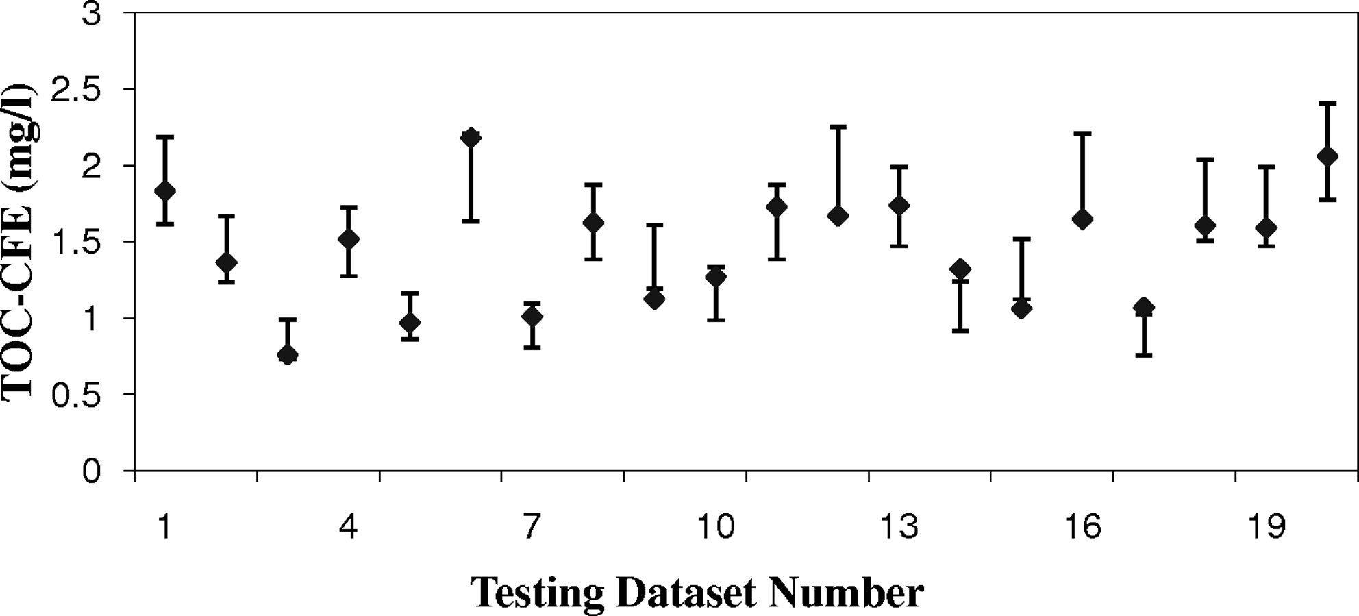
Testing set batch 4: ANN model performance with 15% confidence limit. ANN, artificial neural network.

FIG. 4.

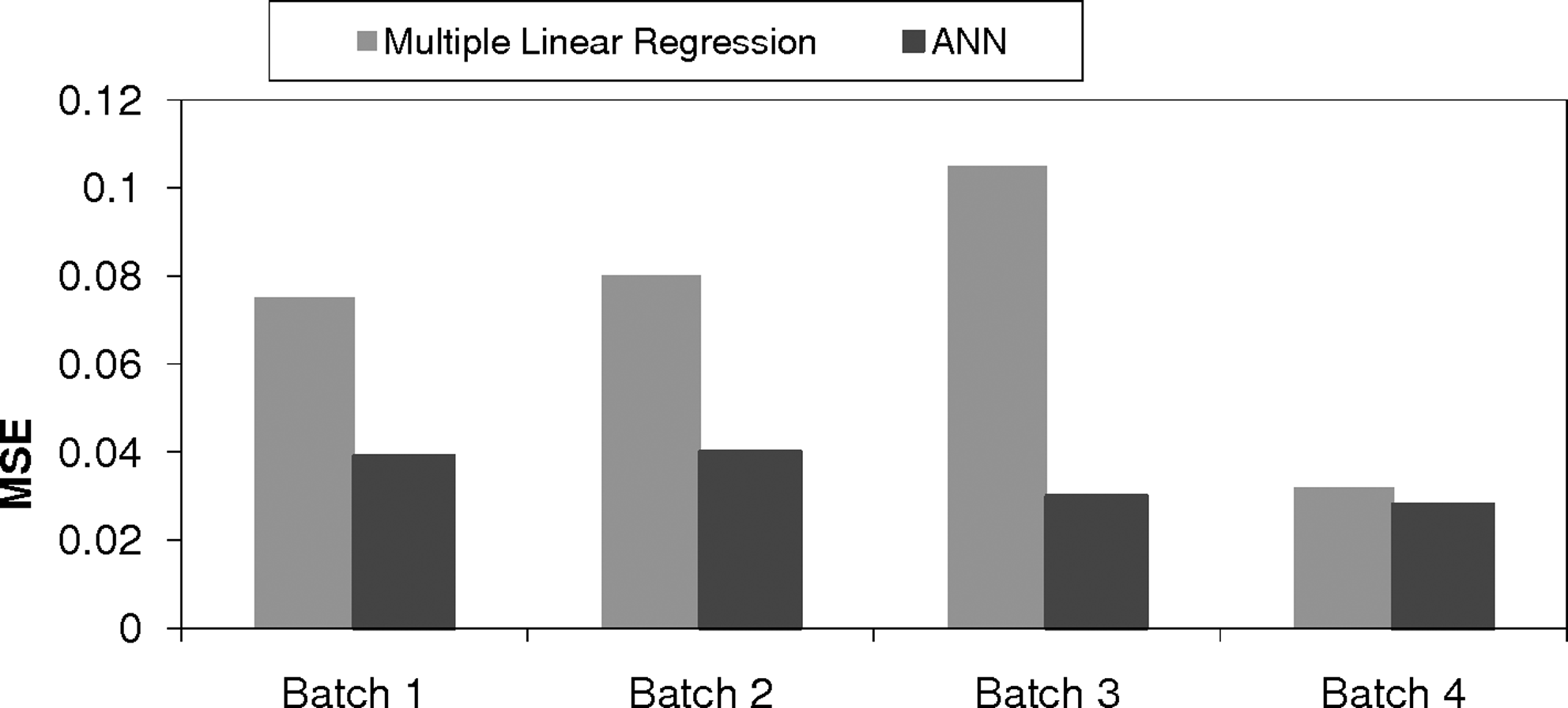
Comparing the performances of ANN and regression models in different batches by using testing results.

Table 3.

Training and Testing Results for Four Different Batches

	Training			Testing			No. of data points within 15% confidence level
Batch #	MRE	MSE	R²	MRE	MSE	R²	Training (out of 60)	Testing (out of 20)	Total
1	4.25	0.007	0.97	13.06	0.039	0.76	59	13	72
2	6.62	0.016	0.93	9.83	0.040	0.90	54	15	69
3	7.54	0.018	0.93	11.09	0.029	0.90	57	15	72
4	8.94	0.026	0.91	9.58	0.028	0.82	51	16	67

MSE, mean square error.

Validation of the ANN model using RSE–based optimal training termination

For validation, RSE–based optimal training termination was attempted. The initial model in this attempt has 19 input variables, which includes 18 inputs and 1 dummy variable. Overall, 60 data were used for the model training, and 20 data were used for the validation. The RSE of the dummy variable was monitored during the training. Training termination was performed when the RSE of the dummy variable reached zero. The advantage of this procedure is that unexposed data were used in the validation. While developing this model too, RSE values of other inputs were used for identifying inputs to the model. This model was also constructed in two stages. Stage I model results indicated the same four inputs for the elimination (Table 1). Stage II model was developed by eliminating the selected four inputs. The final model results were very similar to the cross-validation results (Fig. 5).

FIG. 5.

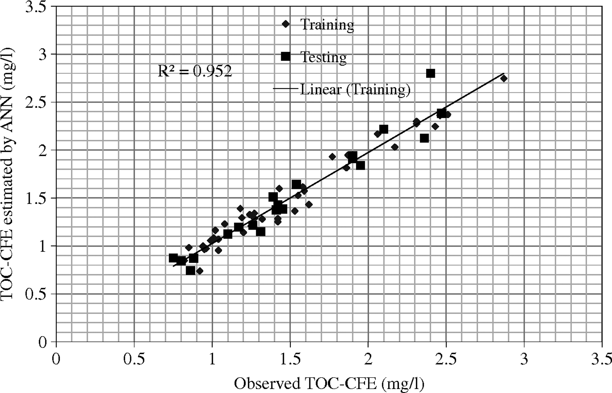
Training and validation data set results by using relative strength effect–based termination method.

Using trained ANN model for estimating coagulant dosage

The ANN model for estimating the TOC-CFE was successfully developed by using the 14 input parameters listed in Table 1. However, one could use a similar approach to develop an ANN that can predict the optimal coagulant dosage needed based on the raw-water characteristics and the specified TOC removal rate. This process requires developing a new ANN model and initial data processing. Subsequent efforts were made to use the initially trained ANN for estimating TOC-CEF to build a model that produces optimal coagulant dosage curves. The proposed scheme for using the developed ANN TOC-CEF model for online optimal coagulant dosage is presented in Fig. 6. Development of an optimal dosage curve can be accomplished in two ways. The first way is to draw a rule curve using a sensitivity analysis by considering an input variable (for this work, coagulant dosage). The second way is to re-write the ANN equation to have coagulant dose as an output, which is very complex. Based on an example from ASCE (2005), an expression for an ANN network with two inputs, one hidden layer and one output layer network (Fig. 7), is given in Equation (4):

FIG. 6.

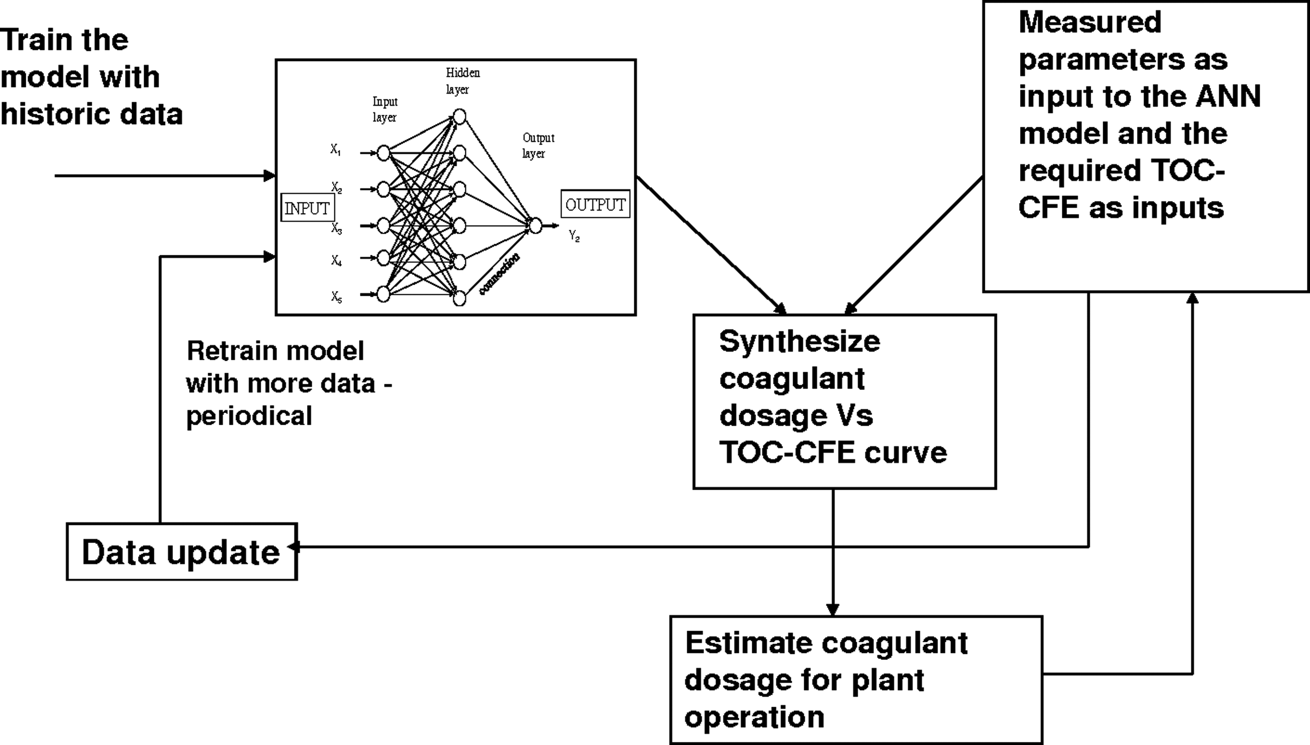
On-line monitoring using the ANN model for TOC-CFE. TOC, total organic carbon; CFE, combined filter effluent.

FIG. 7.

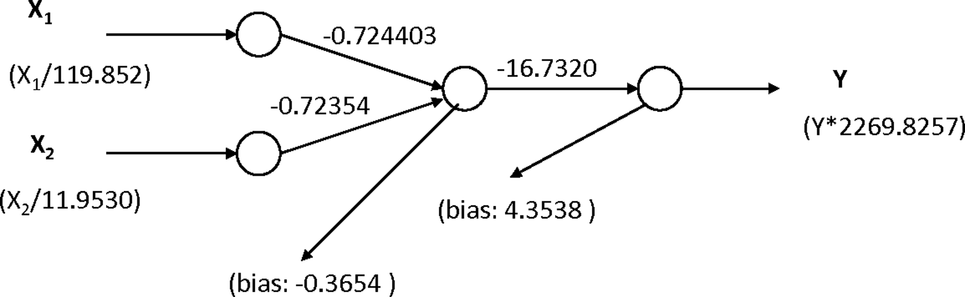
Trained ANN model with sigmoidal function.

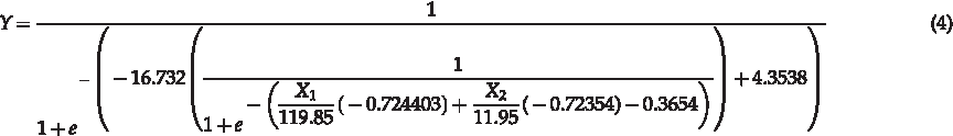
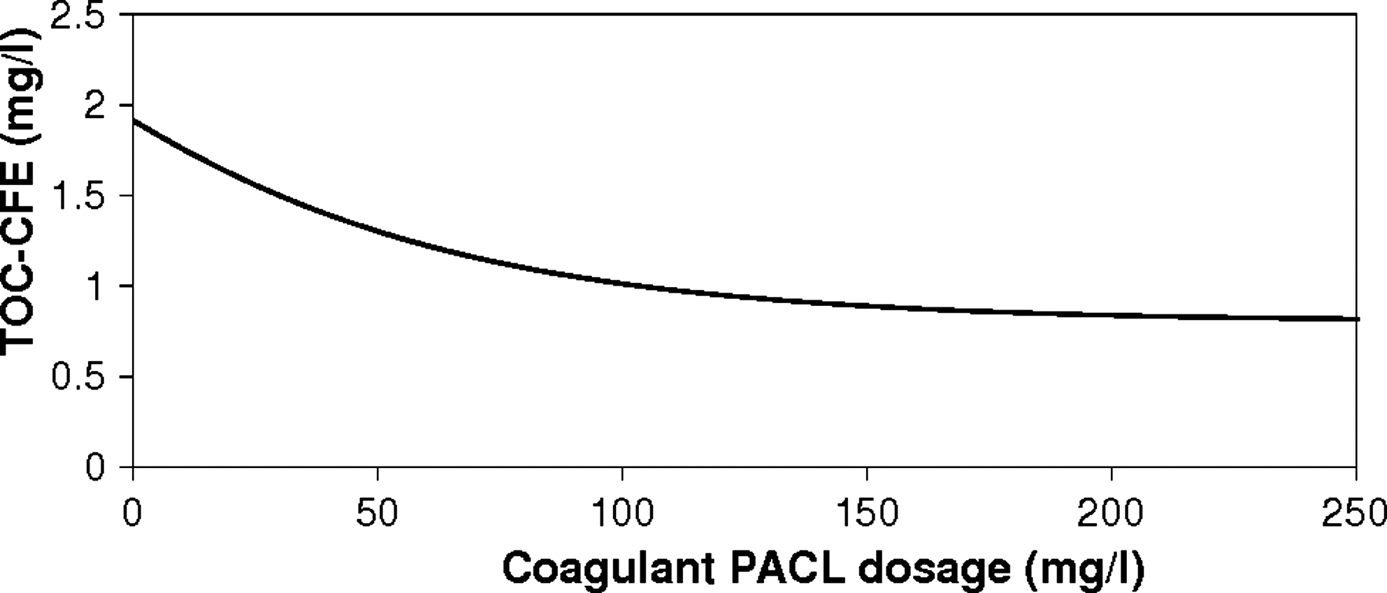
This equation can be re-arranged to \documentclass{aastex}\usepackage{amsbsy}\usepackage{amsfonts}\usepackage{amssymb}\usepackage{bm}\usepackage{mathrsfs}\usepackage{pifont}\usepackage{stmaryrd}\usepackage{textcomp}\usepackage{portland, xspace}\usepackage{amsmath, amsxtra}\pagestyle{empty}\DeclareMathSizes{10}{9}{7}{6}\begin{document} \begin{align*} \begin{split} X_2 = {11.95 \over - 0.72354} \Bigg[ - \ln {- 16.732 \over \ln \left[ {Y \over 1 - Y} \right] - 4.3538} + {X_1 (0.724403) \over 119.85} + 0.3654 \Bigg]\end{split} \tag{5} \end{align*} \end{document}

Using the re-arranged equation, X₂ can be estimated for a required Y and X₁. Utilizing this approach, by keeping the other 13 inputs the same, dosages were varied, and the resulting TOC-CFE outputs were estimated. Figure 8 shows one such dose-response graph developed for one of the sampled data observation. Using that graph, optimal dosage for the given initial conditions and the required TOC-CFE can be estimated. Figure 9 presents the set of rule graphs derived by varying the coagulant dosage as well as the raw water TOC for the same data point. Values of the raw water TOC were provided in the legend. For a given set of raw-water characteristics, one could develop a simplified dose-response rule curves by relating TOC-CFE as a function of coagulant dosage.

FIG. 8.

Coagulant dose estimation using ANN results.

FIG. 9.

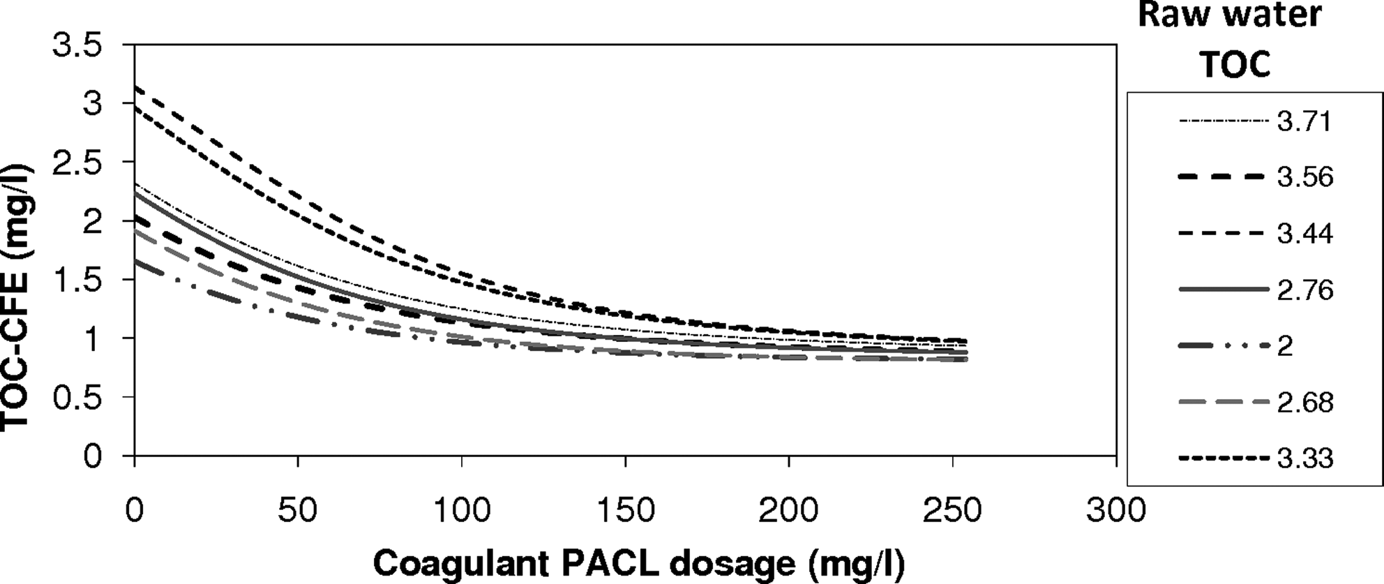
Coagulant dose estimation using ANN results for datasets with different initial values of raw water TOC.

This rule curve development requires an ANN model developed with all possible combinations of coagulant dosage. All four of the previously trained cross-validation models did not have enough data observations to cover the lower and upper bounds for coagulant dose needed for developing the full dose-response curve. Hence, instead of using one of the trained ANN models described in the previous sections, an ANN trained on a slightly different data set was used for developing the final dose-response curve. A similar curve could be developed for any coagulant used by the plant. For explaining this concept, polymeric inorganic coagulant (PACL) was used. Five artificial datasets were synthesized and added to the existing data by randomly selecting a data observation and setting its PACL value to zero and the corresponding TOC-CFE value to only 10% less than the raw-water TOC value. It was assumed that there would be some TOC removal through the filtration process even when no coagulant is added to the process. Although this is not an entirely accurate representation of reality, it helped in demonstrating the usefulness of the proposed ANN approach.

The dose-response curve produced along with the USEPA regulations (Table 4) could help the operator in choosing the right amount of coagulant dosage. Rule curves for several other combinations of different input parameters are also possible from the developed ANN model to study extreme influences to facilitate proper monitoring of the plant operation. Since the predictive efficiency of an ANN increases with larger sets of training data, one could periodically retrain the ANN, as more data are available by means of jar tests. The ANN model can further be strengthened by generating data in a controlled manner with different input parameter values fixed at different ranges between two extreme values. By doing so, the ANN model can acquire knowledge for all the domain ranges. In a plant operation, the trained ANN model could be used to find the TOC CFE instantly. By providing the other 13 observations as the inputs to the ANN model, the dose-response curve can be constructed and simultaneously used with the ANN model for controlling the coagulant dosage for the required TOC CFE value as indicated in Fig. 6.

Table 4.

Total Organic Carbon Removal Compliance Requirements

	Raw water alkalinity (mg/L as CaCO₃)
Raw TOC (mg/L)	0–60	>60–120	>120
≥2–4	35%	25%	15%
>4–8	45%	35%	25%
>8	50%	40%	30%

Conclusions

Conventional approaches for measuring the TOC removal efficiency employ the popular “jar tests.” The study reported in this article shows the potential for ANN technology for minimizing the dependency on jar tests for quicker and easier estimates for the treated water TOC values based on several routinely measured parameters. Although the case studies employed a relatively small database, the R² values between predicted and measured values of effluent TOC for training (0.91) and testing (0.83) models show the reliability of trained ANN models for the routine TOC removal efficiency calculations. The usefulness of the trained ANN was also demonstrated by the low MSE values for both training and testing samples. The ANN predictions were superior to conventional multiple linear regression model predictions. The article also shows the potential for developing a dose-response curve that can help the user to estimate the optimal coagulant dosage for a given set of raw-water quality parameters. The need for periodic re-training and cross-checking the validity of ANN predictions necessitates the use for conventional jar tests at a much reduced frequency and provides a quicker response to changing influent conditions.

Footnotes

Acknowledgment

C.V. acknowledges the support of startup funds provided by the Purdue University Calumet for conducting this research.

Author Disclosure Statement

No competing financial interests exist.

References

ASCE. 2001a. Task committee on artificial neural networks in hydrology, artificial neural networks in hydrology-I. Preliminary concepts. J. Hydrol. Eng. ASCE, 5:115.

ASCE. 2001b. Task committee on artificial neural networks in hydrology, artificial neural networks in hydrology-II, hydrologic applications. J. Hydrol. Eng. ASCE, 5:124.

ASTM D 2035-08. 2008. Standard Practice for Coagulation-Flocculation Jar Test of Water. West Conshohocken, PA: ASTM International.

Baxter

C.W.

, Stanley

S.J.

, Zhang

, Smith

D.W.

2000. Developing artificial neural network process models: a guide for drinking water utilities. Proceedings of 6th Environmental Engineering Specialty Conference of CSCE, London, Canada.

Basheer

2000. Selection of methodology for modeling hysteresis behavior of soils using neural networks. J. Comput. Aided Civ. Infrastruct. Eng., 5:445.

Basheer

, Hajmeer

2000. Artificial neural networks: fundamentals, computing, design, and application. J. Microbiol. Methods, 43:3.

Bowen

W.R.

, Jones

M.G.

, Yousef

H.N.S.

1998a. Dynamic ultrafiltration of proteins—a neural network approach. J. Membr. Sci., 146:225.

Bowen

W.R.

, Jones

M.G.

, Yousef

H.N.S.

1998b. Prediction of the rate of cross flow membrane ultrafiltration of colloids: a neural network approach. Chem. Eng. Sci., 53:3793.

Brion

G.M.

, Neelakantan

T.R.

, Lingireddy

2002. A neural network based classification scheme for sorting sources and ages of fecal contamination in water. Water Res., 36:3765.

10.

Chandramouli

, Lingireddy

, Brion

G.M.

2007. A robust training terminating criterion for back propagation ANNs applicable to small datasets. J. Comput. Civ. Eng. ASCE, 21:39.

11.

Chandramouli

, Neelakantan

T.R.

, Brion

G.M.

, Lingireddy

2008. Predicting enteric virus presence in surface waters using artificial neural networks. Environ. Eng. Sci., 25:62.

12.

Chowdhury

K.Z.

, Amy

G.L.

1999. Modeling disinfection by-product formation. Singer

. Formation and Control of Disinfection By-Products in Drinking Water. Denver, CO: AWWAChapter 353.

13.

Clark

R.M.

, Sivaganesan

2002. Predicting chlorine residuals in drinking water: second order model. J. Water Resour. Plann. Manage. ASCE, 128:152.

14.

Fox

J.F.

, Chandramouli

, Brion

G.M.

, Thompson

2009. Classification of erodible soils using artificial neural networks and biogeochemical indicators. Environ. Eng. Sci., 26:567.

15.

Gagnon

, Grandjean

B.P.A.

, Thibault

1997. Modeling of coagulant dosage in a water treatment plant. Artif. Intell. Eng., 11:401.

16.

Gontarski

C.A.

, Rodrigues

P.R.

, Mori

, Prenem

L.F.

2000. Simulation of an industrial wastewater treatment plant using artificial neural networks. Comput. Chem. Eng., 24:1719.

17.

Guzzella

, Monarca

, Zani

, Feretti

, Zerbini

, Buschini

, Poli

, Rossi

, Richardson

S.D.

2004. In vitro potential genotoxic effects of surface drinking water treated with chlorine and alternative disinfectants. Mut. Res., 564:179.

18.

Kim

C.Y.

, Bae

G.J.

, Hong

S.W.

, Park

C.H.

, Moon

H.K.

, Shin

H.S.

2001. Neural network based prediction of ground surface settlements due to tunneling. Comput. Geotech., 28:517.

19.

Krasner

W.S.

1999. Chemistry of disinfection by-products formation. Singer

. Formation and Control of Disinfection By-Products in Drinking Water. Denver, CO: AWWAChapter 224.

20.

Kulkarni

, Chellam

2010. Disinfection by-product formation following chlorination of drinking water: artificial neural network models and changes in speciation with treatment. Sci. Total Environ., 408:4202.

21.

Leeuwen

J.V.

, Bursill

, Chow

, Drikas

1998. Impact of Dissolved Organic Carbon on Water Treatment Process-Development of a Predictive Model for Process Optimization. Australian Water Quality Center.

22.

Lingireddy

, Brion

G.M.

2005. Artificial neural networks in water supply engineering. Reston, VA: Water Supply Engineering Committee, ASCE.

23.

Maier

H.R.

, Dandy

G.C.

2000. Neural networks for prediction of forecasting of water resources variables: a review of modeling issues and application. Environ. Model. Softw., 15:101.

24.

Maier

H.R.

, Dandy

G.C.

2001. Neural network based modeling of environmental variables: systematic approach. Math. Comput. Model., 33:669.

25.

Masters

1994. Practical Neural Network Recipes in C++ New York: Academic Press.

26.

Neelakantan

T.R.

, Lingireddy

, Brion

G.L.

2002. Effectiveness of different artificial neural network training algorithms in predicting protozoa risks in surface waters. J. Environ. Eng. ASCE, 128:533.

27.

Neurosort Version II, 2004. Department of Civil Engineering, University of Kentucky: Lexington, KY.

28.

Ossenbruggen

P.J.

, Gaudard

M.A.

, Collins

M.R.

1988. System model development with ill-conditioned data: case studies of trihalomethane formation in drinking water. Civ. Eng. Syst., 5:31.

29.

Shetty

G.R.

, Chellam

2003. Predicting fouling of nanofiltration membranes during municipal drinking water treatment using artificial neural networks. J. Membr Sci., 217:69.

30.

Shetty

G.R.

, Malki

, Chellam

2003. Predicting contaminant removal during municipal drinking water nanofiltration using artificial neural networks. J. Membr. Sci., 212:99.

31.

USEPA. 1998. National Primary Drinking Water Regulations: Intrerim Enhanced Surface Water Final Rule. Washington, DC: Environmental Protection Agency69478.

32.

USEPA. 1999. National Primary Drinking Water Regulations: Disinfectants and Disinfection By-Products Final Rule. Washington, DC: Environmental Protection Agency69390.

33.

Wen

C.G.

, Lee

C.S.

1998. A neural network approach to multi objective optimization for water quality management in a river basin. Water Resour. Res., 34:427.

34.

Zavaleta

O.J.

, Hauchman

F.S.

, Cox

M.W.

1999. Epidemiology and toxicology of disinfection by-products. Singer

P.C.

Formation and Control of Disinfection By-Products Drinking Water. Denver, CO: AWWAChapter 5424.