Linear and Nonlinear Modeling for Predicting Nickel Removal from Aqueous Solutions

Abstract

Mathematical models are widely used to predict removal rates of heavy metals from aqueous solutions. In this study, partial least squares (PLS), wavelet neural network (WNN), and support vector regression (SVR) were used to predict the amount of nickel (Ni) removal by dried sunflower stalks from a synthetic wastewater, based on experimental data sets from a laboratory batch mode. Effect of pH, initial concentration of the adsorbate, contact time, and dose of the adsorbent was considered in the adsorption process. Results showed that the coefficient of determination (R² or q²) for the relationship between the model-predicted and experimental data of the final concentration of Ni at calibration stage was 0.87, 0.98, and 0.99 and for cross-validation was 0.73, 0.8, and 0.91 for PLS, WNN, and SVR models, respectively. It was concluded that the SVR model performed relatively better than the other models due to its capability in capturing the nonlinear relationships between the variables. Grid search was a fast and effective method that optimized the hyperparameters in SVR modeling. The SVR and WNN models were also used to investigate the effect of different variables on Ni removal efficiency. The results showed that initial concentration of Ni and pH of the solution were more important in the adsorption process, relative to contact time and dose of the adsorbent.

Introduction

The surge of industrial activities has intensified environmental problems as seen, for example, in the accumulation of dangerous pollutants such as heavy metals (HMs) (Park et al., 2006). There has been increasing concern on the potential toxic effects of HM ions that make up the products and by-products of industries (Hansen et al., 2010).

Adsorption and biosorption are efficient methods that can be used for removal of HMs. Applying biotechnology in controlling and removing metal pollution is under much attention, and has gradually become a hot topic in the field of pollution control. Biosorption uses biomass to do the separation process (Basci et al., 2004; Zhang and Banks, 2006; Romera et al., 2008; Khambhaty et al., 2009; Bhatnagar and Sillanpaa, 2010).

Natural materials available in large quantities, or certain waste products from agricultural operations, may acquire potential as inexpensive adsorbents (Bhattacharya et al., 2006; Amarasinghe and Williams, 2007). Plant residues, which are mainly ligno-cellulosic materials, can inherently adsorb waste chemicals such as dyes and cations in water (Sun and Shi, 1998). One of the most effective adsorbents in this regard is sunflower stalks, which have a relatively large surface area that can provide intrinsic adsorptive cites for many adsorbates. The removal of metal ions such as copper, cadmium, zinc, and chromium ions from aqueous solutions has been studied using sunflower stalks as adsorbent (Sun and Shi, 1998; Benaissa and Elouchdi, 2007; Jain et al., 2009).

An attempt has been made in this article to study the adsorption behavior of dried sunflower biomass in aqueous solution containing Ni. The adsorption efficiency of a biosorbent can be evaluated quantitatively by a simple series of experiments including isotherms, kinetics (Zhang and Banks, 2006), and some computational methods. So, it is necessary to find some computational methods to correlate the removal efficiency of Ni(II) from wastewater with the process parameters.

There are a few researches in relation to modeling the removal efficiency of HMs through the biosorption process. The artificial neural network has been used successfully to predict the removal efficiency of some HMs from aqueous solutions (Prakash et al., 2008; Yetilmezsoy and Demirel, 2008; Sahinkaya, 2009). However, to the best of our knowledge, there is no report about using partial least squares (PLS), wavelet neural network (WNN), and support vector regression (SVR) to do this modeling.

The main objective of the present work was to test the PLS, WNN, and SVR models for prediction of Ni removal efficiency from wastewater by utilizing dried sunflower stalks as an economical bioadsorbent material.

Theory

Partial least squares

PLS is a multivariate statistical linear regression technique to extract the relationship between an array of output variables and an array of input variables. In this method, reduction in the dimensionality of the raw data is based on the input (X matrix) as well as the output data (Y matrix) and not just on the input data. Decomposition of X and Y is accomplished simultaneously as follows (Geladi and Kowalski, 1986): \documentclass{aastex} \usepackage{amsbsy} \usepackage{amsfonts} \usepackage{amssymb} \usepackage{bm} \usepackage{mathrsfs} \usepackage{pifont} \usepackage{stmaryrd} \usepackage{textcomp} \usepackage{portland, xspace} \usepackage{amsmath, amsxtra} \pagestyle{empty} \DeclareMathSizes {10} {9} {7} {6} \begin{document} \begin{align*}X = TP + DBT \tag{1}\end{align*}\end{document} \documentclass{aastex} \usepackage{amsbsy} \usepackage{amsfonts} \usepackage{amssymb} \usepackage{bm} \usepackage{mathrsfs} \usepackage{pifont} \usepackage{stmaryrd} \usepackage{textcomp} \usepackage{portland, xspace} \usepackage{amsmath, amsxtra} \pagestyle{empty} \DeclareMathSizes {10} {9} {7} {6} \begin{document} \begin{align*}Y = UQ + FBT \tag{2}\end{align*}\end{document}

where T and U are the X- and Y-block score matrices, P and Q are the X and Y loadings, and D and F are the residuals. PLS modeling contains the creation of relationship between projections of the dependent and independent variables (U and T, respectively), according to \documentclass{aastex} \usepackage{amsbsy} \usepackage{amsfonts} \usepackage{amssymb} \usepackage{bm} \usepackage{mathrsfs} \usepackage{pifont} \usepackage{stmaryrd} \usepackage{textcomp} \usepackage{portland, xspace} \usepackage{amsmath, amsxtra} \pagestyle{empty} \DeclareMathSizes {10} {9} {7} {6} \begin{document} \begin{align*}U = BT \tag{3}\end{align*}\end{document}

Wavelet neural network

Wavelet is a type of transformation that retains both time and frequency information of the signal (Zhong et al., 2001). In chemical studies, the time domain can be replaced by other domains such as wavelength. Wavelet transformation (WT) has versatile basis functions to be selected based on the type of the signal analyzed. In WT, all basis functions ψ_a,b(X) can be derived from a mother wavelet, ψ(x), through the following dilation and translation processes: \documentclass{aastex} \usepackage{amsbsy} \usepackage{amsfonts} \usepackage{amssymb} \usepackage{bm} \usepackage{mathrsfs} \usepackage{pifont} \usepackage{stmaryrd} \usepackage{textcomp} \usepackage{portland, xspace} \usepackage{amsmath, amsxtra} \pagestyle{empty} \DeclareMathSizes {10} {9} {7} {6} \begin{document} \begin{align*}\psi_ {a , b} ( X ) = a^ {- 1 / 2} \psi \bigg( \frac {x - b} {a} \bigg) \quad a , b \in R \ \rm and \ \it a > \rm 0 \tag {4} \end{align*}\end{document}

where the parameters of translation are \documentclass{aastex} \usepackage{amsbsy} \usepackage{amsfonts} \usepackage{amssymb} \usepackage{bm} \usepackage{mathrsfs} \usepackage{pifont} \usepackage{stmaryrd} \usepackage{textcomp} \usepackage{portland, xspace} \usepackage{amsmath, amsxtra} \pagestyle{empty} \DeclareMathSizes {10} {9} {7} {6} \begin{document} $$b \in R$$\end{document} and of dilation are \documentclass{aastex} \usepackage{amsbsy} \usepackage{amsfonts} \usepackage{amssymb} \usepackage{bm} \usepackage{mathrsfs} \usepackage{pifont} \usepackage{stmaryrd} \usepackage{textcomp} \usepackage{portland, xspace} \usepackage{amsmath, amsxtra} \pagestyle{empty} \DeclareMathSizes {10} {9} {7} {6} \begin{document} $$a \in R$$\end{document} and a >0 (R denotes real number). Mother wavelet, ψ(x), is a single, fixed function. Similar to the Morlet function, all basis functions are generated from the mother function. The continuous WT of a signal function such as f(x) is given by \documentclass{aastex} \usepackage{amsbsy} \usepackage{amsfonts} \usepackage{amssymb} \usepackage{bm} \usepackage{mathrsfs} \usepackage{pifont} \usepackage{stmaryrd} \usepackage{textcomp} \usepackage{portland, xspace} \usepackage{amsmath, amsxtra} \pagestyle{empty} \DeclareMathSizes {10} {9} {7} {6} \begin{document} \begin{align*}W ( a , b ) = \int \limits_0^{ \infty} \psi^* a , b ( x ) f ( x ) dx \tag{5}\end{align*}\end{document}

where the asterisk (*) represents the complex conjugate.

The WNN consists of three layers: input, hidden, and output. The calibration steps of WNN are described in Zhang et al. (2001). Briefly, the connections between input and hidden units and between hidden and output units are called weights, w_ti and W_t, respectively. The dilation and translation parameters, a_t and b_t, of the Morlet function for each node in the hidden layer are different, and they need to be optimized.

In WNN, the gradient descending algorithm is employed, and the error is minimized by adjusting W_t, w_ti, a_t, and b_t parameters. These parameters are adjusted using ΔW_t, Δw_ti, Δa_t, and Δb_t formulae as follows: \documentclass{aastex} \usepackage{amsbsy} \usepackage{amsfonts} \usepackage{amssymb} \usepackage{bm} \usepackage{mathrsfs} \usepackage{pifont} \usepackage{stmaryrd} \usepackage{textcomp} \usepackage{portland, xspace} \usepackage{amsmath, amsxtra} \pagestyle{empty} \DeclareMathSizes {10} {9} {7} {6} \begin{document} \begin{align*}\Delta W_t (\ j + 1 ) = - \eta \frac {\partial E} {\partial W_t (\ j )} + \alpha \ \Delta W_t (\ j ) \tag {6}\end{align*}\end{document} \documentclass{aastex} \usepackage{amsbsy} \usepackage{amsfonts} \usepackage{amssymb} \usepackage{bm} \usepackage{mathrsfs} \usepackage{pifont} \usepackage{stmaryrd} \usepackage{textcomp} \usepackage{portland, xspace} \usepackage{amsmath, amsxtra} \pagestyle{empty} \DeclareMathSizes {10} {9} {7} {6} \begin{document} \begin{align*}\Delta w_{ ti } (\ j + 1 ) = - \eta \frac {\partial E } { \partial w_ { t i } (\ j ) } + \alpha \ \Delta w_ { t \ i } (\ j ) \tag{7}\end{align*}\end{document} \documentclass{aastex} \usepackage{amsbsy} \usepackage{amsfonts} \usepackage{amssymb} \usepackage{bm} \usepackage{mathrsfs} \usepackage{pifont} \usepackage{stmaryrd} \usepackage{textcomp} \usepackage{portland, xspace} \usepackage{amsmath, amsxtra} \pagestyle{empty} \DeclareMathSizes {10} {9} {7} {6} \begin{document} \begin{align*}\Delta a_t (\ j + 1 ) = - \eta \frac {\partial E } { \partial a_t (\ j ) } + \alpha \ \Delta a_t (\ j ) \tag{8}\end{align*}\end{document} \documentclass{aastex} \usepackage{amsbsy} \usepackage{amsfonts} \usepackage{amssymb} \usepackage{bm} \usepackage{mathrsfs} \usepackage{pifont} \usepackage{stmaryrd} \usepackage{textcomp} \usepackage{portland, xspace} \usepackage{amsmath, amsxtra} \pagestyle{empty} \DeclareMathSizes {10} {9} {7} {6} \begin{document} \begin{align*}\Delta b_t (\ j + 1 ) = - \eta \frac { \partial E } { \partial b_t (\ j ) } + \alpha \ \Delta b_t (\ j ) \tag{9} \end{align*} \end{document}

where j is the number of iterations, and η and α are the learning rate and momentum term, respectively. The error function E is written as \documentclass{aastex} \usepackage{amsbsy} \usepackage{amsfonts} \usepackage{amssymb} \usepackage{bm} \usepackage{mathrsfs} \usepackage{pifont} \usepackage{stmaryrd} \usepackage{textcomp} \usepackage{portland, xspace} \usepackage{amsmath, amsxtra} \pagestyle{empty} \DeclareMathSizes {10} {9} {7} {6} \begin{document} \begin{align*}E = \frac { 1 } { 2 } \sum_ { n = 1 } ^N ( V_ { cn } - V_ { en } ) ^2 \tag { 10 } \end{align*}\end{document}

where V_cn and V_en are the calculated and experimental values, respectively, and N is the number of data for calibration.

Support vector machine

Support vector machine (SVM) was introduced by Vapnik (1998). For a given regression problem, the goal of SVM is to find the optimal hyperplane, from which the distance to all the data points is minimum (Smola and Scholkopf, 1998). Here, a basic comprehensive description of the concept underlying SVR modeling will be presented.

Consider a data set consisting of \documentclass{aastex} \usepackage{amsbsy} \usepackage{amsfonts} \usepackage{amssymb} \usepackage{bm} \usepackage{mathrsfs} \usepackage{pifont} \usepackage{stmaryrd} \usepackage{textcomp} \usepackage{portland, xspace} \usepackage{amsmath, amsxtra} \pagestyle{empty} \DeclareMathSizes {10} {9} {7} {6} \begin{document} $$G = ( x_i , y_i ) _{i = 1}^N$$\end{document} of N data points where each input x_i is mapped into the corresponding output y_i. Given that the data set realizes some unknown function g(x), we need to determine a function f that approximates g(x), based on the knowledge of the data set G. In SVM, x_i is first mapped into a higher dimensional space F via a nonlinear mapping, and linear regression is performed in this space. The SVM approximates the function as \documentclass{aastex} \usepackage{amsbsy} \usepackage{amsfonts} \usepackage{amssymb} \usepackage{bm} \usepackage{mathrsfs} \usepackage{pifont} \usepackage{stmaryrd} \usepackage{textcomp} \usepackage{portland, xspace} \usepackage{amsmath, amsxtra} \pagestyle{empty} \DeclareMathSizes {10} {9} {7} {6} \begin{document} \begin{align*}f ( x ) = \sum_{i = 1} \omega_i \varphi_i ( x ) + b \quad { \rm with} \quad \varphi : \Re^n \rightarrow F , \omega \in F \tag{11}\end{align*}\end{document}

where ω_i are the coefficients, and b is a threshold value. This approximation can be considered a hyperplane in the D-dimensional feature space F defined by the functions φ_i(x) where the dimensionality can be very high, possibly infinite. Since φ is fixed, ω_i can be determined from the data by minimizing the sum of empirical risk and a complexity term defined by \documentclass{aastex} \usepackage{amsbsy} \usepackage{amsfonts} \usepackage{amssymb} \usepackage{bm} \usepackage{mathrsfs} \usepackage{pifont} \usepackage{stmaryrd} \usepackage{textcomp} \usepackage{portland, xspace} \usepackage{amsmath, amsxtra} \pagestyle{empty} \DeclareMathSizes {10} {9} {7} {6} \begin{document} \begin{align*}R = \gamma \frac { 1 } { N } \sum_ { i = 1 } ^N | y_i - f ( x_i ) | _ { \varepsilon } + \frac { 1 } { 2 } \ \| \omega \| ^2 \tag { 12 } \end{align*}\end{document}

where ɛ is a parameter to be set a priori, and an error below ɛ is not penalized according to the following error function: \documentclass{aastex} \usepackage{amsbsy} \usepackage{amsfonts} \usepackage{amssymb} \usepackage{bm} \usepackage{mathrsfs} \usepackage{pifont} \usepackage{stmaryrd} \usepackage{textcomp} \usepackage{portland, xspace} \usepackage{amsmath, amsxtra} \pagestyle{empty} \DeclareMathSizes {10} {9} {7} {6} \begin{document} \begin{align*}| y_i - f ( x_i ) | _{ \varepsilon} = \begin{cases}0 \qquad\qquad\quad \rm if \ \it | y_i - f ( x_i ) | < \varepsilon \\ | y_i - f ( x_i ) | \ \ \rm otherwise.\end{cases} \tag{13}\end{align*}\end{document}

The SVM performs linear regression in a high-dimensional feature space using ɛ insensitive loss and at the same time, tries to reduce model complexity by minimizing ||ω||². The constant γ>0 is a regularization constant determining the trade-off between training error and model flatness. Introducing the slack variables ξ and ξ*, SVM regression is formulated as a minimization of the following optimization problem: \documentclass{aastex} \usepackage{amsbsy} \usepackage{amsfonts} \usepackage{amssymb} \usepackage{bm} \usepackage{mathrsfs} \usepackage{pifont} \usepackage{stmaryrd} \usepackage{textcomp} \usepackage{portland, xspace} \usepackage{amsmath, amsxtra} \pagestyle{empty} \DeclareMathSizes {10} {9} {7} {6} \begin{document} \begin{align*} \frac {1} {2} || \omega || ^2 + \gamma \sum_{i = 1} ^N (\xi_i + \xi_i^*) \tag{14}\end{align*}\end{document} \documentclass{aastex} \usepackage{amsbsy} \usepackage{amsfonts} \usepackage{amssymb} \usepackage{bm} \usepackage{mathrsfs} \usepackage{pifont} \usepackage{stmaryrd} \usepackage{textcomp} \usepackage{portland, xspace} \usepackage{amsmath, amsxtra} \pagestyle{empty} \DeclareMathSizes {10} {9} {7} {6} \begin{document} \begin{align*}\hbox { Subject to} \begin{cases} & f ( x_i ) + b - y_i \leq \varepsilon + \xi_i \\& y_i - f ( x_i ) - b \leq \varepsilon + \xi_i^* \\& \xi_i , \qquad \xi_i^* \geq 0 \end{cases} \tag {15} \end{align*}\end{document}

The solution to the optimization just mentioned is given as (Vapnik, 1998) follows: \documentclass{aastex} \usepackage{amsbsy} \usepackage{amsfonts} \usepackage{amssymb} \usepackage{bm} \usepackage{mathrsfs} \usepackage{pifont} \usepackage{stmaryrd} \usepackage{textcomp} \usepackage{portland, xspace} \usepackage{amsmath, amsxtra} \pagestyle{empty} \DeclareMathSizes {10} {9} {7} {6} \begin{document} \begin{align*}f ( x , \alpha , \alpha^* ) = \sum_{i = 1}^N (\alpha_i^* - \alpha_i) K ( x , x_i ) + b \tag{16}\end{align*}\end{document}

where the Lagrange multipliers α_i and \documentclass{aastex} \usepackage{amsbsy} \usepackage{amsfonts} \usepackage{amssymb} \usepackage{bm} \usepackage{mathrsfs} \usepackage{pifont} \usepackage{stmaryrd} \usepackage{textcomp} \usepackage{portland, xspace} \usepackage{amsmath, amsxtra} \pagestyle{empty} \DeclareMathSizes {10} {9} {7} {6} \begin{document} $$\alpha_i^*$$\end{document} are associated with each data point x_i, and subject to the constraints \documentclass{aastex} \usepackage{amsbsy} \usepackage{amsfonts} \usepackage{amssymb} \usepackage{bm} \usepackage{mathrsfs} \usepackage{pifont} \usepackage{stmaryrd} \usepackage{textcomp} \usepackage{portland, xspace} \usepackage{amsmath, amsxtra} \pagestyle{empty} \DeclareMathSizes {10} {9} {7} {6} \begin{document} $$0 \leq \alpha_i^*$$\end{document} , α_i≤γ, and \documentclass{aastex} \usepackage{amsbsy} \usepackage{amsfonts} \usepackage{amssymb} \usepackage{bm} \usepackage{mathrsfs} \usepackage{pifont} \usepackage{stmaryrd} \usepackage{textcomp} \usepackage{portland, xspace} \usepackage{amsmath, amsxtra} \pagestyle{empty} \DeclareMathSizes {10} {9} {7} {6} \begin{document} $$\sum \limits_{i = 1}^N ( \alpha_i^* - \alpha_i ) = 0$$\end{document} . Training points with nonzero Lagrange multipliers are called support vectors. The smaller the fraction of support vectors, the more general the solution is; but large support vectors do not necessarily mean an over-trained solution. The kernel function K(.) describes an inner product in the D-dimensional space as given next and satisfies Mercer's condition (García-Reiriz et al., 2008): \documentclass{aastex} \usepackage{amsbsy} \usepackage{amsfonts} \usepackage{amssymb} \usepackage{bm} \usepackage{mathrsfs} \usepackage{pifont} \usepackage{stmaryrd} \usepackage{textcomp} \usepackage{portland, xspace} \usepackage{amsmath, amsxtra} \pagestyle{empty} \DeclareMathSizes {10} {9} {7} {6} \begin{document} \begin{align*}K ( x , x_i ) = \sum_{i = 1}^D \varphi_i ( x ) \varphi_i ( x_i ) \tag{17}\end{align*}\end{document}

The coefficients α and α* are obtained by maximizing the following quadratic form subject to the conditions stated earlier: \documentclass{aastex} \usepackage{amsbsy} \usepackage{amsfonts} \usepackage{amssymb} \usepackage{bm} \usepackage{mathrsfs} \usepackage{pifont} \usepackage{stmaryrd} \usepackage{textcomp} \usepackage{portland, xspace} \usepackage{amsmath, amsxtra} \pagestyle{empty} \DeclareMathSizes {10} {9} {7} {6} \begin{document} \begin{align*}\begin{split} R ( \alpha , \alpha^* ) = & \sum_{i = 1}^N y_i ( \alpha_i^* - \alpha_i ) - \varepsilon \sum_{i = 1}^N ( \alpha_i^* + \alpha_i ) \\& - \frac {1} {2} \sum_{i , j = 1}^N ( \alpha_i^* - \alpha_i ) ( \alpha_j^* - \alpha_j ) K ( x_i , x_j )\end{split} \tag{18}\end{align*}\end{document}

Once the coefficients are determined, the regression estimate is given by Equation (16). The threshold b is computed from the constraints in Equation (14) using the fact that the first constraint becomes an equality with ξ_i=0 if 0<α_i<γ, and the second constraint becomes an equality with \documentclass{aastex} \usepackage{amsbsy} \usepackage{amsfonts} \usepackage{amssymb} \usepackage{bm} \usepackage{mathrsfs} \usepackage{pifont} \usepackage{stmaryrd} \usepackage{textcomp} \usepackage{portland, xspace} \usepackage{amsmath, amsxtra} \pagestyle{empty} \DeclareMathSizes {10} {9} {7} {6} \begin{document} $$\xi_i^*$$\end{document} if \documentclass{aastex} \usepackage{amsbsy} \usepackage{amsfonts} \usepackage{amssymb} \usepackage{bm} \usepackage{mathrsfs} \usepackage{pifont} \usepackage{stmaryrd} \usepackage{textcomp} \usepackage{portland, xspace} \usepackage{amsmath, amsxtra} \pagestyle{empty} \DeclareMathSizes {10} {9} {7} {6} \begin{document} $$0 < \alpha_i^* < \gamma$$\end{document} . The generalization performance depends on the parameters γ, ɛ, and kernel type. Common kernel types are linear, radial basis function (RBF), and polynomial kernels. The kernel function most frequently used is the RBF, \documentclass{aastex} \usepackage{amsbsy} \usepackage{amsfonts} \usepackage{amssymb} \usepackage{bm} \usepackage{mathrsfs} \usepackage{pifont} \usepackage{stmaryrd} \usepackage{textcomp} \usepackage{portland, xspace} \usepackage{amsmath, amsxtra} \pagestyle{empty} \DeclareMathSizes {10} {9} {7} {6} \begin{document} $$\exp \left\lfloor -\| x_i - x_j \ \| ^2 / 2 \sigma^2 \right\rfloor$$\end{document} where σ² is the width of the Gaussian function, which should be optimized by the user in combination with the regularization constant γ, in order to obtain the support vector.

Materials and Methods

Batch experiments

A stock solution of Ni²⁺ (1000 mg/L) was prepared in deionized double distilled water using Ni nitrate. All working solutions of varying concentrations were obtained by successive dilution. The solution pH was adjusted to the required value by adding either 0.1 M HCl or 0.1 M NaOH using a pH meter (Metrohm, 827 pH Lab). Residual Ni concentration in the filtrate was determined by Atomic Absorption Spectrophotometer (Perkin Elmer 3030). The batch mode operation was used to study the removal of Ni from the synthetic wastewater. Due to the sole existence of Ni ions in the wastewater, there was no competence between Ni and other HMs. Adsorption experiments were carried out using 100 mL of Ni solution of desired concentration (10, 55, and 100 mg/L) at an initial pH of 2, 4.5, and 7, with three adsorbent dosages (0.5, 1.25, and 2 g sunflower stalks per 100 mL) in 150 mL plastic containers at room temperature of 25°C±1°C and an agitation speed of 180 rpm on a shaker (Edmund Buhler, SM 30 control) for 10, 65, and 120 min. At these predetermined times, the samples were filtered by using Whatman 42 filter paper. The average particle size of the adsorbent was 0.5–0.7 mm. The initial and final concentrations of Ni in the solution are denoted by C_i and C_e, respectively.

Data set

The data set consisted of 31 wastewater samples (Table 1). The dependent variable that each of the three models (PLS, WNN, and SVR) would predict was C_e of Ni ion after adsorption by sunflower stalks. The independent variables affecting C_e are dose of the adsorbent, C_i of Ni ion, pH of the solution, and contact time. The data set was randomly divided into two groups: calibration set (15 samples) and cross-validation set (16 samples).

Table 1.

Experimental and Predicted Values of Final Equilibrium Concentration of Ni and the Processing Parameters

No.	C₀ (mg/L)	Time (min)	Dose (gr)	pH	C_e (mg/L)	C_epred (PLS)	Δ	C_epred (WNN)	Δ	C_epred (SVM)	Δ
Calibration:
1	10	65	0.5	5.4	5.12	8.42	3.30	.43	2.31	6.28	−1.16
2	55	10	2.0	5.15	18.6	20.51	1.91	16.36	−2.24	24.08	−5.48
3	10	10	1.25	5.7	4.87	−0.13	−5.00	5.32	0.45	4.39	0.48
4	100	65	1.25	7.00	40.4	32.09	−8.31	37.6	−2.8	36.9	3.50
5	55	65	1.25	5.64	24.0	22.27	−1.73	24.12	0.12	22.37	1.63
6	55	65	0.5	3.88	29.6	28.34	−1.26	31.53	1.93	25.35	4.25
7	100	65	1.25	3.95	43.5	38.15	−5.35	34.24	−9.26	42.93	0.57
8	55	120	1.25	7.00	30.4	15.37	15.03	37.4	7.00	24.5	5.90
9	55	65	1.25	5.33	20.7	23.61	2.91	24.70	4.0	24.21	−3.51
10	55	120	2.0	5.2	28.6	25.84	−2.76	27.52	−1.08	28.32	0.28
11	55	10	0.5	5.93	18.3	18.49	0.19	18.33	0.03	14.06	4.24
12	55	120	1.25	3.7	22.6	38.5	15.9	32.4	9.8	28.40	−5.80
13	100	10	1.25	5.69	34.5	35.39	0.89	35.7	1.2	38.46	−3.96
14	80	60	0.5	6.2	25.5	31.36	5.86	18.51	−6.99	28.22	−2.72
15	80	60	0.5	3.0	43.0	38.47	−4.35	33.9	−9.10	46.39	−3.39
Validation:
16	100	120	1.25	5.12	46.8	44.26	2.54	41.8	5.0	47.33	−0.53
17	10	65	2.0	5.4	5.22	6.02	0.8	9.66	4.44	6.34	1.12
18	55	65	2.0	4.0	24.2	27.04	2.84	22.13	−2.07	28.3	4.1
19	10	120	1.25	6.0	6.50	8.36	1.86	1.50	−5.0	9.11	2.61
20	10	65	1.25	7.0	5.38	1.52	−3.86	5.77	0.39	7.66	2.28
21	10	65	1.25	4.0	5.59	11.1	5.51	4.80	−0.79	6.22	0.63
22	55	65	2.0	7.0	24.5	17.46	−7.04	14.33	10.17	22.26	−2.24
23	55	120	0.5	5.5	24.4	27.11	2.71	25.15	0.75	24.81	0.41
24	100	65	0.5	5.86	29.2	38.85	9.65	25.23	−3.97	26.97	−2.23
25	100	65	2.0	5.1	26.6	40.06	13.46	30.71	4.11	29.44	2.84
26	55	10	1.25	3.8	25.0	24.63	−0.37	25.86	0.86	26.7	1.7
27	55	65	0.5	7.0	29.9	18.67	−11.23	28.46	−1.4	29.4	−0.5
28	55	10	1.25	7.0	24.7	14.41	−10.29	21.88	−2.82	20.29	−4.41
29	80	60	0.5	7.18	22.1	26.95	4.85	25.40	3.3	25.27	3.17
30	80	60	0.5	5.0	34.2	33.92	−0.28	35.44	1.24	35.85	1.65
31	80	60	0.5	4.0	40.9	33.46	−7.44	39.88	−1.02	40.48	−0.42

C₀=Initial concentration of Ni, C_e=Final concentration of Ni after adsorption, Δ=Absolute error.

PLS, partial least squares; WNN, wavelet neural network; SVM, support vector machine; Ni, nickel.

Data analyses

The calculations were carried out by using a Pentium IV 1400 MHz computer running Windows 2000 operating system. The WNN and PLS models were programmed in our laboratory referring to the literature (Khayamian and Esteki, 2004; Esteki et al., 2007). The SVM software package ChemSVM including SVR was programmed by Suykens et al. (2002). Validation of this software has been tested in some applications in chemistry and chemical technology (Esteki et al., 2010).

PLS model

In order to evaluate the PLS model, the root mean squared error of calibration (RMSEC), root mean squared error of cross-validation (RMSECV), and RMSECVi were calculated. Internal consistency of the training set was confirmed by using leave-one-out (LOO) cross-validation method. The RMSEC and RMSECV included both interpolation and extrapolation information (samples within and beyond the range used for constructing the model), and the RMSECVi used only interpolation information (Quinones-Torrelo et al., 1999). Small differences between these three criteria would mean a robust model.

One of the most important parameters that should be optimized in PLS modeling is the number of latent variables (LVs). The number of LVs was selected on the basis of minimum RMSECV.

WNN model

The WNN model was constructed using the four effective parameters (i.e., dose of the adsorbent, C_i of Ni ion, solution pH, and contact time) as inputs. The network architecture consists of four neurons in the input layer corresponding to the four mentioned parameters. The number of neurons in the hidden layer was unknown and needed to be optimized. The output layer had one neuron that predicted the C_e of Ni. The WNN parameters consist of learning rate, momentum, and number of iterations. In order to determine the optimum number of neurons in the hidden layer, the RMSE against a different number of neurons in the hidden layer was plotted for calibration and cross-validation stages.

Momentum and learning rate are two other parameters of WNN modeling that should be optimized. In order to optimize these two parameters, all combinations of momentum and learning rate were used to construct the model and then, the RMSEC and RMSECV were calculated.

SVR model

The four aforementioned effective parameters were used to construct the LS-SVR model. To get the best performance of the LS-SVR model, corresponding parameters needed to be optimized. One of these parameters is kernel function. There is no systematic methodology for selection of the kernel function (Liu et al., 2008a). Moreover, the RBF could handle the nonlinear relationships between the affecting parameters and the target parameter (Liu et al., 2008b). Furthermore, the RBF kernel is often used for regression analysis because of its effectiveness and speed in training process (Pan et al., 2008). In addition to the selection of the kernel type function, there are two other parameters that need to be tuned: the regularization parameter γ in Equation (14) and the kernel parameter σ². These two parameters are usually referred to as hyperparameters. The objective of tuning the hyperparameters is to make the LS-SVR model have a better generalization ability, which is usually evaluated by an estimated generalization error (Duan et al., 2003).

Different methods have been used to find the optimized values of hyperparameters, such as one at a time (Chen, 2008), grid search (García-Reiriz et al., 2008) and genetic algorithm (Kang et al., 2008). In the present work, two optimization methods were used. The first method was grid search, and the second is described as follows. In the second method, the models were constructed with all possible combinations of γ and σ². Then, RMSEC and RMSECV were calculated for the calibration set. Finally, the model with minimum values for both RMSEC and RMSECV was selected, and the parameters of the model were chosen as the optimized values of γ and σ². The γ and σ² values were checked from 100 to 15,000 with the step of 100, because of the time needed to construct the model for each pair of the γ and σ².

Results and Discussion

PLS model

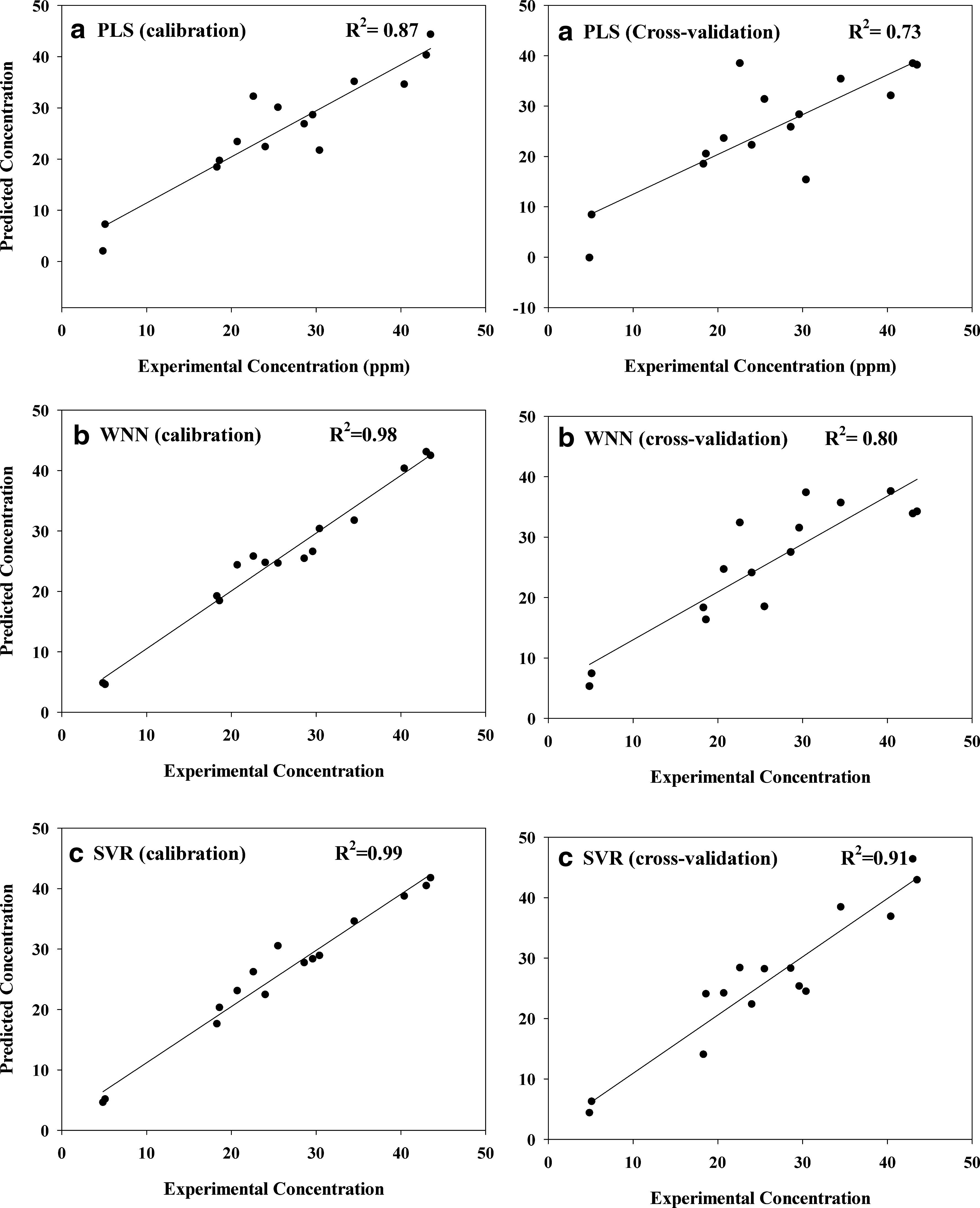
Figure 1a shows the relationship between experimental and PLS-predicted C_e for calibration and cross-validation modes. The plots with high values of R² and the random distribution of the residuals suggest appropriateness of the model. Figure 2a shows the residuals plot for PLS model, which can be more informative regarding model fitting to a data set. Figure 2a shows a random pattern in distribution of the residuals and suggests that the PLS model fits all the data points appropriately well.

FIG. 1.

Experimental versus calculated values of nickel (Ni) concentration for calibration and cross-validation in (a) PLS, (b) WNN, and (c) SVR models. SVR, support vector regression.

FIG. 2.

Residual plots for (a) PLS, (b) WNN, and (c) SVR models.

The results of the predicted C_e using LOO are presented in Table 1. It can be seen that the predicted values are not in good agreement with the experimental ones.

In addition, the PLS model was run for the complete calibration data set using the five LVs. The model's performance criteria are summarized in Table 2. The five LVs yielded the RMSEC and RMSECV values of 5.45 and 6.78, respectively (Table 2) with an R² of 0.86 and q² of 0.73. According to Table 2, regression coefficients are quite low. In addition, there is too much difference between R² and q², which obviously indicates that the correlation is poor, the response seems to be nonlinear, and the PLS model is inapplicable to adsorption studies.

Table 2.

Statistical Parameters for the Developed Calibration, Cross-Validation, and Prediction Models

	Calibration		Cross-validation			Prediction
Model	RMSEC	R²	RMSECV	RMSECVi	q²	RMSEP
PLS	5.45	0.87	6.78	6.33	0.73	7.89
WNN	2.58	0.98	5.18	5.05	0.80	6.29
SVR	2.50	0.99	3.64	3.52	0.91	4.52

RMSEC, root mean squared error of calibration; RMSECV, root mean squared error of cross-validation; RMSECVi; RMSEP, root mean squared error of prediction.

The calibrated model was applied to the test data set for prediction of C_e of Ni. The root mean squared error of prediction (RMSEP) is shown in Table 2. The PLS model yielded an RMSEP value of 7.89.

WNN model

The experimental values of C_e of Ni were plotted against the predicted ones by the WNN model (Fig. 1b). The R² of calibration was 0.98, and the q² of cross-validation was 0.80.

Figure 2b shows the residual plot, which reveals the appropriateness of WNN model in comparison with the PLS model. The values of RMSEC, RMSECV, and RMSECVi for the constructed model are shown in Table 2. According to Table 2, these three values are comparable, which means that the model is appropriate. It can be seen that according to all criteria, the WNN model is better than the PLS model.

In the next step, the constructed model was used to predict the C_e of Ni. The predicted values and the absolute errors are shown in Table 1. According to this table, there is a good agreement between experimental concentrations and the predicted ones using the WNN model. The RMSEP of this model was 6.29, which is lower than the PLS model (Table 2). This means that the correlation between parameters and C_e of Ni is not linear, and there is some nonlinearity in the system which may be modeled better with a nonlinear function.

Figure 3 shows the plot for different combinations of momentum and learning rate. It can be seen that the RMSE has its minimum value for all the tested combinations when the number of neurons in the hidden layer was eight.

FIG. 3.

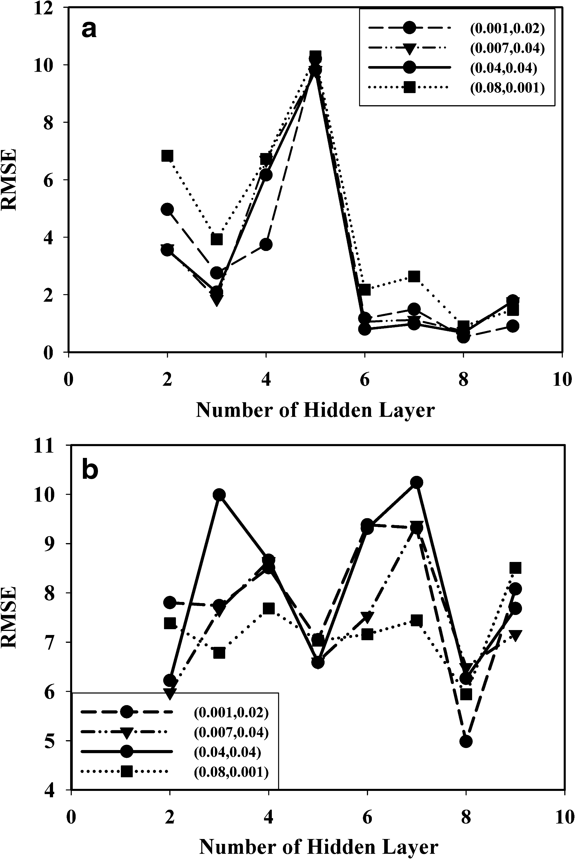
RMSE versus number of hidden layers for (a) calibration and (b) cross-validation in WNN model using different combinations of momentum values and learning rates.

The RMSE against different numerical values of momentum and learning rate are plotted in Fig. 4. According to this figure, some large values of RMSEC and RMSECV prevent distinguishing the best point graphically. However, according to the values of errors, the optimized values of momentum and learning rate were 0.0055 and 0.078, respectively.

FIG. 4.

Plots of: (a) momentum versus the index number, (b) learning rate versus the index number, (c) RMSE of calibration versus the index number, and (d) RMSE of cross-validation versus the index number.

In the next step, the number of iterations should be optimized for constructing the model. Figure 5 shows the RMSEC and RMSECV in different iterations. This figure shows that the RMSE decreases for the calibration set when the number of iterations increases from 100 to 15,000. However, the RMSE increases for cross-validation when the number of iterations increases from 2,000. Therefore, the optimum number of iterations is selected as 2,000 to prevent over-fitting of the model.

FIG. 5.

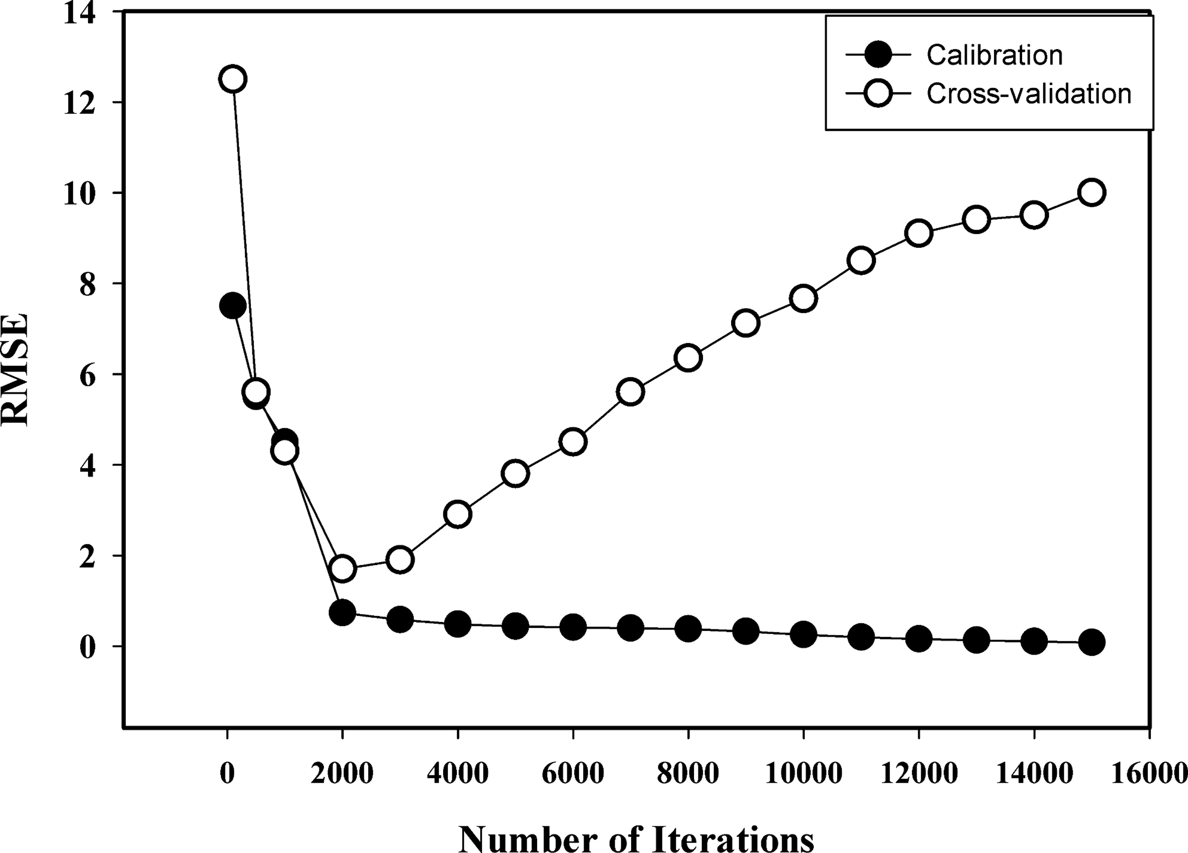
Variation of RMSE versus number of iterations for calibration and cross-validation in the WNN model.

SVR model

The predicted C_e of Ni against the experimental ones for calibration and cross-validation modes of the SVR model are plotted in Fig. 1c. In addition, the main statistical parameters of the LS-SVR model are listed in Table 2. According to this table, the values of RMSEC, RMSECV, and RMSECVi are comparable. These results suggest that both interpolations and extrapolations of C_e values by the SVR model are reasonably adequate. The high calculated q² of 0.91, and the low value of RMSECV of 3.64, as compared with the RMSEC of 2.5, suggests a good internal consistency as well as the predictive ability of the SVR model. The C_e of Ni predicted by LOO cross-validation are listed in Table 1. As can be seen, the predicted C_e are in good agreement with the experimental values. It is shown in Table 2 that RMSEP is 4.52 for the SVR model. The residual plot of SVR (Fig. 2c) shows a random pattern, which again confirms the suitability of the SVR model.

Figure 6 shows RMSEC and RMSECV for different γ and σ² values. As shown, the optimized parameters are not the same for all the points in both calibration and cross-validation graphs. However, the optimized values should be selected based on the minimum values for both criteria. The level of errors for RMSEC (Fig. 6a) and RMSECV (Fig. 6b) tends to a minimum value as σ² and γ decrease toward 100, and, therefore, the optimized σ² and γ were selected as 100. The RMSEC and RMSECV were 2.75 and 3.74, respectively, for these selected hyperparameters.

FIG. 6.

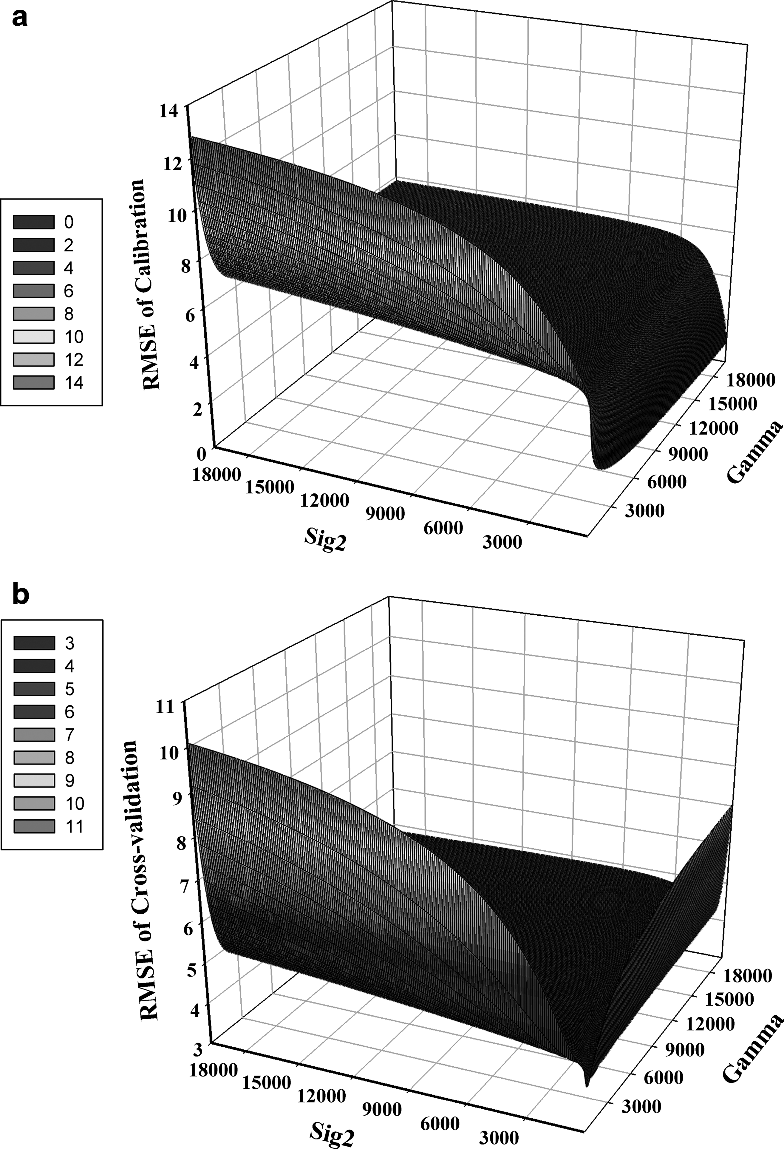
Tuning of γ and σ² for LS-SVR. (a) RMSE of calibration for different values of γ and σ², and (b) RMSE of cross-validation for different values of γ and σ².

In the next step, the parameters were optimized using the grid search method. This method gave the optimized values of 73.47 and 48.72, respectively, for γ and σ². The corresponding RMSEC and RMSECV to these values of hyperparameters were 2.50 and 3.64. The results are comparable for the proposed method and grid search, but the grid search has slightly better results. Additionally, it can be concluded that the grid search is a fast and effective method to optimize the hyperparameters in SVR modeling.

Comparison of the models

According to Tables 1 and 2, the SVR and WNN models have similar calibration statistics, but they differed in stability and prediction capability as measured by cross-validation using the external prediction set. The PLS model had weaker results in this respect as compared with the WNN and SVR models.

The cross-validation statistics of the SVR model were similar to those of calibration, which indicates the stability of this model. A weaker cross-validation performance was observed for the WNN model. The results of external predictions also support the fact that the SVR represented better prediction results than the WNN, whereas the WNN produced better results than the PLS.

According to the explanations just mentioned, it can be concluded that the performance of nonlinear calibration methods (SVR and WNN) in the prediction of adsorption of Ni to sunflower stalks is superior to the linear method (PLS model), whereas among the two nonlinear regression methods, the SVR represented slightly better prediction results.

Effect of the variables

In order to investigate the effect of variables (i.e., pH, contact time, dose of the adsorbent, and C_i of Ni), the SVM and WNN models were used. The models were constructed using all four variables, and then, the effect of each variable was evaluated by omitting it from the model. The RMSECV was calculated for the constructed models.

Figure 7 shows the results of this process. It can be seen that for both SVR and WNN models, the maximum increment of RMSECV was due to C_i, followed by pH, contact time, and dose of the adsorbent. This result has been previously proved, because at a low concentration, the ratio of available surface to the adsorbate ion concentration is larger; so, the removal is higher. However, in case of higher concentrations, this ratio is low; hence, the percentage removal is also less, and, therefore, the removal of Ni is dependent on the C_i (Jain et al., 2009).

FIG. 7.

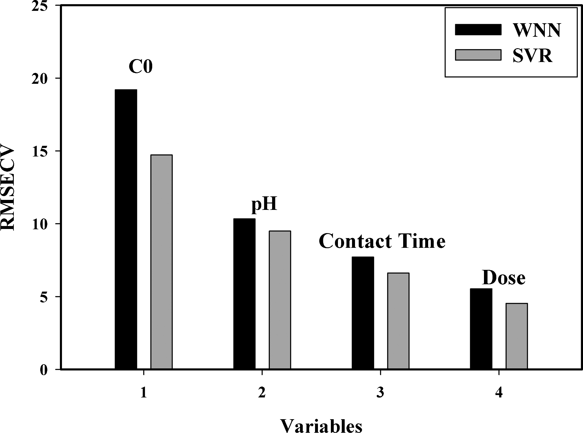
Histogram of RMSECV corresponding to omitting different variables from the WNN and SVM models.

The second effective parameter was the solution pH. pH is among the important parameters for adsorption process. Experimental results showed that the amount of Ni removal was relatively low at a pH less than 2.0. This may be due to the fact that at a pH lower than 3.0, high concentrations of H⁺ ions compete with Ni for active sites, which results in the suppression of Ni adsorption on the surface of sunflower stalks. In addition, this batch experiment showed that adsorption of Ni ions decreased when the pH was higher than 7.0. This can be attributed to the fact that a high pH condition reduces the mobility of Ni due to the decrease in the exchangeable form, resulting in a decrease in the contact probability between adsorbent and adsorbate (Yetilmezsoy and Demirel, 2008).

The third effective factor is contact time. Basically, removal of the adsorbate is rapid, but it gradually decreases with time until it reaches equilibrium. The experimental data showed that a contact time of 60 min is generally sufficient to achieve equilibrium, and the adsorption does not change significantly thereafter. In most cases, equilibrium was almost attained in 10 or 20 min, depending on the values of operating variables. Therefore, contact time has relatively the same effect in the model.

The fourth variable (dose of adsorbent) is less effective in the Ni adsorption process, which means that probably 0.5 g of sunflower stalks is enough for effective adsorption in this range of Ni concentration in the aqueous solution. According to Fig. 7, both SVR and WNN models gave similar results in the adsorption of Ni using sunflower stalks.

Conclusions

In this study, on the basis of batch adsorption experiments performed with four different process variables (pH, C_i of adsorbate, contact time, and dose of adsorbent), an important objective was to obtain a model that could make reliable prediction of C_e of Ni in wastewater using the sunflower stalks. The linear and nonlinear models included PLS, WNN, and SVR. These models were validated using the LOO cross-validation method. Performance of the selected models was evaluated using criteria such as RMSEC, RMSECV, R² for calibration, R² for cross-validation, and RMSE of prediction. All the three models predicted C_e of Ni satisfactorily. However, the performance of SVR and WNN nonlinear models was relatively better than that of the PLS model. The SVR model can be used as a powerful tool for modeling Ni removal using sunflower stalks. It was observed that there was an acceptable agreement between the SVR model results and experimental data.

Footnotes

Author Disclosure Statement

No competing financial interests exist.

References

Amarasinghe

B.M.W.P.K.

, Williams

R.A.

2007. Tea waste as a low cost adsorbent for the removal of Cu and Pb from wastewater. Chem. Eng. J., 132:299.

Basci

, Kocadagistan

2004. Biosorption of copper(II) from aqueous solutions by wheat shell. Desalination, 164:135.

Bhatnagar

, Sillanpaa

2010. Utilization of agro-industrial and municipal waste materials as potential adsorbents for water treatment—A review. Chem. Eng. J., 157:277.

Bhattacharya

A.K.

, Mandal

S.N.

, Das

S.K.

2006. Adsorption of Zn(II) from aqueous solution by using different adsorbents. Chem. Eng. J., 123:43.

Benaissa

, Elouchdi

M.A.

2007. Removal of copper ions from aqueous solutions by dried sunflower leaves. Chem. Eng. Proc., 46:614.

Chen

H.F.

2008. Computational study of histamine H3-receptor antagonist with support vector machines and three dimension quantitative structure activity relationship methods. Anal. Chim. Acta, 624:2039.

Duan

, Keerthi

S.S.

, Poo

A.N.

2003. Evaluation of simple performance measures for tuning SVM hyperparameters. Neurocomputing, 51:41.

Esteki

, Hemmateenejad

, Khayamian

, Mohajeri

2007. Multi-way analysis of quantum topological molecular similarity descriptors for modeling acidity constant of some phenolic compounds. Chem. Biol. Drug Design, 70:413.

Esteki

, Rezayat

, Ghaziaskar

H.S.

, Khayamian

2010. Application of QSPR for prediction of percent conversion of esterification reactions in supercritical carbon dioxide using least squares support vector regression. J. Supercrit. Fluids, 54:222.

10.

García-Reiriz

, Damiani

P.C.

, Culzoni

M.J.

, Goicoechea

H.C.

, Olivieri

A.C.

2008. A versatile strategy for achieving the second-order advantage when applying different artificial neural networks to non-linear second-order data: unfolded principal component analysis/residual bilinearization. Chemo. Intell. Lab. Sys., 92:61.

11.

Geladi

, Kowalski

B.R.

1986. Partial least squares (PLS) regression: A tutorial. Anal. Chim. Acta, 185:1.

12.

Hansen

H.K.

, Arancibia

, Gutierrez

2010. Adsorption of copper onto agriculture waste materials. J. Hazard. Mater., 180:442.

13.

Jain

, Garg

V.K.

, Kadirvelu

2009. Chromium(VI) removal from aqueous system using Heliantus annuus (sunflower) stem waste. J. Hazard. Mater., 162:365.

14.

Kang

Y.W.

, Li

, Cao

G.Y.

, Tu

H.Y.

, Li

, Yang

2008. Dynamic temperature modeling of a SOFC using least squares support vector machines. J. Power Sources, 179:683.

15.

Khambhaty

, Mody

, Basha

, Jha

2009. Biosorption of inorganic mercury onto dead biomass of marine Aspergillus niger: Kinetic, equilibrium, and thermodynamic studies. Environ. Eng. Sci., 26:531.

16.

Khayamian

, Esteki

2004. Prediction of solubility for polycyclic aromatic hydrocarbons in supercritical carbon dioxide using wavelet neural networks in quantitative structure property relationship. J. Supercrit. Fluids, 32:73.

17.

Liu

, He

, Wang

2008a. Comparison of calibrations for the determination of soluble solids content and pH of rice vinegars using visible and short-wave near infrared spectroscopy. Anal. Chim. Acta, 610:196.

18.

Liu

, He

, Wang

2008b. Determination of effective wavelengths for discrimination of fruit vinegars using near infrared spectroscopy and multivariate analysis. Anal. Chim. Acta, 615:10.

19.

Pan

, Jiang

, Wang

, Cao

2008. Advantages of support vector machine in QSPR studies for predicting auto-ignition temperatures of organic compounds. Chemo. Intell. Lab. Sys., 92:169.

20.

Park

, Yun

Y.S.

, Jo

J.H.

, Park

J.M.

2006. Biosorption process for treatment of electroplating wastewater containing Cr(VI): Laboratory-scale feasibility test. Ind. Eng. Chem. Res., 45:5059.

21.

Prakash

, Manikandan

S.A.

, Govindarajan

, Vijayagopal

2008. Prediction of biosorption efficiency for the removal of copper(II) using artificial neural networks. J. Hazard. Mater., 152:1268.

22.

Quinones-Torrelo

, Sagrado

, Villanueva-Camanas

R.M.

, Medina-Hernandez

M.J.

1999. Development of predictive retention-activity relationship models of tricyclic antidepressants by micellar liquid chromatography. J. Med. Chem., 42:3154.

23.

Romera

, Gonzalez

, Ballester

, Bllazquez

M.L.

, Munoz

J.A.

2008. Biosorption of Cd, Ni and Zn with mixtures of different types of algae. Environ. Eng. Sci., 25:999.

24.

Sahinkaya

2009. Biotreatment of zinc-containing wastewater in a sulfidogenic CSTR: Performance and artificial neural network (ANN) modelling studies. J. Hazard. Mater., 164:105.

25.

Smola

A.J.

, Scholkopf

1998. A Tutorial on Support Vector Regression. London: NeuroCOLT Technical Report NC-TR-98-030, University of London.

26.

Sun

, Shi

1998. Sunflower stalks as adsorbents for the removal of metal ions from wastewater. Ind. Eng. Chem. Res., 37:1324.

27.

Suykens

J.A.K.

, Van Gestel

, De Brabanter

, De Moor

, Vandewalle

2002. Least Squares Support Vector Machines. Singapore: World Scientific.

28.

Vapnik

1998. Statistical Learning Theory. New York: Wiley.

29.

Yetilmezsoy

, Demirel

2008. Artificial neural network (ANN) approach for modeling of Pb(II) adsorption from aqueous solution by Antep pistachio (Pistacia Vera L.) shells. J. Hazard. Mater., 153:1288.

30.

Zhang

, Banks

2006. A comparison of the properties of polyurethane immobilized Sphagnum moss, seaweed, sunflower waste and maize for the biosorption of Cu, Pb, Zn and Ni in continuous flow packed columns. Water Res., 40:788.

31.

Zhang

, Qi

, Zhang

, Liu

, Hu

, Xue

, Fan

2001. Prediction of programmed-temperature retention values of naphthas by wavelet neural network. Comput. Chem., 25:125.

32.

Zhong

, Zhang

, Gao

, Zheng

, Li

, Chen

2001. The discrete wavelet neural network and its application in oscillographic chronopotentiometric determination. Chemo. Intell. Lab. Syst., 59:67.