New Nonisothermal Arrhenius Temperature Integral Approximate Formula

Abstract

A new formula for approximating the Arrhenius temperature integral for nonisothermal analysis has been developed, using the Solver algorithm. The new formula takes the form p(u)=(e^−u/u²)×[(1−2/u)/(1−λ/u²)], where λ=0.33 ln(u)+4.48. Applicability of the formula has been proven by conducting thermogravimetric analysis experiments on polypropylene material. When simulated thermogravimetric analysis curves derived from the proposed approximation were compared with curves obtained from other published approximate formulae, the new approximation fit the experimental data very well. Numerical analysis was used to test accuracy of the proposed formula, and its deviation from the numerical value was compared with those of other published approximation formulae. Results show that the new formula is a suitable solution for the evaluation of kinetic parameters for nonisothermal kinetic analysis, for example, pyrolysis of polymeric wastes and biomass fuel or to produce biomass fuel. Its use will result in significant improvement in plastic resource recycling and could also be helpful in biomass energy production.

Introduction

Kujirai and Akahira (1925) were the first to publish a thermogravimetric analysis (TGA) of six fibrous insulating materials. Since then, TGA has been used extensively for studying the kinetics of solid state decomposition, for example, biomass pyrolysis (Van de Velden et al., 2008, 2010), polymeric waste (Brems et al., 2011a, 2011b), pollution (Rodríguez-Barroso, 2009), and fuel (Butterman and Castaldi, 2009, 2010). TGA kinetic analysis is usually based on the analysis of the conversion curves obtained from TGA. The rate of conversion obtained from conversion curve can be expressed as \documentclass{aastex}\usepackage{amsbsy}\usepackage{amsfonts}\usepackage{amssymb}\usepackage{bm}\usepackage{mathrsfs}\usepackage{pifont}\usepackage{stmaryrd}\usepackage{textcomp}\usepackage{portland, xspace}\usepackage{amsmath, amsxtra}\pagestyle{empty}\DeclareMathSizes{10}{9}{7}{6}\begin{document} \begin{align*} \frac { d \alpha } { { \rm d } t } = A \exp \left( \frac { - E } { RT } \right) \cdot f ( \alpha ) \tag { 1 } \end{align*} \end{document}

where t is time (sec); T, temperature (K); α, the conversion of reaction; f(α), the conversion function reflecting the mechanism of the process; A, the pre-exponential factor (K⁻¹); E, the activation energy (Kcal mol⁻¹); and R, the gas constant. For a nonisothermal and constant heating rate (β) condition, the following expression is obtained by integration and separation of variables of Equation (1), \documentclass{aastex}\usepackage{amsbsy}\usepackage{amsfonts}\usepackage{amssymb}\usepackage{bm}\usepackage{mathrsfs}\usepackage{pifont}\usepackage{stmaryrd}\usepackage{textcomp}\usepackage{portland, xspace}\usepackage{amsmath, amsxtra}\pagestyle{empty}\DeclareMathSizes{10}{9}{7}{6}\begin{document} \begin{align*}g ( \alpha ) = \int \limits_0^ { \partial } \frac { {\rm d} \alpha } { f ( \alpha ) } = \frac { A } { \beta } \int \limits_0^T \exp \left( \frac { - E } { RT } \right) { \rm d } T = \frac { AE } { \beta { R } } { p } ( u ) \tag { 2 } \end{align*} \end{document}

where u= E/RT, and p(u) is the Arrhenius temperature integral. As the Arrhenius temperature integral has no exact analytical solution, extensive efforts have been devoted to obtaining its approximation. Flynn (1997) published an excellent article introducing different types of Arrhenius temperature integral approximation formulae and pointing out that there are many articles available of varying complexity and accuracy. Heal (1999) suggested a way to evaluate Arrhenius temperature integral approximation formulae and noted that many approximate solutions are gross or inaccurate.

We proposes a new Arrhenius temperature integral formula that is simple, accurate, and can be used over a wide range of u values.

Theory and Calculation

The Arrhenius temperature integral, p(u), in Equation (2) can also be expressed as \documentclass{aastex}\usepackage{amsbsy}\usepackage{amsfonts}\usepackage{amssymb}\usepackage{bm}\usepackage{mathrsfs}\usepackage{pifont}\usepackage{stmaryrd}\usepackage{textcomp}\usepackage{portland, xspace}\usepackage{amsmath, amsxtra}\pagestyle{empty}\DeclareMathSizes{10}{9}{7}{6}\begin{document} \begin{align*} & p(u) = \int \limits_ { \infty } ^u - \frac { e^ { - u } } { u^2 } { \rm d } u \tag { 3 } \\& = \frac { e^ { - u } } { u^2 } \bigg |_ { \infty } ^u - \int \limits_ { \infty } ^u \frac { - 2e^ { - u } } { u^3 } { \rm d } u = \frac { e^ { - u } } { u^2 } - \int \limits_ { \infty } ^u \frac { - 2e^ { - u } } { u^3 } { \rm d } u \tag { 4 } \\& = \frac { e^ { - u } } { u^2 } - \int \limits_ { \infty } ^u 2u^ { - 3 } { \rm d } e^ { - u } = \frac { e^ { - u } } { u^2 } - 2 \frac { e^ { - u } } { u^3 } + \int \limits_ { \infty } ^u \frac { 6e^ { - u } } { u^4 } { \rm d } u \tag { 5 } \end{align*} \end{document}

The integral on the right-hand side of Equation (3) is an incomplete gamma function. It is not integrable and can only be approached numerically. Normally, the gamma function is solved either by the series solution (Rainville, 1960) or by numerical integration (Gyulai and Greenhow, 1974). However, neither solution provides a simple yet easily interpreted form for thermogravimetric analysis. The classic approximation of the Arrhenius temperature integral is the Coats and Redfern (1964) approximation, shown here as Equation (6). \documentclass{aastex}\usepackage{amsbsy}\usepackage{amsfonts}\usepackage{amssymb}\usepackage{bm}\usepackage{mathrsfs}\usepackage{pifont}\usepackage{stmaryrd}\usepackage{textcomp}\usepackage{portland, xspace}\usepackage{amsmath, amsxtra}\pagestyle{empty}\DeclareMathSizes{10}{9}{7}{6}\begin{document} \begin{align*} p (u) = \frac {e^{- u}} {u^2} \left(1 - \frac {2} {u} \right) \tag {6} \end{align*} \end{document}

Rearranging Equations (3) and (4), one obtains \documentclass{aastex}\usepackage{amsbsy}\usepackage{amsfonts}\usepackage{amssymb}\usepackage{bm}\usepackage{mathrsfs}\usepackage{pifont}\usepackage{stmaryrd}\usepackage{textcomp}\usepackage{portland, xspace}\usepackage{amsmath, amsxtra}\pagestyle{empty}\DeclareMathSizes{10}{9}{7}{6}\begin{document} \begin{align*} \int \limits_{\infty}^{- u} - \frac {e^{- u}} {u^2} \left(1 + \frac {2} {u} \right) du = \frac {e^{- u}} {u^2} \tag {7} \end{align*} \end{document}

Assuming the term (1+2/u) in Equation (7) is approximate to one and taking this term outside the integration part, Equation (7) can be rewritten as \documentclass{aastex}\usepackage{amsbsy}\usepackage{amsfonts}\usepackage{amssymb}\usepackage{bm}\usepackage{mathrsfs}\usepackage{pifont}\usepackage{stmaryrd}\usepackage{textcomp}\usepackage{portland, xspace}\usepackage{amsmath, amsxtra}\pagestyle{empty}\DeclareMathSizes{10}{9}{7}{6}\begin{document} \begin{align*} p (u) = \frac {e^{- u}} {u^2} \frac {1} {\left(1 + \displaystyle \frac {2} {u} \right)} = \frac {e^{- u}} {u^2} \frac {1 - \displaystyle \frac {2} {u}} {\left(1 - \displaystyle \frac {4} {u^2} \right)} \tag {8} \end{align*} \end{document}

which is the approximation equation proposed by Gorbachev (1977).

Using the same mathematic transformation, Li's approximation formula (Li, 1985) can be obtained by rearranging Equations (3) and (5) \documentclass{aastex}\usepackage{amsbsy}\usepackage{amsfonts}\usepackage{amssymb}\usepackage{bm}\usepackage{mathrsfs}\usepackage{pifont}\usepackage{stmaryrd}\usepackage{textcomp}\usepackage{portland, xspace}\usepackage{amsmath, amsxtra}\pagestyle{empty}\DeclareMathSizes{10}{9}{7}{6}\begin{document} \begin{align*} p (u) = \frac {e^{- u}} {u^2} \frac {1 - \displaystyle \frac {2} {u}} {\left(1 - \displaystyle \frac {6} {u^2} \right)} \tag {9} \end{align*} \end{document}

After comparing the Gorbachev and Li formulae, Agrawal (1987) replaced the coefficient of the term 1/u² in the denominator and developed his own approximation formula: \documentclass{aastex}\usepackage{amsbsy}\usepackage{amsfonts}\usepackage{amssymb}\usepackage{bm}\usepackage{mathrsfs}\usepackage{pifont}\usepackage{stmaryrd}\usepackage{textcomp}\usepackage{portland, xspace}\usepackage{amsmath, amsxtra}\pagestyle{empty}\DeclareMathSizes{10}{9}{7}{6}\begin{document} \begin{align*} p (u) = \frac {e^{- u}} {u^2} \frac {1 - \displaystyle \frac {2} {u}} {\left(1 - \displaystyle \frac {5} {u^2} \right)} \tag {10} \end{align*} \end{document}

Eight years later, Quanyin and Su (1995) found that the only difference between Equations (7 )–(10) was the coefficient of the term 1/u² in the denominator. As shown in Equations (11) and (12), they proposed two formulae using new coefficients: \documentclass{aastex}\usepackage{amsbsy}\usepackage{amsfonts}\usepackage{amssymb}\usepackage{bm}\usepackage{mathrsfs}\usepackage{pifont}\usepackage{stmaryrd}\usepackage{textcomp}\usepackage{portland, xspace}\usepackage{amsmath, amsxtra}\pagestyle{empty}\DeclareMathSizes{10}{9}{7}{6}\begin{document} \begin{align*} p (u) &= \frac {e^{- u}} {u^2} \frac {1 - \displaystyle \frac {2} {u}} {\left(1 - \displaystyle \frac {5.2} {u^2} \right)} &(11) \\ p (u) &= \frac {e^{- u}} {u^2} \frac {1 - \displaystyle \frac {2} {u}} {\left(1 - \displaystyle \frac {4.6} {u^2} \right)} &(12) \end{align*} \end{document}

From Equations (6 )–(12), we found that these equations have the form of a rational function which can be generalized as \documentclass{aastex}\usepackage{amsbsy}\usepackage{amsfonts}\usepackage{amssymb}\usepackage{bm}\usepackage{mathrsfs}\usepackage{pifont}\usepackage{stmaryrd}\usepackage{textcomp}\usepackage{portland, xspace}\usepackage{amsmath, amsxtra}\pagestyle{empty}\DeclareMathSizes{10}{9}{7}{6}\begin{document} \begin{align*} p_{cal} (u) = \frac {e^{- u}} {u^2} \frac {1 - \displaystyle \frac {2} {u}} {\left(1 - \displaystyle \frac {\lambda} {u^2} \right)} \tag {13} \end{align*} \end{document}

where λ, a parameter, replaces the coefficient of the term 1/u² in the denominator. Values of λ range from 0 (Coats and Redfern, 1964) to 6 (Li, 1985), and the value u varies with different λ values (Fig. 1). This raises one interesting question: Should λ remain a constant or can it be a variable based on u?

FIG. 1.

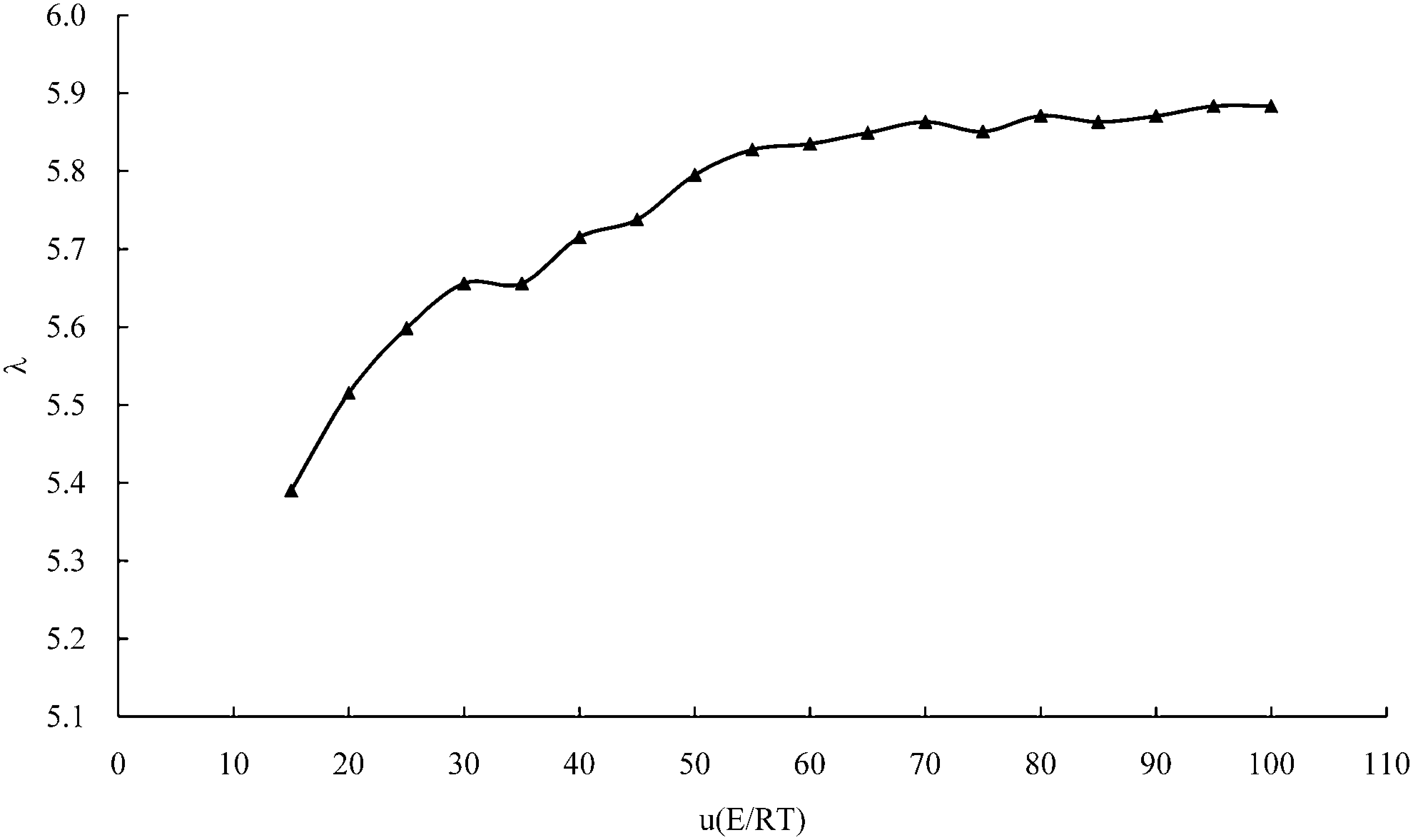
Relationship between u and λ.

In order to solve for λ, we utilized an algorithm called Solver. The Solver code, which is a product of Frontline System, Inc., is now a part of Microsoft Excel software (Billo, 2007). The value of λ for each u was determined by using Solver to find the best fit of the approximated temperature integral p(u) [Eq. (13)] to the numerical one. The numerical p(u) at each u was calculated with Mathematica software (Stephen, 2003). Table 1 shows the results of λ, u, ln(u) and numerical values of p(u) at different values of u. A close examination of the relationship between λ and u reveals an almost linear relationship between λ and ln(u) that can be illustrated by plotting λ against ln(u), as shown in Fig. 2. Through linear regression, we determined the y axis intercept, slope, and regression coefficient of the approximately straight line in Fig. 2 are 4.48, 0.33, and 0.98, respectively. Thus, λ can be represented as \documentclass{aastex}\usepackage{amsbsy}\usepackage{amsfonts}\usepackage{amssymb}\usepackage{bm}\usepackage{mathrsfs}\usepackage{pifont}\usepackage{stmaryrd}\usepackage{textcomp}\usepackage{portland, xspace}\usepackage{amsmath, amsxtra}\pagestyle{empty}\DeclareMathSizes{10}{9}{7}{6}\begin{document} \begin{align*} \lambda = 0.33 \ \ln (u) + 4.48 \tag{14} \end{align*} \end{document}

FIG. 2.

Plotting of λ vs. ln(u).

Table 1.

Results of λ, ln(u), and Numerical p (u) Values at Different Values of u

u	Numerical p(u)	λ	ln(u)
10	3.8302×10⁻⁷	5.1759	2.3026
15	1.2072×10⁻⁹	5.3902	2.7081
20	4.7024×10⁻¹²	5.5154	2.9957
25	2.0628×10⁻¹⁴	5.5983	3.2189
30	9.7656×10⁻¹⁷	5.6558	3.4012
35	4.8756×10⁻¹⁹	5.6558	3.5553
40	2.5315×10⁻²¹	5.7151	3.6889
45	1.3546×10⁻²³	5.7377	3.8067
50	7.4236×10⁻²⁶	5.7951	3.9120
55	4.1479×10⁻²⁸	5.8274	4.0073
60	2.3551×10⁻³⁰	5.8349	4.0943
65	1.3554×10⁻³²	5.8490	4.1744
70	7.8908×10⁻³⁵	5.8632	4.2485

The new approximation of p(u) can now take the form \documentclass{aastex}\usepackage{amsbsy}\usepackage{amsfonts}\usepackage{amssymb}\usepackage{bm}\usepackage{mathrsfs}\usepackage{pifont}\usepackage{stmaryrd}\usepackage{textcomp}\usepackage{portland, xspace}\usepackage{amsmath, amsxtra}\pagestyle{empty}\DeclareMathSizes{10}{9}{7}{6}\begin{document} \begin{align*} p_{cal} (u) = \frac {e^{- u}} {u^2} \frac {1 - \displaystyle \frac {2} {u}} {\left(1 - \displaystyle \frac {0.33 \ln (u) + 4.48} {u^2} \right)} \tag {15} \end{align*} \end{document}

Experimental verification

To prove the applicability of the new approximation of p(u), a commercial grade polypropylene from Formosa Plastics Corporation was used in a TGA experiment. The melting point and density of the polypropylene are 150°C–176°C and 0.918 g/cm³, respectively. Experiments were carried out on a METTLER TGA/SDTA 851 instrument in a nitrogen atmosphere with a flow rate of 50 mL/min.

Results and Discussions

The TG and DTG curves of the polypropylene are shown in Fig. 3. From an examination of the curves in Fig. 3, the pyrolysis reaction can be assumed to be a single-step reaction whose reaction model f(α) can be determined by the master plot method (Gotor et al., 2000).

FIG. 3.

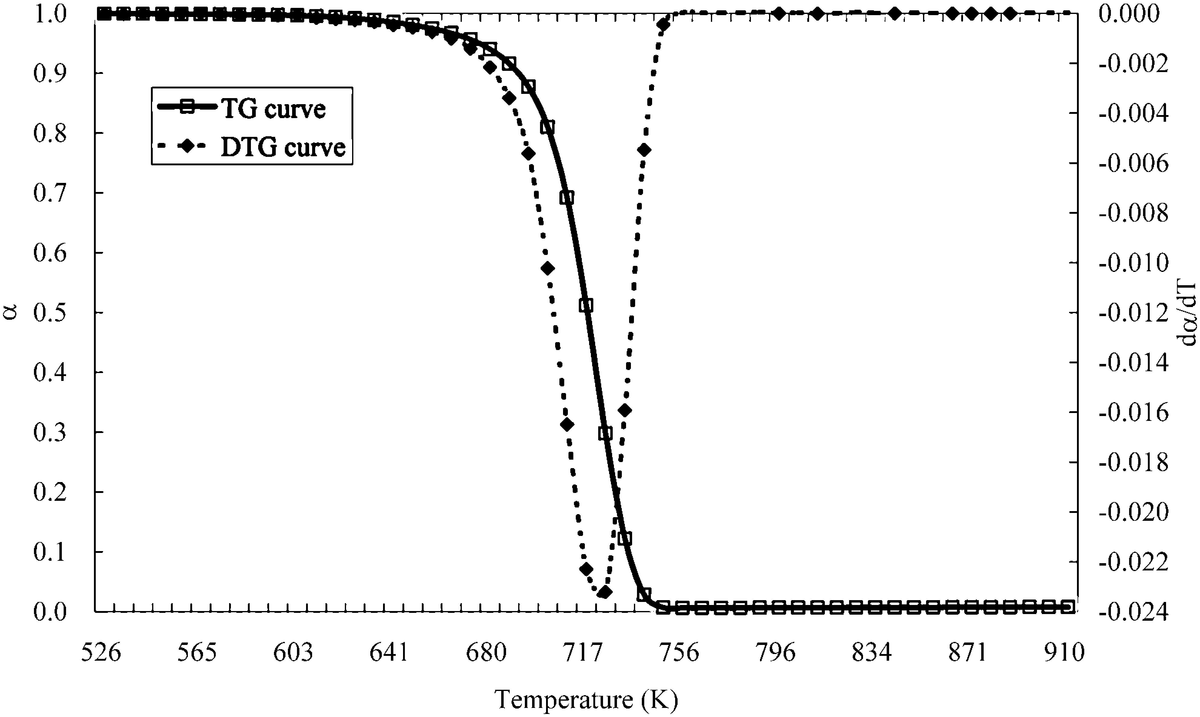
TG and DTG curves of polypropylene from TGA experiment.

For α=0.5, Equation (3) can be expressed as \documentclass{aastex}\usepackage{amsbsy}\usepackage{amsfonts}\usepackage{amssymb}\usepackage{bm}\usepackage{mathrsfs}\usepackage{pifont}\usepackage{stmaryrd}\usepackage{textcomp}\usepackage{portland, xspace}\usepackage{amsmath, amsxtra}\pagestyle{empty}\DeclareMathSizes{10}{9}{7}{6}\begin{document} \begin{align*}g ( 0.5 ) = \frac { { AE } } { \beta { R } } { p } ( u_ { 0.5 } ) \tag { 16 } \end{align*} \end{document}

where g(0.5) and p(u_0.5) are defined as the values of g(α) and p(u) at α=0.5, respectively.

By dividing Equation (2) by Equation (16), we obtain Equation (17): \documentclass{aastex}\usepackage{amsbsy}\usepackage{amsfonts}\usepackage{amssymb}\usepackage{bm}\usepackage{mathrsfs}\usepackage{pifont}\usepackage{stmaryrd}\usepackage{textcomp}\usepackage{portland, xspace}\usepackage{amsmath, amsxtra}\pagestyle{empty}\DeclareMathSizes{10}{9}{7}{6}\begin{document} \begin{align*} \frac {g (u)} {g (0.5)} = \frac {{p} (u)} {{p} (u_{0.5})} \tag {17} \end{align*} \end{document}

in which the value of p(u)/p(u_0.5) should be equal to the value of g(α)/g(0.5) if an appropriate kinetic model g(α) is chosen. To determine the appropriate kinetic model, two sets of plots need to be constructed. One is an experimental master plot that is defined by plotting p(u)/p(u_0.5) against α, and the other is a theoretical master plot that is defined by plotting g(α)/g(0.5) against α.

A set of theoretical master plots was constructed from different kinetic models, which are listed in Table 2. The experimental master plot was constructed from the new approximate p(u) function [Eq. (15)] with TGA experimental data and the activation energy, E, in u=E/RT, adopted from our previous work (Tai and Hsu, 2012). The same procedures were repeated for the other p(u) approximations (Coats-Redfern, Gorbachev, Li, Agrawal and Quanyin). The results are shown in Fig. 4. A comparison of the experimental master plots and the theoretical plots indicates that the most probably kinetic model for describing the nonisothermal solid decomposition of polypropylene is the Avrami-Erofeev model, g(α)=[−ln(1−α)]^1/m, because all experimental master plots in Figure 4 lie between the theoretical master plots A_1.5 and A₂. 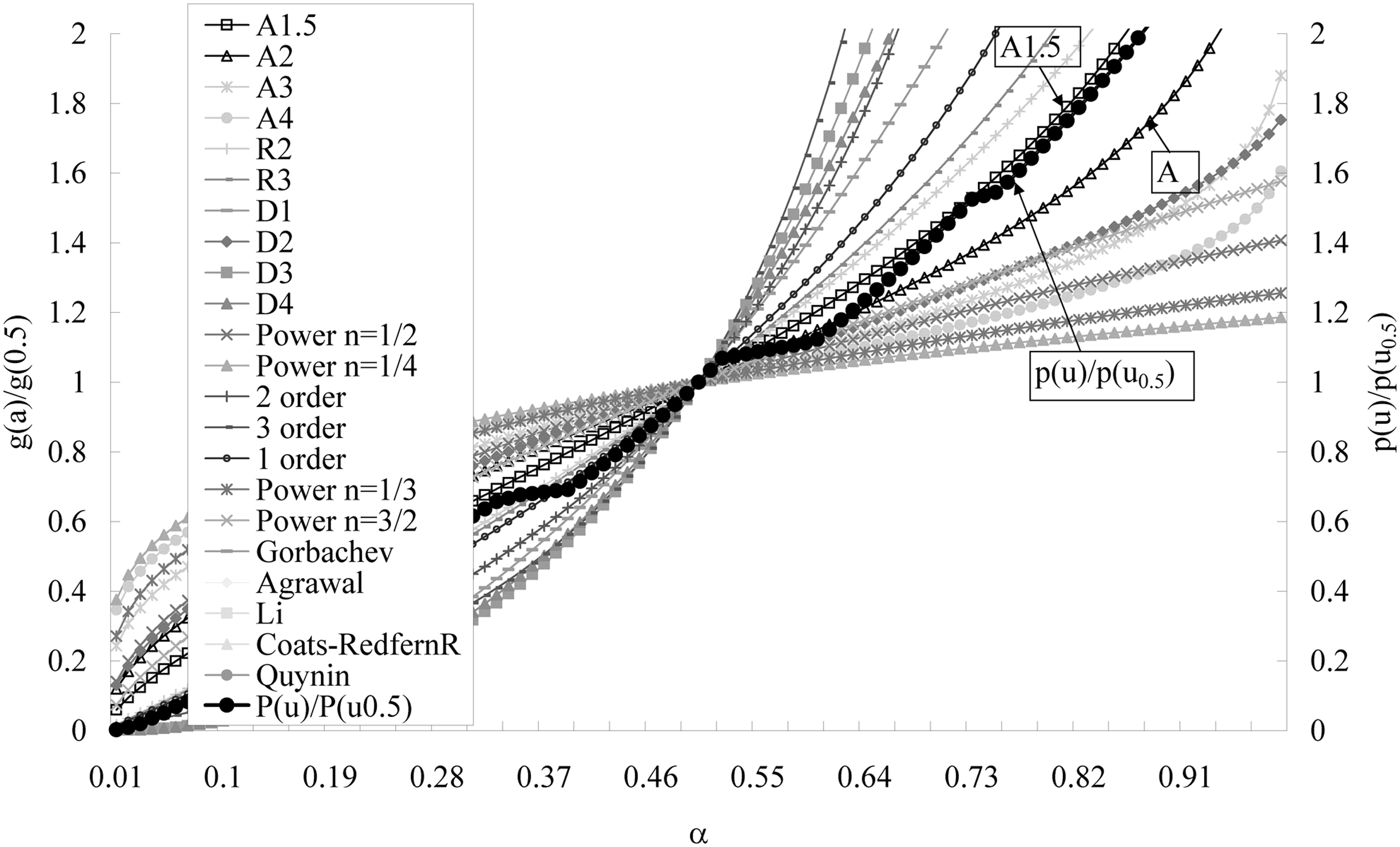By introducing g(α)=[−ln(1−α)]^1/m into Equation (2), the parameters of A and m can be determined, using the following equation: \documentclass{aastex}\usepackage{amsbsy}\usepackage{amsfonts}\usepackage{amssymb}\usepackage{bm}\usepackage{mathrsfs}\usepackage{pifont}\usepackage{stmaryrd}\usepackage{textcomp}\usepackage{portland, xspace}\usepackage{amsmath, amsxtra}\pagestyle{empty}\DeclareMathSizes{10}{9}{7}{6}\begin{document} \begin{align*} \ln \left[\frac {\beta R} {E} \right] - \ln [p (u)] = \ln A - \frac {1} {m} \cdot \ln [- \ln (1 - \alpha)] \tag {18} \end{align*} \end{document}

FIG. 4.

Comparison of experimental master plots and theoretical plots.

Table 2.

Expressions for f(α) and g(α) Functions for the Most Common Mechanism in Solid State Reactions

Mechanism	Symbol	g(α)	f(α)
Avrami-Erofeev	A_1.5	\documentclass{aastex}\usepackage{amsbsy}\usepackage{amsfonts}\usepackage{amssymb}\usepackage{bm}\usepackage{mathrsfs}\usepackage{pifont}\usepackage{stmaryrd}\usepackage{textcomp}\usepackage{portland, xspace}\usepackage{amsmath, amsxtra}\pagestyle{empty}\DeclareMathSizes{10}{9}{7}{6}\begin{document} $$[- \ln (1 - \alpha)]^\frac {2} {3}$$ \end{document}	\documentclass{aastex}\usepackage{amsbsy}\usepackage{amsfonts}\usepackage{amssymb}\usepackage{bm}\usepackage{mathrsfs}\usepackage{pifont}\usepackage{stmaryrd}\usepackage{textcomp}\usepackage{portland, xspace}\usepackage{amsmath, amsxtra}\pagestyle{empty}\DeclareMathSizes{10}{9}{7}{6}\begin{document} $$\displaystyle \frac {2} {3} (1 - \alpha) [- \ln (1 - \alpha)]^\frac {2} {3}$$ \end{document}
	A₂	\documentclass{aastex}\usepackage{amsbsy}\usepackage{amsfonts}\usepackage{amssymb}\usepackage{bm}\usepackage{mathrsfs}\usepackage{pifont}\usepackage{stmaryrd}\usepackage{textcomp}\usepackage{portland, xspace}\usepackage{amsmath, amsxtra}\pagestyle{empty}\DeclareMathSizes{10}{9}{7}{6}\begin{document} $$[- \ln (1 - \alpha)]^\frac {1} {2}$$ \end{document}	\documentclass{aastex}\usepackage{amsbsy}\usepackage{amsfonts}\usepackage{amssymb}\usepackage{bm}\usepackage{mathrsfs}\usepackage{pifont}\usepackage{stmaryrd}\usepackage{textcomp}\usepackage{portland, xspace}\usepackage{amsmath, amsxtra}\pagestyle{empty}\DeclareMathSizes{10}{9}{7}{6}\begin{document} $$2 (1 - \alpha) [- \ln (1 - \alpha)]^\frac {1} {2}$$ \end{document}
	A₃	\documentclass{aastex}\usepackage{amsbsy}\usepackage{amsfonts}\usepackage{amssymb}\usepackage{bm}\usepackage{mathrsfs}\usepackage{pifont}\usepackage{stmaryrd}\usepackage{textcomp}\usepackage{portland, xspace}\usepackage{amsmath, amsxtra}\pagestyle{empty}\DeclareMathSizes{10}{9}{7}{6}\begin{document} $$[- \ln (1 - \alpha)]^\frac {1} {3}$$ \end{document}	\documentclass{aastex}\usepackage{amsbsy}\usepackage{amsfonts}\usepackage{amssymb}\usepackage{bm}\usepackage{mathrsfs}\usepackage{pifont}\usepackage{stmaryrd}\usepackage{textcomp}\usepackage{portland, xspace}\usepackage{amsmath, amsxtra}\pagestyle{empty}\DeclareMathSizes{10}{9}{7}{6}\begin{document} $$3 (1 - \alpha) [- \ln (1 - \alpha)]^\frac {2} {3}$$ \end{document}
	A₄	\documentclass{aastex}\usepackage{amsbsy}\usepackage{amsfonts}\usepackage{amssymb}\usepackage{bm}\usepackage{mathrsfs}\usepackage{pifont}\usepackage{stmaryrd}\usepackage{textcomp}\usepackage{portland, xspace}\usepackage{amsmath, amsxtra}\pagestyle{empty}\DeclareMathSizes{10}{9}{7}{6}\begin{document} $$[- \ln (1 - \alpha)]^\frac {1} {4}$$ \end{document}	\documentclass{aastex}\usepackage{amsbsy}\usepackage{amsfonts}\usepackage{amssymb}\usepackage{bm}\usepackage{mathrsfs}\usepackage{pifont}\usepackage{stmaryrd}\usepackage{textcomp}\usepackage{portland, xspace}\usepackage{amsmath, amsxtra}\pagestyle{empty}\DeclareMathSizes{10}{9}{7}{6}\begin{document} $$4 (1 - \alpha) [- \ln (1 - \alpha)]^\frac {3} {4}$$ \end{document}
Phase boundary	R₂	\documentclass{aastex}\usepackage{amsbsy}\usepackage{amsfonts}\usepackage{amssymb}\usepackage{bm}\usepackage{mathrsfs}\usepackage{pifont}\usepackage{stmaryrd}\usepackage{textcomp}\usepackage{portland, xspace}\usepackage{amsmath, amsxtra}\pagestyle{empty}\DeclareMathSizes{10}{9}{7}{6}\begin{document} $$2 \left[1 - (1 - \alpha)^\frac {1} {2} \right]$$ \end{document}	\documentclass{aastex}\usepackage{amsbsy}\usepackage{amsfonts}\usepackage{amssymb}\usepackage{bm}\usepackage{mathrsfs}\usepackage{pifont}\usepackage{stmaryrd}\usepackage{textcomp}\usepackage{portland, xspace}\usepackage{amsmath, amsxtra}\pagestyle{empty}\DeclareMathSizes{10}{9}{7}{6}\begin{document} $$(1 - \alpha)^\frac {1} {2}$$ \end{document}
	R₃	\documentclass{aastex}\usepackage{amsbsy}\usepackage{amsfonts}\usepackage{amssymb}\usepackage{bm}\usepackage{mathrsfs}\usepackage{pifont}\usepackage{stmaryrd}\usepackage{textcomp}\usepackage{portland, xspace}\usepackage{amsmath, amsxtra}\pagestyle{empty}\DeclareMathSizes{10}{9}{7}{6}\begin{document} $$3 \left[1 - (1 - \alpha)^\frac {1} {3} \right]$$ \end{document}	\documentclass{aastex}\usepackage{amsbsy}\usepackage{amsfonts}\usepackage{amssymb}\usepackage{bm}\usepackage{mathrsfs}\usepackage{pifont}\usepackage{stmaryrd}\usepackage{textcomp}\usepackage{portland, xspace}\usepackage{amsmath, amsxtra}\pagestyle{empty}\DeclareMathSizes{10}{9}{7}{6}\begin{document} $$(1 - \alpha)^\frac {2} {3}$$ \end{document}
One-dimensional diffusion	D₁	\documentclass{aastex}\usepackage{amsbsy}\usepackage{amsfonts}\usepackage{amssymb}\usepackage{bm}\usepackage{mathrsfs}\usepackage{pifont}\usepackage{stmaryrd}\usepackage{textcomp}\usepackage{portland, xspace}\usepackage{amsmath, amsxtra}\pagestyle{empty}\DeclareMathSizes{10}{9}{7}{6}\begin{document} $$\displaystyle \frac {1} {2} \alpha^2$$ \end{document}	\documentclass{aastex}\usepackage{amsbsy}\usepackage{amsfonts}\usepackage{amssymb}\usepackage{bm}\usepackage{mathrsfs}\usepackage{pifont}\usepackage{stmaryrd}\usepackage{textcomp}\usepackage{portland, xspace}\usepackage{amsmath, amsxtra}\pagestyle{empty}\DeclareMathSizes{10}{9}{7}{6}\begin{document} $$\alpha^{- 1}$$ \end{document}
Two-dimensional diffusion	D₂	\documentclass{aastex}\usepackage{amsbsy}\usepackage{amsfonts}\usepackage{amssymb}\usepackage{bm}\usepackage{mathrsfs}\usepackage{pifont}\usepackage{stmaryrd}\usepackage{textcomp}\usepackage{portland, xspace}\usepackage{amsmath, amsxtra}\pagestyle{empty}\DeclareMathSizes{10}{9}{7}{6}\begin{document} $$\displaystyle \frac {1} {2} \left[1 - (1 - \alpha)^\frac {1} {2} \right]^\frac {1} {2}$$ \end{document}	\documentclass{aastex}\usepackage{amsbsy}\usepackage{amsfonts}\usepackage{amssymb}\usepackage{bm}\usepackage{mathrsfs}\usepackage{pifont}\usepackage{stmaryrd}\usepackage{textcomp}\usepackage{portland, xspace}\usepackage{amsmath, amsxtra}\pagestyle{empty}\DeclareMathSizes{10}{9}{7}{6}\begin{document} $$2 (1 - \alpha)^\frac {1} {2} \left[1 - (1 - \alpha)^\frac {1} {2} \right]^\frac {1} {2}$$ \end{document}
Three-dimensional diffusion	D₄	\documentclass{aastex}\usepackage{amsbsy}\usepackage{amsfonts}\usepackage{amssymb}\usepackage{bm}\usepackage{mathrsfs}\usepackage{pifont}\usepackage{stmaryrd}\usepackage{textcomp}\usepackage{portland, xspace}\usepackage{amsmath, amsxtra}\pagestyle{empty}\DeclareMathSizes{10}{9}{7}{6}\begin{document} $$1 - \displaystyle \frac {2} {3} \alpha - (1 - \alpha)^\frac {2} {3}$$ \end{document}	\documentclass{aastex}\usepackage{amsbsy}\usepackage{amsfonts}\usepackage{amssymb}\usepackage{bm}\usepackage{mathrsfs}\usepackage{pifont}\usepackage{stmaryrd}\usepackage{textcomp}\usepackage{portland, xspace}\usepackage{amsmath, amsxtra}\pagestyle{empty}\DeclareMathSizes{10}{9}{7}{6}\begin{document} $$\displaystyle \frac {2} {3} \left[(1 - \alpha)^\frac {- 1} {3} - 1 \right]^{- 1}$$ \end{document}
Jander diffusion	D₃	\documentclass{aastex}\usepackage{amsbsy}\usepackage{amsfonts}\usepackage{amssymb}\usepackage{bm}\usepackage{mathrsfs}\usepackage{pifont}\usepackage{stmaryrd}\usepackage{textcomp}\usepackage{portland, xspace}\usepackage{amsmath, amsxtra}\pagestyle{empty}\DeclareMathSizes{10}{9}{7}{6}\begin{document} $$\left[1 - (1 - \alpha)^\frac {1} {2} \right]^2$$ \end{document}	\documentclass{aastex}\usepackage{amsbsy}\usepackage{amsfonts}\usepackage{amssymb}\usepackage{bm}\usepackage{mathrsfs}\usepackage{pifont}\usepackage{stmaryrd}\usepackage{textcomp}\usepackage{portland, xspace}\usepackage{amsmath, amsxtra}\pagestyle{empty}\DeclareMathSizes{10}{9}{7}{6}\begin{document} $$\displaystyle \frac {2} {3} (1 - \alpha)^\frac {2} {3} \left[1 - (1 - \alpha)^\frac {1} {3} \right]^{- 1}$$ \end{document}
Power law	Power 1/2	\documentclass{aastex}\usepackage{amsbsy}\usepackage{amsfonts}\usepackage{amssymb}\usepackage{bm}\usepackage{mathrsfs}\usepackage{pifont}\usepackage{stmaryrd}\usepackage{textcomp}\usepackage{portland, xspace}\usepackage{amsmath, amsxtra}\pagestyle{empty}\DeclareMathSizes{10}{9}{7}{6}\begin{document} $$\alpha^\frac {1} {2}$$ \end{document}	\documentclass{aastex}\usepackage{amsbsy}\usepackage{amsfonts}\usepackage{amssymb}\usepackage{bm}\usepackage{mathrsfs}\usepackage{pifont}\usepackage{stmaryrd}\usepackage{textcomp}\usepackage{portland, xspace}\usepackage{amsmath, amsxtra}\pagestyle{empty}\DeclareMathSizes{10}{9}{7}{6}\begin{document} $$2 \alpha^\frac {1} {2}$$ \end{document}
	Power 1/3	\documentclass{aastex}\usepackage{amsbsy}\usepackage{amsfonts}\usepackage{amssymb}\usepackage{bm}\usepackage{mathrsfs}\usepackage{pifont}\usepackage{stmaryrd}\usepackage{textcomp}\usepackage{portland, xspace}\usepackage{amsmath, amsxtra}\pagestyle{empty}\DeclareMathSizes{10}{9}{7}{6}\begin{document} $$\alpha^\frac {1} {3}$$ \end{document}	\documentclass{aastex}\usepackage{amsbsy}\usepackage{amsfonts}\usepackage{amssymb}\usepackage{bm}\usepackage{mathrsfs}\usepackage{pifont}\usepackage{stmaryrd}\usepackage{textcomp}\usepackage{portland, xspace}\usepackage{amsmath, amsxtra}\pagestyle{empty}\DeclareMathSizes{10}{9}{7}{6}\begin{document} $$3 \alpha^\frac {1} {3}$$ \end{document}
	Power 1/4	\documentclass{aastex}\usepackage{amsbsy}\usepackage{amsfonts}\usepackage{amssymb}\usepackage{bm}\usepackage{mathrsfs}\usepackage{pifont}\usepackage{stmaryrd}\usepackage{textcomp}\usepackage{portland, xspace}\usepackage{amsmath, amsxtra}\pagestyle{empty}\DeclareMathSizes{10}{9}{7}{6}\begin{document} $$\alpha^\frac {1} {4}$$ \end{document}	\documentclass{aastex}\usepackage{amsbsy}\usepackage{amsfonts}\usepackage{amssymb}\usepackage{bm}\usepackage{mathrsfs}\usepackage{pifont}\usepackage{stmaryrd}\usepackage{textcomp}\usepackage{portland, xspace}\usepackage{amsmath, amsxtra}\pagestyle{empty}\DeclareMathSizes{10}{9}{7}{6}\begin{document} $$4 \alpha^\frac {1} {4}$$ \end{document}

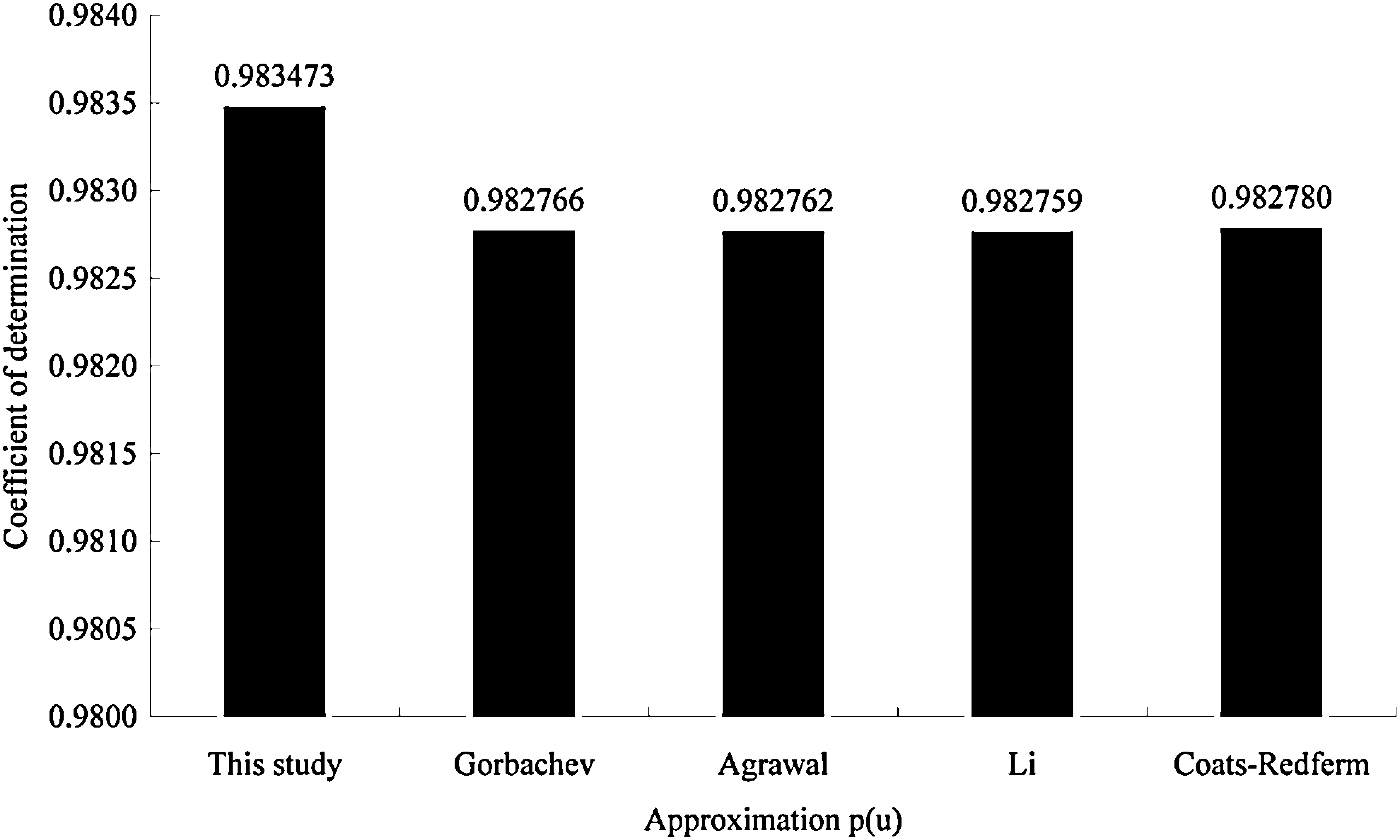
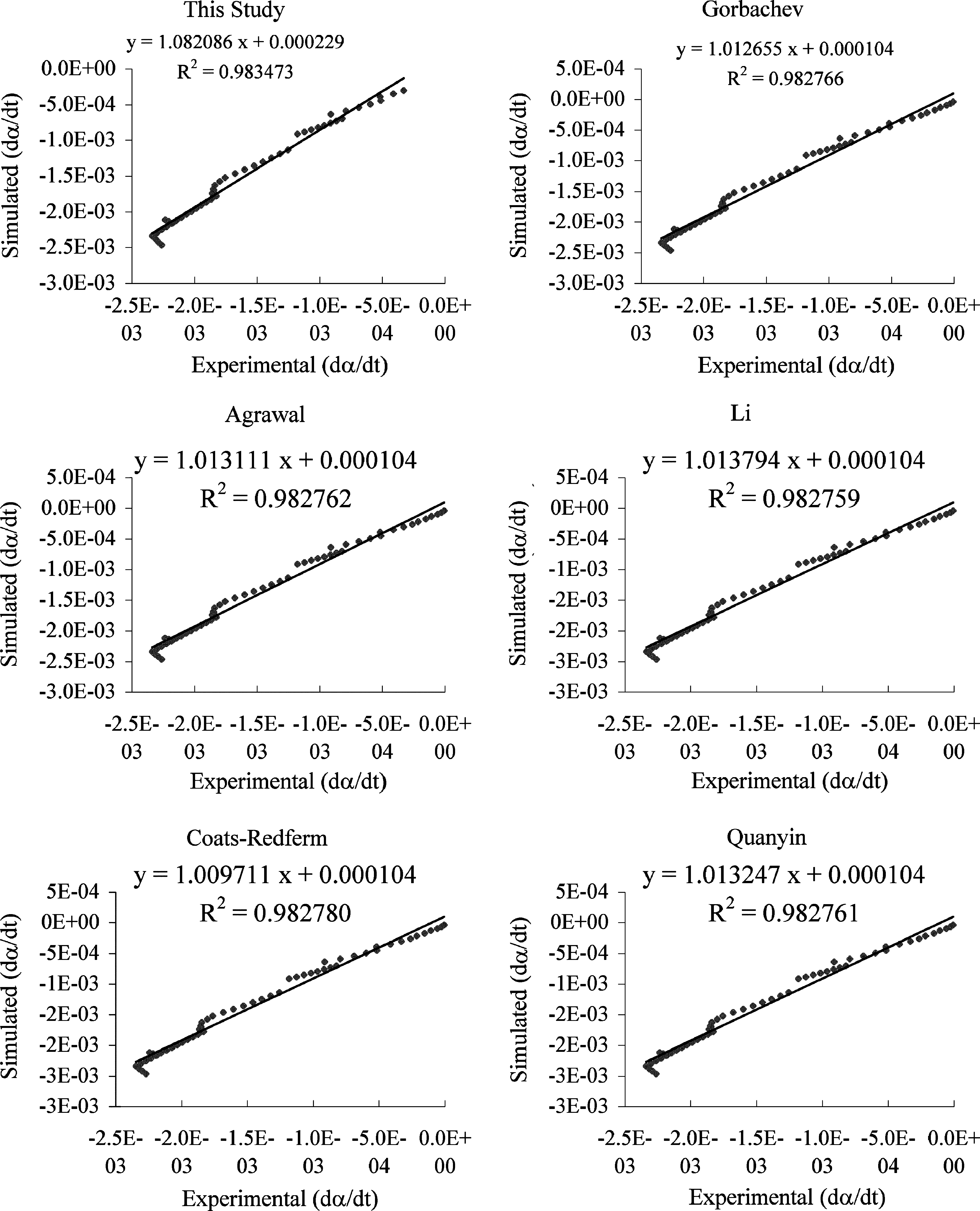
Figure 5 shows the plotting of ln(βR/E)−ln[p(u)] against ln[−ln(1−α)]. The pre-exponential factor A can be obtained from the intercept (ln A) on the y axis and the values of m can be obtained from the slopes (−1/m). The results of m and A are summarized in Table 3. The simulated DTG curves, which are shown in Fig. 6, were constructed by introducing parameters A and m into Equation (3). To examine the fitness of all simulated DTG data, the coefficient of determination, r², was calculated. Figure 7 shows the linearity between the experimental and simulated DTG data. The results of the coefficient of determination, r², shown in Fig. 8, indicate that the simulated values obtained from our approximation equation fit the experimental data as well as the values obtained from the other approximation equations.

FIG. 5.

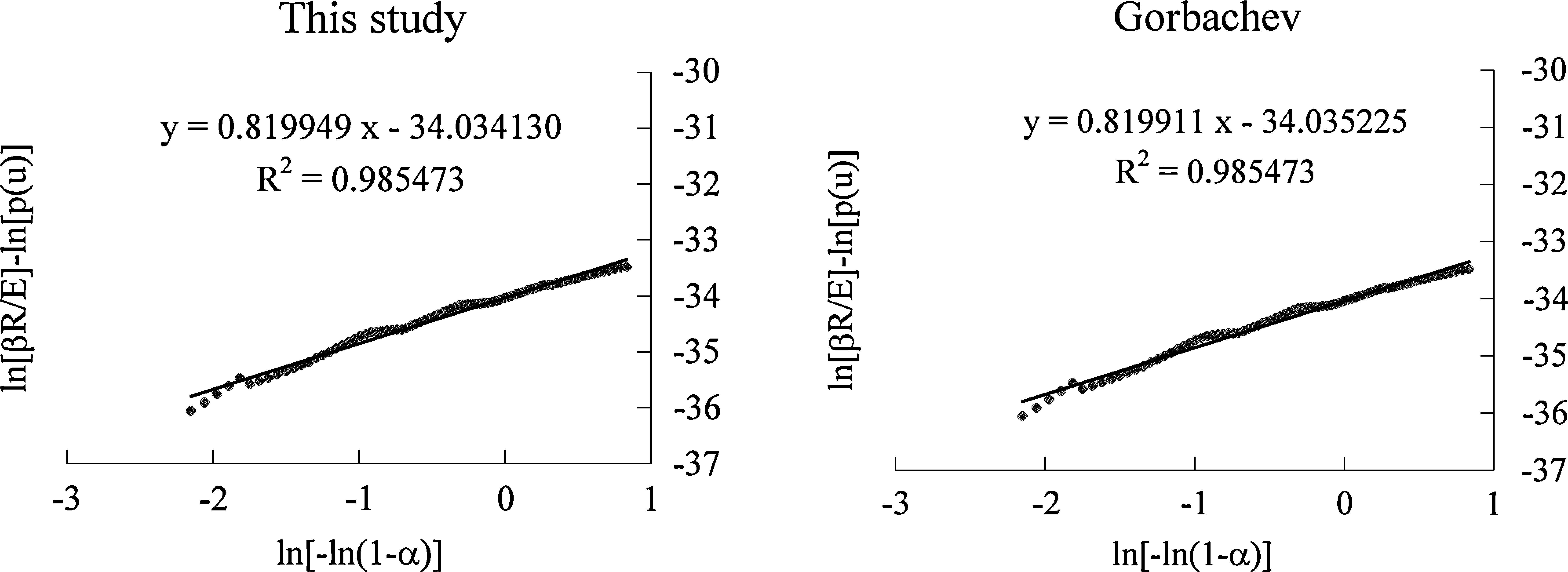
The plotting of ln(βR/E)−ln[p(u)] against ln[−ln(1−α)]. (continued)

FIG. 6.

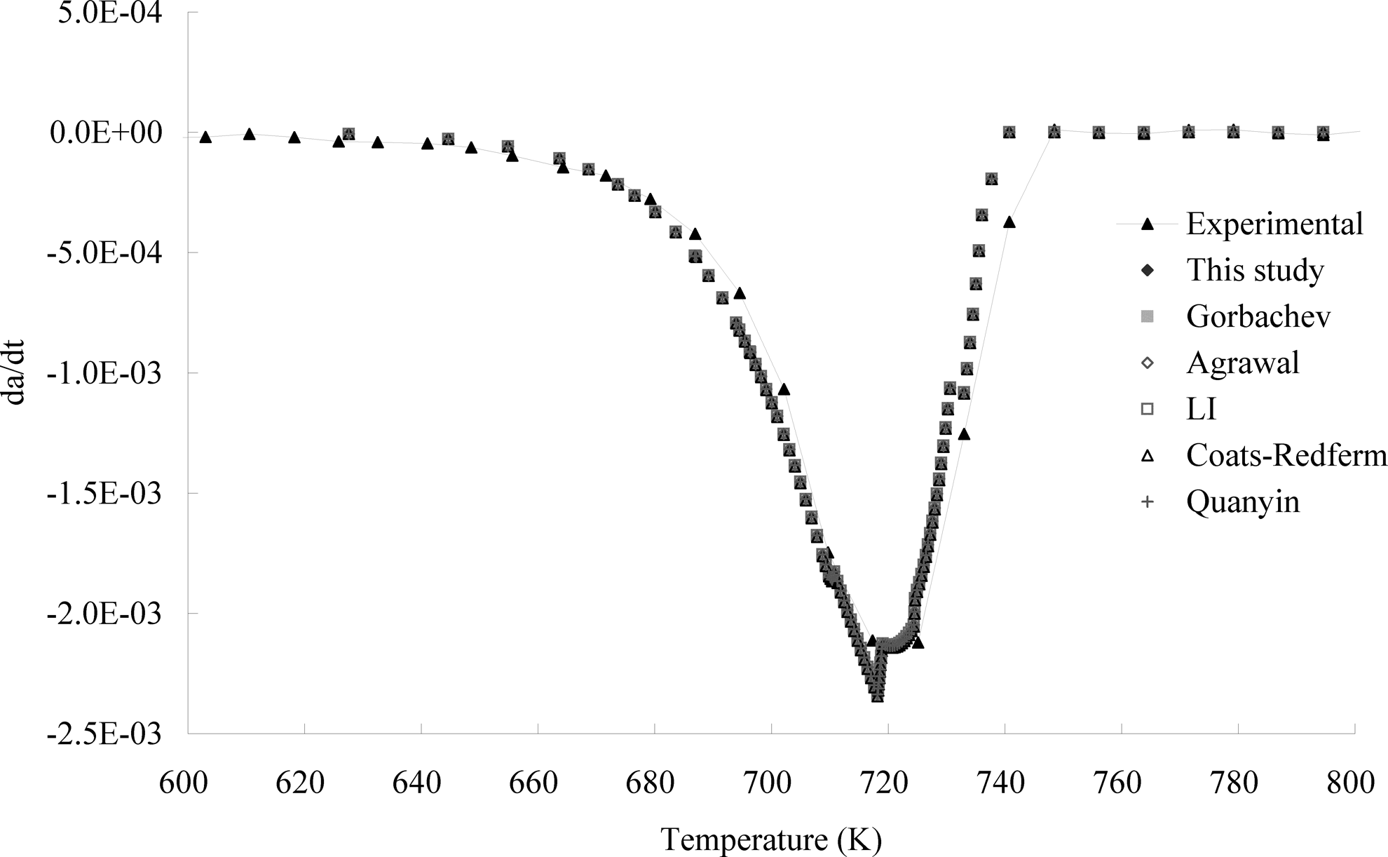
Comparison of the experimental and the simulated DTG curves of polypropylene.

FIG. 7.

The linearity between experimental and simulated DTG data.

FIG. 8.

The results of the coefficient of determination (r²).

Table 3.

The Results of m and A and the Coefficient of Determination, r ²

	This study	Gorbachev	Agrawal	LI	Coats-Redfern	Quanyin
A	6.037×10¹⁴	6.042×10¹⁴	6.040×10¹⁴	6.036×10¹⁴	6.059×10¹⁴	6.039×10¹⁴
m	1.2196	1.2196	1.2196	1.2196	1.2198	1.2196
r²	0.9859	0.9859	0.9859	0.9859	0.9859	0.9859

Evaluation of accuracy

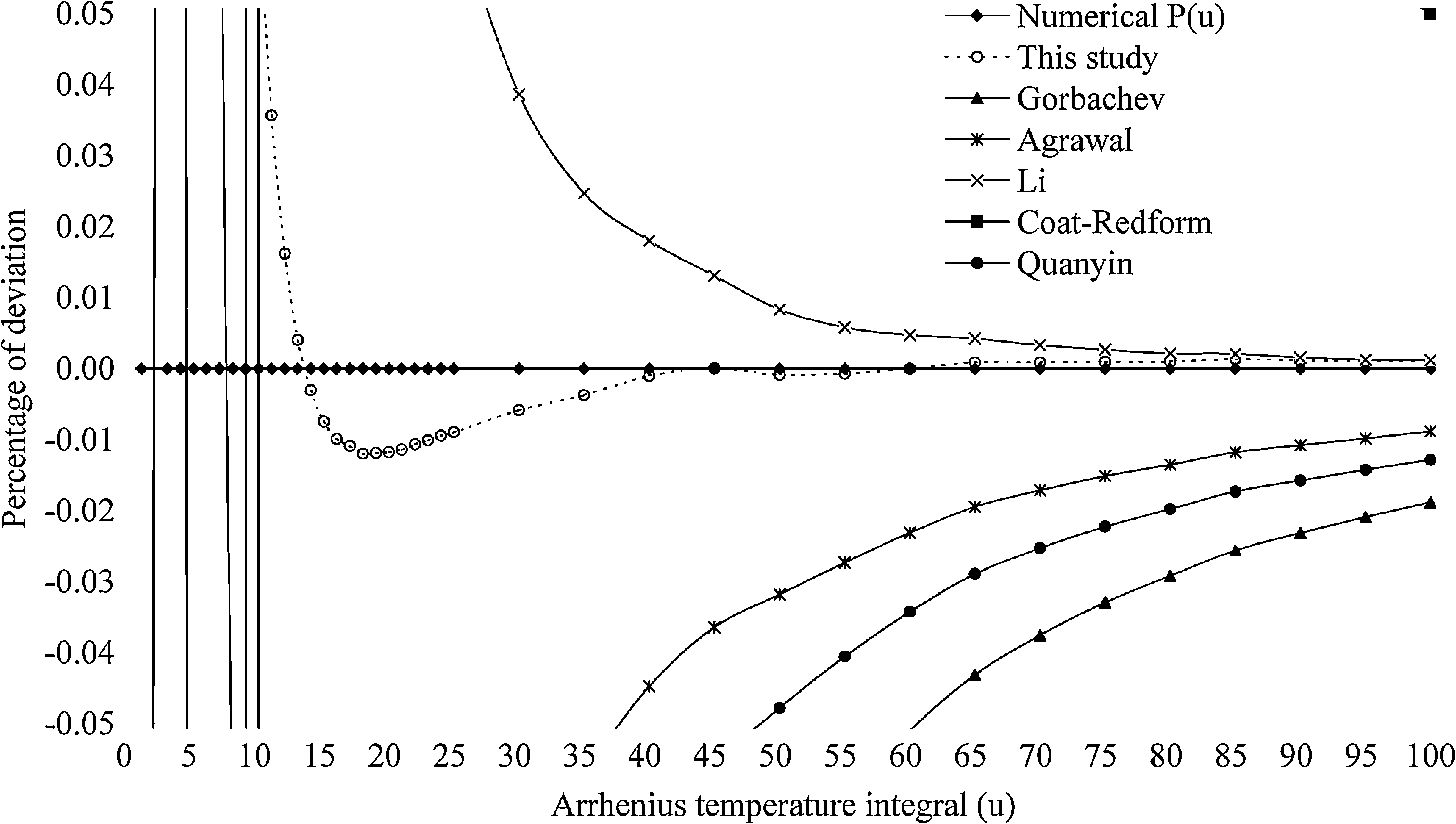
The percentage of deviation from the numerical results of p(u) at different values of u is shown in Table 4 and Fig. 9. Agrawal (1992) has noted that a deviation of <0.1% is desirable for reactions of interest in thermal analysis, although deviations of <1% may be acceptable. Table 5 shows the accuracies of some of the integral approximations. The deviations of the Coats-Redfern equation are >0.1% for u<80. The deviations of the Gorbachev equation are<0.1% for u> 50. The Li equation deviates by <0.1% for u>24 and by <0.01% for u>55. The Agrawal equation deviates by <0.015% for u>85. The Quanyin equation deviates by <0.1% for u>40. The deviations of the new equation proposed in this study are <0.01% for u>35 and by <0.001% for u>70 and the interval of 14 to 15.

FIG. 9.

Comparision of the percentage of deviation from numerical results of the p(u) at different u.

Table 4.

Percentage of Deviation from Numerical Result of p(u) Function for Some Arrhenius Integral Approximations

u	Coats-Redfern	Gorbachev	Li	Agrawal	Quanyin	This study
3	309.67117	−17.42102	−50.45261	−38.06577	−31.18418	−28.64686
4	64.97760	−6.43226	55.94624	16.95968	6.32698	12.43855
5	32.53868	−4.55319	14.53617	4.12379	0.47032	3.50470
6	20.28545	−3.40263	6.76552	1.42724	−0.56153	1.46715
7	13.95791	−2.64358	3.84685	0.49695	−0.78326	0.71761
8	10.21525	−2.11524	2.43754	0.10941	−0.79248	0.37989
9	7.80727	−1.73245	1.65609	−0.06690	−0.73985	0.20879
10	6.16364	−1.44573	1.18238	−0.14896	−0.67174	0.11555
11	4.99075	−1.22479	0.87681	−0.18505	−0.60357	0.06261
12	4.12404	−1.05128	0.66957	−0.19827	−0.54124	0.03120
13	3.46529	−0.91252	0.52353	−0.19966	−0.48603	0.01209
14	2.95281	−0.79990	0.41728	−0.19502	−0.43785	0.00020
15	2.54626	−0.70663	0.33856	−0.18677	−0.39537	−0.00666
16	2.21828	−0.62898	0.27852	−0.17729	−0.35846	−0.01085
17	1.94986	−0.56338	0.23211	−0.16722	−0.32606	−0.01310
18	1.72739	−0.50732	0.19581	−0.15699	−0.29742	−0.01397
19	1.54093	−0.45999	0.16605	−0.14795	−0.27300	−0.01492
20	1.38312	−0.41843	0.14259	−0.13871	−0.25079	−0.01468
21	1.24837	−0.38257	0.12311	−0.13037	−0.23140	−0.01447
22	1.13240	−0.35113	0.10703	−0.12257	−0.21412	−0.01404
23	1.03187	−0.32313	0.09393	−0.11503	−0.19838	−0.01319
24	0.94416	−0.29862	0.08265	−0.10835	−0.18454	−0.01258
25	0.86717	−0.27667	0.07323	−0.10203	−0.17196	−0.01181
30	0.79923	−0.25727	0.06500	−0.09639	−0.16080	−0.01125
35	0.55515	−0.18469	0.03861	−0.07317	−0.11781	−0.00788
40	0.40793	−0.13914	0.02470	−0.05729	−0.09005	−0.00554
45	0.31236	−0.10736	0.01798	−0.04473	−0.06979	−0.00264
50	0.24682	−0.08588	0.01309	−0.03642	−0.05621	−0.00146
55	0.19994	−0.07182	0.00832	−0.03176	−0.04779	−0.00223
60	0.16524	−0.06038	0.00582	−0.02729	−0.04053	−0.00199
65	0.13886	−0.05092	0.00470	−0.02312	−0.03424	−0.00118
70	0.11832	−0.04313	0.00425	−0.01944	−0.02892	−0.00023
75	0.10202	−0.03755	0.00330	−0.01713	−0.02530	−0.00015
80	0.08888	−0.03292	0.00266	−0.01514	−0.02225	−0.00002
85	0.07811	−0.02915	0.00212	−0.01351	−0.01977	0.00003
90	0.06920	−0.02562	0.00208	−0.01177	−0.01731	0.00044
95	0.06172	−0.02313	0.00157	−0.01078	−0.01572	0.00030
100	0.05540	−0.02090	0.00128	−0.00981	−0.01425	0.00028

Table 5.

Ranges of u in Which the Relative Deviation of p(u) Is Lower Than the Indicated Values

	Deviation from numerical p(u)
Authors	<1%	<0.1%	<0.015%	<0.010%	<0.001%
Coats-Redfern	u≥24	u≥80	—	—	—
Gorbachev	u≥13	u≥50	—	—	—
Li	u≥11	u≥23	u≥50	u≥55	—
Agrawal	u≥9	u≥30	u≥85	u≥100	—
Quanyin	u≥5	u≥40	u≥100	—	—
This study	u≥7	u≥11	u≥13	u≥35	u≥70 and 14≤u≤15

Conclusion

In this study, we reviewed several approximate solutions of the Arrhenius temperature integral and found them all to be special cases of the more generic form \documentclass{aastex}\usepackage{amsbsy}\usepackage{amsfonts}\usepackage{amssymb}\usepackage{bm}\usepackage{mathrsfs}\usepackage{pifont}\usepackage{stmaryrd}\usepackage{textcomp}\usepackage{portland, xspace}\usepackage{amsmath, amsxtra}\pagestyle{empty}\DeclareMathSizes{10}{9}{7}{6}\begin{document} $$p (u) = \displaystyle \frac {e^{- u}} {u^2} \frac {1 - \frac {2} {u}} {\left(1 - \frac {\lambda} {u^2} \right)}$$ \end{document} with slight differences in the λ value. Using a rigorous numerical treatment for different values of u, we came to realize that λ is linearly proportional to ln(u) and can be represented as λ=a ln(u)+b, where a and b are equal to 0.33 and 4.48, respectively.

The numerical process can be performed using the Solver algorithm in MS Excel. The results of comparisons of our model with previous models can be seen in Fig. 9 and Table 4. The new formula shows a clear edge over previous models for u in the range of 10≤u≤100, which also covers the range 15≤u≤55, where most thermal decomposition reactions take place.

To prove the applicability of the new approximation of p(u), a polymer material, polypropylene, was used to conduct the TGA experiments. Using the master plot model, the reaction model was found. Figures 6 and 7 show that the simulated values obtained from the new approximation equation fit the experimental data as well as the values obtained from other approximation equations.

The formula proposed in this paper was not obtained from any approximating infinite series. It was obtained from numerical results calculated by computer. The numerical process is reliable and highly accurate. The resultant approximate solution to the Arrhenius temperature integral has been proven to be a viable alternative for evaluating kinetic parameters of nonisothermal TGA of, for example, the pyrolysis of polymeric waste and biomass fuel.

Footnotes

Author Disclosure Statement

No competing financial interests exist.

References

Agrawal

R.K.

1987. A new equation for modeling nonisothermalreactions. J. Therm. Anal. Calorim., 32:149.

Billo

E.J.

2007. Excel for Scientists and Engineers: Numerical Methods. Hoboken, NJ: Wiley-Interscience.

Brems

et al. 2011a. Polymeric cracking of waste polyethylene terephthalate to chemicals and energy. J. Air Waste Manag. Assoc., 61:721.

Brems

et al. 2011b. Thermogravimetric pyrolysis of waste polyethylene-terephthalate and polystyrene: A critical assessment of kinetics modelling. Resour. Conserv. Recy., 55:772.

Butterman

H.C.

, Castaldi

M.J.

2009. Syngas production via CO₂ enhanced gasification of biomass fuels. Environ. Eng. Sci., 26:703.

Butterman

H.C.

, Castaldi

M.J.

2010. Biomass to fuels: Impact of reaction medium and heating rate. Environ. Eng. Sci., 27:539.

Coats

A.W.

, Redfern

J.P.

1964. Kinetic parameters from thermogravimetric data. Nature, 201:68.

Flynn

J.H.

1997. The “temperature integral’'—Its use and abuse. Thermochim. Acta, 300:83.

Gorbachev

V. M.

1977. Exponential-temperature integral in anisothermal kinetics. Zh. Fiz. Khim., 51:2245.

10.

Gotor Francisco

, Criado

J.M.

, Malek

, Koga

2000. Kinetic analysis of solid-state reactions: The universality of master plots for analyzing isothermal and nonisothermal experiments. J. Phys. Chem. A, 104:10777.

11.

Gyulai

, Greenhow

E.J.

1974. A new integral method for the kinetic analysis of thermogravimetric data. J. Therm. Anal. Calorim., 6:279.

12.

Heal

G.R.

1999. Evaluation of the integral of the Arrhenius function by a series of Chebyshev polynomials—Use in the analysis of non-isothermal kinetics. Thermochim. Acta, 340–34169.

13.

Kujirai

, Akahira

1925. Effect of temperature on the deterioration of fibrous insulating materials. Papers Inst. Phys. Chem. Res. (Tokyo), 2:223.

14.

C.-H.

1985. An integral approximation formula for kinetic analysis of nonisothermal TGA data. Aiche J., 31:1036.

15.

Quanyin

, Su

1995. New approximations of the temperature integral for nonisothermal kinetics. J. Therm. Anal., 44:1147.

16.

Rainville

E.D.

1960. Special Functions. New York: Macmillan.

17.

Rodríguez-Barroso

E.A.

2009. Thermal gravimetry analysis assessed as an alternative method for characterization of sediment contamination. Environ. Engin. Sci., 26:279.

18.

Stephen

2003. The Mathematica Book, 5th. Champaign, IL: Wolfram Media, Inc.

19.

Tai

H.-S.

, Hsu

C. H.

2010. A kinetic analysis of thermal degradation of polypropylene using a modified Gompertz model. J. Hazard. Toxic Radioact. Waste 11 Dec 2010[Epub ahead of print]10.1061/(asce)hz.2153-5515.0000095.

20.

Van de Velden

et al. 2008. Modeling CFB biomass pyrolysis reactors. Biomass Bioenerg., 32:128.

21.

Van de Velden

et al. 2010. Fundamentals, kinetics and endothermicity of the biomass pyrolysis reaction. Renew. Energ., 35:2322.