Two-Stage Inexact-Probabilistic Programming Model for Water Quality Management

Abstract

A two-stage inexact-probabilistic programming (TIPP) method was developed for water quality management in Zhangweinan River Basin, through coupling two-stage stochastic programming with inexact chance-constrained programming. The developed TIPP can handle uncertainties presented as both discrete intervals and probability distributions, and can support the assessment of the reliability of satisfying (or the risk of violating) system's constraints for accomplishing a maximized system benefit. It can also be used for analyzing policy scenarios that are associated with different levels of economic penalties when the promised targets are violated. Interval solutions under different constraint-violation levels have been obtained. They can be used for generating decision alternatives and thus help managers to identify desired policies under various environmental, economic, and system-reliability constraints.

Introduction

Although the “global water crisis” tends to be viewed as a water quantity problem, water quality is increasingly being acknowledged as a central factor in the water crisis (Ongley, 2000). In many developing countries (e.g., China), water quality management is becoming more and more important for their sustainable development, due to serious water pollution and increasing demand for clean water. Previously, a large number of mathematical techniques were developed for water quality management to analyze the relevant information, simulate the related processes, evaluate the resulting impacts, and generate sound decision alternatives (Huang, 1996; Li and Huang, 2009; Lv et al., 2010). Simulation-based optimization models were commonly used for optimal decision making in a river system, where water quality simulation model was incorporated within optimization model to provide effective compromise solutions acceptable to both pollution control agency (PCA) and wastewater dischargers (Burn and McBean, 1987; Chan, 1994; Karmakar and Mujumdar, 2006; Ping et al., 2010; Zhao et al., 2011). However, in water quality management problems, various uncertainties exist in a number of system components as well as their interrelationships, such as random nature of input parameters (e.g., stream flow, discharge rate, and temperature) and imprecision or fuzziness associated with setting up water quality standards and goals of both the PCA and wastewater dischargers. This creates difficulties in modeling water quality management problems.

Two-stage stochastic programming (TSP) is effective for problems where an analysis of policy scenarios is desired and the related data are random in nature (Li et al., 2011). In TSP, a decision is first undertaken before values of random variables are known; then, after the random events have happened and their values are known, a second-stage decision can be made in order to minimize “penalties” that may appear due to any infeasibility (Ruszczynski and Swietanowski, 1997; Huang and Loucks, 2000). However, TSP is incapable of accounting for the risk of violating uncertain system constraints and its economic implications. In a real-world water quality management problem, randomness that may result in risk of constraint violation also needs to be reflected. For example, the uncertainties in water quality standards can be understood as satisfying the relevant standards with a level of probability, which represents the admissible risk of violating the uncertain water quality requirements. Chance-constrained programming (CCP) method can provide information on the tradeoffs among the objective function value, tolerance values of the constraints, and the prescribed level of probability, which could be valuable to policy makers and wastewater dischargers (Qin and Huang, 2009). However, traditional CCP is effective in reflecting probability distributions of the constraints' right hand sides but not so much for independent uncertainties of the left hand–side coefficients in each constraint or the objective function; moreover, the quality of many uncertainties is often not satisfactory enough to be presented as probability distributions (Li et al., 2007). A number of researchers proposed inexact CCP models through introduction of interval-parameter programming technique into the CCP framework for river water quality management (Xie et al., 2011).

The objective of this study is to develop a two-stage inexact-probabilistic programming (TIPP) model through coupling TSP with inexact CCP for planning water quality management. TIPP can handle uncertainties in the model's left hand sides and objective function presented as intervals and those in the model's right hand sides as probability distributions. It can also help examine the risk of violating river-quality constraints under uncertainty, and thus quantify the cost of violating the constraints under varied risk levels. The TIPP is applied to Zhangweinan River Basin, where a water quality simulation model is incorporated within the proposed TIPP framework, such that dynamic interactions between pollutant loading and water quality can be effectively reflected under uncertainties. The results can be used for generating a number of decision alternatives under various system conditions, and thus helping managers to identify desired water quality management policies.

Methodology

When uncertainties are expressed as probability distributions and decisions need to be made periodically over time, the problem can be formulated as a TSP model. In TSP, decision variables are divided into two subsets: those that must be determined before the realizations of random variables are known and those (recourse variables) that are determined after the realized values of the random variables are available (Li et al., 2007). A general TSP model can be formulated as follows (Birge and Louveaux, 1997): \documentclass{aastex}\usepackage{amsbsy}\usepackage{amsfonts}\usepackage{amssymb}\usepackage{bm}\usepackage{mathrsfs}\usepackage{pifont}\usepackage{stmaryrd}\usepackage{textcomp}\usepackage{portland, xspace}\usepackage{amsmath, amsxtra}\pagestyle{empty}\DeclareMathSizes{10}{9}{7}{6}\begin{document} \begin{align*} z = \max \ C^T X - E_{\omega \in \Omega} \ [Q (X, \omega)] \tag{1{\rm a}} \end{align*} \end{document}

with \documentclass{aastex}\usepackage{amsbsy}\usepackage{amsfonts}\usepackage{amssymb}\usepackage{bm}\usepackage{mathrsfs}\usepackage{pifont}\usepackage{stmaryrd}\usepackage{textcomp}\usepackage{portland, xspace}\usepackage{amsmath, amsxtra}\pagestyle{empty}\DeclareMathSizes{10}{9}{7}{6}\begin{document} \begin{align*} Q (x, \omega) = \min f (\omega)^T y \end{align*} \end{document}

where \documentclass{aastex}\usepackage{amsbsy}\usepackage{amsfonts}\usepackage{amssymb}\usepackage{bm}\usepackage{mathrsfs}\usepackage{pifont}\usepackage{stmaryrd}\usepackage{textcomp}\usepackage{portland, xspace}\usepackage{amsmath, amsxtra}\pagestyle{empty}\DeclareMathSizes{10}{9}{7}{6}\begin{document} $$X \in R^{n_1},C \in R^{n_1}$$ \end{document} , and \documentclass{aastex}\usepackage{amsbsy}\usepackage{amsfonts}\usepackage{amssymb}\usepackage{bm}\usepackage{mathrsfs}\usepackage{pifont}\usepackage{stmaryrd}\usepackage{textcomp}\usepackage{portland, xspace}\usepackage{amsmath, amsxtra}\pagestyle{empty}\DeclareMathSizes{10}{9}{7}{6}\begin{document} $$Y \in R^{n_2}$$ \end{document} . Here, ω is a random variable from space (Ω, F, P) with Ω⊆R^K, \documentclass{aastex}\usepackage{amsbsy}\usepackage{amsfonts}\usepackage{amssymb}\usepackage{bm}\usepackage{mathrsfs}\usepackage{pifont}\usepackage{stmaryrd}\usepackage{textcomp}\usepackage{portland, xspace}\usepackage{amsmath, amsxtra}\pagestyle{empty}\DeclareMathSizes{10}{9}{7}{6}\begin{document} $$f: \Omega \rightarrow R^{n_2}, h: \Omega \rightarrow R^{m_2}, D: \Omega \rightarrow R^{m_2 \times n_2}, \ {\rm and} \ T: \Omega \rightarrow R^{m_2 \times n_1}$$ \end{document} . By letting random variables (i.e., ω) take discrete values w_h with probability levels \documentclass{aastex}\usepackage{amsbsy}\usepackage{amsfonts}\usepackage{amssymb}\usepackage{bm}\usepackage{mathrsfs}\usepackage{pifont}\usepackage{stmaryrd}\usepackage{textcomp}\usepackage{portland, xspace}\usepackage{amsmath, amsxtra}\pagestyle{empty}\DeclareMathSizes{10}{9}{7}{6}\begin{document} $$p_h (h = 1, 2, \ldots, v$$ \end{document} and \documentclass{aastex}\usepackage{amsbsy}\usepackage{amsfonts}\usepackage{amssymb}\usepackage{bm}\usepackage{mathrsfs}\usepackage{pifont}\usepackage{stmaryrd}\usepackage{textcomp}\usepackage{portland, xspace}\usepackage{amsmath, amsxtra}\pagestyle{empty}\DeclareMathSizes{10}{9}{7}{6}\begin{document} $$\sum p_h = 1)$$ \end{document} , the above TSP can be equivalently formulated as a linear programming model (Huang and Loucks, 2000). In a real-world management problem, randomness in other right hand–side parameters also needs to be reflected. For example, the water quality standards maybe fixed with a level of probability, that is, \documentclass{aastex}\usepackage{amsbsy}\usepackage{amsfonts}\usepackage{amssymb}\usepackage{bm}\usepackage{mathrsfs}\usepackage{pifont}\usepackage{stmaryrd}\usepackage{textcomp}\usepackage{portland, xspace}\usepackage{amsmath, amsxtra}\pagestyle{empty}\DeclareMathSizes{10}{9}{7}{6}\begin{document} $$q_s \in [0, 1]$$ \end{document} , which represents the admissible risk of violating the uncertain standard constraint. The CCP method can be used for dealing with this type of uncertainty. In CCP, it is required that the constraints be satisfied under given probabilities. A general CCP formulation can be expressed as (Charnes et al., 1972; Huang, 1998): \documentclass{aastex}\usepackage{amsbsy}\usepackage{amsfonts}\usepackage{amssymb}\usepackage{bm}\usepackage{mathrsfs}\usepackage{pifont}\usepackage{stmaryrd}\usepackage{textcomp}\usepackage{portland, xspace}\usepackage{amsmath, amsxtra}\pagestyle{empty}\DeclareMathSizes{10}{9}{7}{6}\begin{document} \begin{align*} {\rm Max} \ c^T x \tag{2{\rm a}} \end{align*} \end{document}

Model (2) can be converted into deterministic versions through (i) fixing a certain level of probability q_s for uncertain constraint s, and (ii) imposing the condition that the constraint should be satisfied with at least a probability level of 1−q_s (Huang, 1998). The problem with Equation (2b) is that linear constraints can only reflect the case when the left hand–side coefficients (A) are deterministic. If both left and right hand sides (A and B) are uncertain, the set of feasible constraints may become more complicated; this brings about considerable difficulty to its practical application, particularly for large-scale problems (Huang, 1998). On the other hand, in many real-world situations, the distribution information may hardly be known while only two bounds of each imprecise parameter can be identified as intervals. Therefore, for reflecting uncertainties presented as intervals (in A and C), an extended consideration is the introduction of interval-parameter programming technique into the CCP framework. This leads to an inexact chance-constrained programming (ICCP) model as follows: \documentclass{aastex}\usepackage{amsbsy}\usepackage{amsfonts}\usepackage{amssymb}\usepackage{bm}\usepackage{mathrsfs}\usepackage{pifont}\usepackage{stmaryrd}\usepackage{textcomp}\usepackage{portland, xspace}\usepackage{amsmath, amsxtra}\pagestyle{empty}\DeclareMathSizes{10}{9}{7}{6}\begin{document} \begin{align*} {\rm Max} \ f^{\pm} = C^{\pm} X^{\pm} \tag{3{\rm a}} \end{align*} \end{document}

Model (4) can be transformed into two deterministic submodels that correspond to the lower and upper bounds of desired objective function value. This transformation process is based on an interactive algorithm, which is different from the best/worst case analysis (Huang, 1998). Interval solutions associated with varying levels of constraint-violation risk can then be obtained by solving the two submodels sequentially. Submodel corresponding to upper-bound objective value (f⁺) can be firstly formulated as follows (assume that B^±>0 and f ^±>0): \documentclass{aastex}\usepackage{amsbsy}\usepackage{amsfonts}\usepackage{amssymb}\usepackage{bm}\usepackage{mathrsfs}\usepackage{pifont}\usepackage{stmaryrd}\usepackage{textcomp}\usepackage{portland, xspace}\usepackage{amsmath, amsxtra}\pagestyle{empty}\DeclareMathSizes{10}{9}{7}{6}\begin{document} \begin{align*} &{\rm Max} \ f^+ = \sum_{j = 1}^{k_1} c_j^+ x_j^+ + \sum_{j = k_1 + 1}^{n_1} c_j^+ x_j^- \\& \quad + \sum_{j = 1}^{k_2} \sum_{h = 1}^v p {}_{jh} d_j^- y_{jh}^- + \sum_{j = k_2 + 1}^{n_2} \sum_{h = 1}^v p {}_{jh} d_j^- y_{jh}^+ \tag{5{\rm a}} \end{align*} \end{document}

subject to \documentclass{aastex}\usepackage{amsbsy}\usepackage{amsfonts}\usepackage{amssymb}\usepackage{bm}\usepackage{mathrsfs}\usepackage{pifont}\usepackage{stmaryrd}\usepackage{textcomp}\usepackage{portland, xspace}\usepackage{amsmath, amsxtra}\pagestyle{empty}\DeclareMathSizes{10}{9}{7}{6}\begin{document} \begin{align*} \sum_{j = 1}^{k_1} \mid a_{r_j} \mid^- \ {\rm Sign} (a_{rj}^-) x_j^+ + \sum_{j = k_1 + 1}^{n_1} \mid a_{rj} \mid^+ \ {\rm Sign} (a_{rj}^+) x_j^- \leq b_r^+, \forall r \tag{5{\rm b}} \end{align*} \end{document} \documentclass{aastex}\usepackage{amsbsy}\usepackage{amsfonts}\usepackage{amssymb}\usepackage{bm}\usepackage{mathrsfs}\usepackage{pifont}\usepackage{stmaryrd}\usepackage{textcomp}\usepackage{portland, xspace}\usepackage{amsmath, amsxtra}\pagestyle{empty}\DeclareMathSizes{10}{9}{7}{6}\begin{document} \begin{align*} &\sum_{j = 1}^{k_1} \mid a_{tj} \mid^- \ {\rm Sign} (a_{tj}^-) x_j^+ + \sum_{j = k_1 + 1}^{n_1} \mid a_{tj} \mid^+ \ {\rm Sign} (a_{tj}^+) x_j^- \\&\quad + \sum_{j = 1}^{k_2} \mid a_{tj}^{\prime} \mid^+ \ {\rm Sign} (a_{tj}^{\prime +}) y_{jh}^- \\&\quad + \sum_{j = k_2 + 1}^{n_2} \mid a_{tj}^{\prime} \mid^- {\rm Sign} (a_{tj}^{\prime -}) y_{jh}^+ \leq w_h^+, \forall t, h \tag{5{\rm c}} \end{align*} \end{document} \documentclass{aastex}\usepackage{amsbsy}\usepackage{amsfonts}\usepackage{amssymb}\usepackage{bm}\usepackage{mathrsfs}\usepackage{pifont}\usepackage{stmaryrd}\usepackage{textcomp}\usepackage{portland, xspace}\usepackage{amsmath, amsxtra}\pagestyle{empty}\DeclareMathSizes{10}{9}{7}{6}\begin{document} \begin{align*} &\sum_{j = 1}^{k_1} \mid a_{sj} \mid^- \ {\rm Sign} (a_{sj}^-) x_j^+ + \sum_{j = k_1 + 1}^{n_1} \mid a_{sj} \mid^+ \ {\rm Sign} (a_{sj}^+) x_j^- \\&\quad + \sum_{j = 1}^{k_2} \mid a_{sj}^{\prime} \mid^+ \ {\rm Sign} (a_{sj}^{\prime +}) y_{jh}^- \\ &\quad + \sum_{j = k_2 + 1}^{n_2} \mid a_{sj}^{\prime} \mid^- \ {\rm Sign} (a_{sj}^{\prime -}) y_{jh}^+ \leq (b_s^+)^{(q_s)}, \forall s, h \tag{5{\rm d}} \end{align*} \end{document} \documentclass{aastex}\usepackage{amsbsy}\usepackage{amsfonts}\usepackage{amssymb}\usepackage{bm}\usepackage{mathrsfs}\usepackage{pifont}\usepackage{stmaryrd}\usepackage{textcomp}\usepackage{portland, xspace}\usepackage{amsmath, amsxtra}\pagestyle{empty}\DeclareMathSizes{10}{9}{7}{6}\begin{document} \begin{align*} & x_j^+ \geq 0, \ j = 1, \ 2, \cdots, k_1 & (5{\rm e}) \\ & x_j^- \geq 0, \ j = k_1 + 1, \ k_1 + 2, \cdots, n_1 & (5{\rm f}) \\ & y_{jh}^- \geq 0, \ \forall h; \ j = 1, \ 2, \cdots, k_2 & (5{\rm g}) \\ & y_{jh}^+ \geq 0, \ \forall h; \ j = k_2 + 1, \ k_2 + 2, \cdots, n_2 & (5{\rm h}) \end{align*} \end{document}

where \documentclass{aastex}\usepackage{amsbsy}\usepackage{amsfonts}\usepackage{amssymb}\usepackage{bm}\usepackage{mathrsfs}\usepackage{pifont}\usepackage{stmaryrd}\usepackage{textcomp}\usepackage{portland, xspace}\usepackage{amsmath, amsxtra}\pagestyle{empty}\DeclareMathSizes{10}{9}{7}{6}\begin{document} $$x_j^{\pm}, j = 1, 2, \ldots, k_1$$ \end{document} , are interval variables with positive coefficients in the objective function; \documentclass{aastex}\usepackage{amsbsy}\usepackage{amsfonts}\usepackage{amssymb}\usepackage{bm}\usepackage{mathrsfs}\usepackage{pifont}\usepackage{stmaryrd}\usepackage{textcomp}\usepackage{portland, xspace}\usepackage{amsmath, amsxtra}\pagestyle{empty}\DeclareMathSizes{10}{9}{7}{6}\begin{document} $$x_j^{\pm}, j = k_1 + 1, \ k_1 + 2, \ldots, n_1$$ \end{document} , are interval variables with negative coefficients; \documentclass{aastex}\usepackage{amsbsy}\usepackage{amsfonts}\usepackage{amssymb}\usepackage{bm}\usepackage{mathrsfs}\usepackage{pifont}\usepackage{stmaryrd}\usepackage{textcomp}\usepackage{portland, xspace}\usepackage{amsmath, amsxtra}\pagestyle{empty}\DeclareMathSizes{10}{9}{7}{6}\begin{document} $$y_{jh}^{\pm}, j = 1, 2, \ldots, k_2$$ \end{document} and \documentclass{aastex}\usepackage{amsbsy}\usepackage{amsfonts}\usepackage{amssymb}\usepackage{bm}\usepackage{mathrsfs}\usepackage{pifont}\usepackage{stmaryrd}\usepackage{textcomp}\usepackage{portland, xspace}\usepackage{amsmath, amsxtra}\pagestyle{empty}\DeclareMathSizes{10}{9}{7}{6}\begin{document} $$h = 1, 2, \ldots, v$$ \end{document} are random variables with positive coefficients in the objective function; \documentclass{aastex}\usepackage{amsbsy}\usepackage{amsfonts}\usepackage{amssymb}\usepackage{bm}\usepackage{mathrsfs}\usepackage{pifont}\usepackage{stmaryrd}\usepackage{textcomp}\usepackage{portland, xspace}\usepackage{amsmath, amsxtra}\pagestyle{empty}\DeclareMathSizes{10}{9}{7}{6}\begin{document} $$y_{jh}^{\pm}, j = k_2 + 1, \ k_2 + 2, \ldots, n_2$$ \end{document} and \documentclass{aastex}\usepackage{amsbsy}\usepackage{amsfonts}\usepackage{amssymb}\usepackage{bm}\usepackage{mathrsfs}\usepackage{pifont}\usepackage{stmaryrd}\usepackage{textcomp}\usepackage{portland, xspace}\usepackage{amsmath, amsxtra}\pagestyle{empty}\DeclareMathSizes{10}{9}{7}{6}\begin{document} $$h = 1, 2, \ldots, v$$ \end{document} , are random variables with negative coefficients. Solutions of \documentclass{aastex}\usepackage{amsbsy}\usepackage{amsfonts}\usepackage{amssymb}\usepackage{bm}\usepackage{mathrsfs}\usepackage{pifont}\usepackage{stmaryrd}\usepackage{textcomp}\usepackage{portland, xspace}\usepackage{amsmath, amsxtra}\pagestyle{empty}\DeclareMathSizes{10}{9}{7}{6}\begin{document} $$x_{j{\rm opt}}^- (j = 1, 2, \ldots, k_1), \ x_{j{\rm opt}}^+ (j = k_1 + 1, \ k_1 + 2, \ldots, n_1), \ \ y_{jh{\rm opt}}^- (j = 1, 2, \ldots, k_2)$$ \end{document} , and \documentclass{aastex}\usepackage{amsbsy}\usepackage{amsfonts}\usepackage{amssymb}\usepackage{bm}\usepackage{mathrsfs}\usepackage{pifont}\usepackage{stmaryrd}\usepackage{textcomp}\usepackage{portland, xspace}\usepackage{amsmath, amsxtra}\pagestyle{empty}\DeclareMathSizes{10}{9}{7}{6}\begin{document} $$y_{jh {\rm opt}}^+ (j = k_2 + 1, k_2 + 2, \ldots, n_2)$$ \end{document} can be obtained through Submodel (5). Based on the solutions just outlined, the second submodel for f⁻ can be formulated as follows: \documentclass{aastex}\usepackage{amsbsy}\usepackage{amsfonts}\usepackage{amssymb}\usepackage{bm}\usepackage{mathrsfs}\usepackage{pifont}\usepackage{stmaryrd}\usepackage{textcomp}\usepackage{portland, xspace}\usepackage{amsmath, amsxtra}\pagestyle{empty}\DeclareMathSizes{10}{9}{7}{6}\begin{document} \begin{align*} {\rm Max} \ f^- &= \sum_{j = 1}^{k_1} c_j^- x_j^- + \sum_{j = k_1 + 1}^{n_1} c_j^- x_j^+ \\&\quad+ \sum_{j = 1}^{k_2} \sum_{h = 1}^v p {}_{jh} d_j^+ y_{jh}^+ + \sum_{j = k_2 + 1}^{n_2} \sum_{h = 1}^v p {}_{jh} d_j^+ y_{jh}^- \tag{6{\rm a}} \end{align*} \end{document}

subject to \documentclass{aastex}\usepackage{amsbsy}\usepackage{amsfonts}\usepackage{amssymb}\usepackage{bm}\usepackage{mathrsfs}\usepackage{pifont}\usepackage{stmaryrd}\usepackage{textcomp}\usepackage{portland, xspace}\usepackage{amsmath, amsxtra}\pagestyle{empty}\DeclareMathSizes{10}{9}{7}{6}\begin{document} \begin{align*} \sum_{j = 1}^{k_1} \mid a_{r_j} \mid^+ \ {\rm Sign} (a_{rj}^+) x_j^- + \sum_{j = k_1 + 1}^{n_1} \mid a_{rj} \mid^- \ {\rm Sign} (a_{rj}^-) x_j^+ \leq b_r^-, \forall r \tag{6{\rm b}} \end{align*} \end{document} \documentclass{aastex}\usepackage{amsbsy}\usepackage{amsfonts}\usepackage{amssymb}\usepackage{bm}\usepackage{mathrsfs}\usepackage{pifont}\usepackage{stmaryrd}\usepackage{textcomp}\usepackage{portland, xspace}\usepackage{amsmath, amsxtra}\pagestyle{empty}\DeclareMathSizes{10}{9}{7}{6}\begin{document} \begin{align*} &\sum_{j = 1}^{k_1} \mid a_{tj} \mid^+ \ {\rm Sign} (a_{tj}^+) x_j^- + \sum_{j = k_1 + 1}^{n_1} \mid a_{tj} \mid^- \ {\rm Sign} (a_{tj}^-) x_j^+ \\&\quad + \sum_{j = 1}^{k_2} \mid a_{tj}^{\prime} \mid^- \ {\rm Sign} (a_{tj}^{\prime -}) y_{jh}^+ \\ &\quad + \sum_{j = k_2 + 1}^{n_2} \mid a_{tj}^{\prime} \mid^+ \ {\rm Sign} (a_{tj}^{\prime +}) y_{jh}^- \leq w_h^-, \forall t, h \tag{6{\rm c}} \end{align*} \end{document} \documentclass{aastex}\usepackage{amsbsy}\usepackage{amsfonts}\usepackage{amssymb}\usepackage{bm}\usepackage{mathrsfs}\usepackage{pifont}\usepackage{stmaryrd}\usepackage{textcomp}\usepackage{portland, xspace}\usepackage{amsmath, amsxtra}\pagestyle{empty}\DeclareMathSizes{10}{9}{7}{6}\begin{document} \begin{align*} &\sum_{j = 1}^{k_1} \mid a_{sj} \mid^+ \ {\rm Sign} (a_{sj}^+) x_j^- + \sum_{j = k_1 + 1}^{n_1} \mid a_{sj} \mid^- \ {\rm Sign} (a_{sj}^-) x_j^+ \\&\quad + \sum_{j = 1}^{k_2} \mid a_{sj}^{\prime} \mid^- \ {\rm Sign} (a_{sj}^{\prime -}) y_{jh}^+ \\ &\quad + \sum_{j = k_2 + 1}^{n_2} \mid a_{sj}^{\prime} \mid^+ \ {\rm Sign} (a_{sj}^{\prime +}) y_{jh}^- \leq (b_s^-)^{(q_s)}, \forall s, h \tag{6{\rm d}} \end{align*} \end{document} \documentclass{aastex}\usepackage{amsbsy}\usepackage{amsfonts}\usepackage{amssymb}\usepackage{bm}\usepackage{mathrsfs}\usepackage{pifont}\usepackage{stmaryrd}\usepackage{textcomp}\usepackage{portland, xspace}\usepackage{amsmath, amsxtra}\pagestyle{empty}\DeclareMathSizes{10}{9}{7}{6}\begin{document} \begin{align*} & 0 \leq x_j^- \leq x_{j {\rm opt}}^+, \ j = 1, \ 2, \cdots, k_1 & (6{\rm e}) \\ & x_j^+ \geq x_{j{\rm opt}}^-, j = k_1 + 1, \ k_1 + 2, \cdots, n_1 & (6{\rm f}) \\ & y_{jh}^+ \geq y_{jh{\rm opt}}^-, \ \forall h; \ j = 1, \ 2, \cdots, k_2 & (6{\rm g}) \\ & 0 \leq y_{jh}^- \leq y_{jh {\rm opt}}^+, \ \forall h; \ j = k_2 + 1, \ k_2 + 2, \cdots, n_2 & (6{\rm h}) \end{align*} \end{document}

Solutions of \documentclass{aastex}\usepackage{amsbsy}\usepackage{amsfonts}\usepackage{amssymb}\usepackage{bm}\usepackage{mathrsfs}\usepackage{pifont}\usepackage{stmaryrd}\usepackage{textcomp}\usepackage{portland, xspace}\usepackage{amsmath, amsxtra}\pagestyle{empty}\DeclareMathSizes{10}{9}{7}{6}\begin{document} $$x_{j {\rm opt}}^+ (j = 1, 2, \ldots, k_1), \ x_{j {\rm opt}}^- (\,j = k_1 + 1, k_1 + 2, \ldots, n_1), \ y_{jh{\rm opt}}^+ (j = 1, 2, \ldots, k_2)$$ \end{document} , and \documentclass{aastex}\usepackage{amsbsy}\usepackage{amsfonts}\usepackage{amssymb}\usepackage{bm}\usepackage{mathrsfs}\usepackage{pifont}\usepackage{stmaryrd}\usepackage{textcomp}\usepackage{portland, xspace}\usepackage{amsmath, amsxtra}\pagestyle{empty}\DeclareMathSizes{10}{9}{7}{6}\begin{document} $$y_{jh{\rm opt}}^- (j = k_2 + 1, k_2 + 2, \ldots, n_2)$$ \end{document} can be obtained through Submodel (6). Through integrating solutions of Submodels (5) and (6), interval solution for Model (4) under a set of \documentclass{aastex}\usepackage{amsbsy}\usepackage{amsfonts}\usepackage{amssymb}\usepackage{bm}\usepackage{mathrsfs}\usepackage{pifont}\usepackage{stmaryrd}\usepackage{textcomp}\usepackage{portland, xspace}\usepackage{amsmath, amsxtra}\pagestyle{empty}\DeclareMathSizes{10}{9}{7}{6}\begin{document} $$q_s (s = 1, 2, \ldots, m_3)$$ \end{document} levels can be obtained.

Case Study

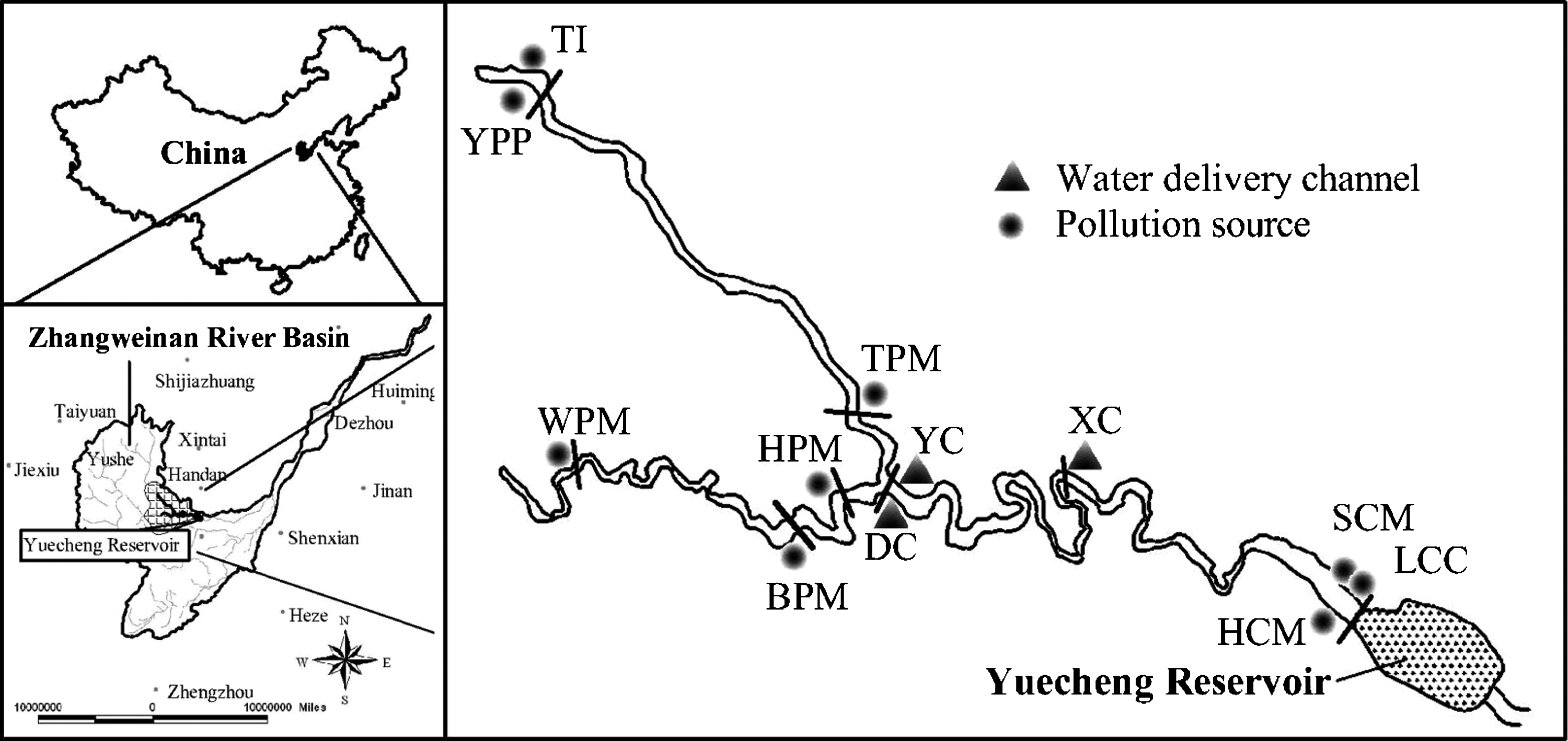
A case study of water quality management for Yuecheng Reservoir that is located in Zhangweinan River Basin in North China will be provided. The reservoir is one of the key drinking water sources in this basin, and responsible for the municipal, industrial, and agricultural water supply of two cities (i.e., Anyang and Handan). Therefore, the water quality management for this reservoir and its upstream river system is of significant importance, as presented in Fig. 1. The average inflow of the reservoir is 0.76×10⁹ m³ from 1962 to 2007, with the maximum inflow of 4.82×10⁹ m³ and the minimum inflow of 0.03×10⁹ m³.* The upstream river system of Yuecheng Reservoir consists of two tributaries, Qingzhang River and Zhuzhang River, which converge into Zhang River and then flow into the reservoir. Nine main wastewater dischargers exist along the river.†^,‡ Three diversion canals scattered in the river system to supply water to agricultural irrigation in this basin.‡

FIG. 1.

Schematic diagram of the study system. Inflow biochemical oxygen demand (BOD) and dissolved-oxygen (DO) concentrations are 3.1 and 5.8 mg/L, respectively, in tributary 1, while 3.2 and 5.6 mg/L in tributary 2; the saturated oxygen concentration is 10 mg/L when the stream temperature is about 14°C (average year temperature in the basin); BOD deoxygenation rate (k_d) and reaeration rate (k_a) are 0.60 day⁻¹ and 0.80 day⁻¹, respectively, in the stream, while 0.20 day⁻¹ and 0.10 day⁻¹ in the reservoir; the average flow velocity is 86.4 km/day; the retention time of Yuecheng Reservoir is 2 years. YC, DC, and XC are three diversion canals, which denote Yuejing Canal, Dayuefeng Canal, and Xiaoyuefeng Canal; while TI, YPP, TPM, WPM, BPM, HPM, HCM, SCM, and LCC are nine dischargers, which denote Tianjin Ironworks, Yiwuling Power Plant, Taizhuang Paper Mill, Wangjiazhuang Paper Mill, Baishan Paper Mill, Huanglongkou Paper Mill, Huangsha Coal Mine, Shenjiazhuang Coal Mine, and Liuhe Coal Company.

In recent decades, with the decrease of reservoir's inflows and the increase of wastewater discharges, water quality (in the reservoir and its upstream river system) is deteriorating, particularly in the nonflooding seasons. Chemical oxygen demand (COD) and ammonia nitrogen are two main pollutants. Wastewater discharged into the river was 1.86×10⁶ ton/day, while COD discharged was 0.64×10⁶ ton/day and ammonia nitrogen discharged was 0.07×10⁶ ton/day.‡ Moreover, wastewater discharge is increasing with the local economy development and population growth, and six of the nine sources could not reach wastewater-discharge standard for surface water quality.‡ In addition, with precipitation decreasing and the amount of reservoirs and diversion canals increasing in the upper reaches of the Zhangweinan River, the inflow of Yuecheng Reservoir becomes much less than that in decades ago. For example, the average annual inflow of the reservoir was 1.83×10⁹ m³ from 1962 to 1970, 0.42×10⁹ m³ from 1981 to 1990, and 0.34×10⁹ m³ from 2001 to 2007 (Li et al., 2010).* The water quality of the upper reaches was Class III (for residential and fishery areas) or inferior to this level. Generally, conflicts exist among these competing dischargers due to the desire to expand production scale and the commitment to comply with the environmental standards. To guarantee a good water quality in Yuecheng Reservoir and make effective tradeoffs between economic and environmental objectives, a sound water quality management in the study system is desired.

For the river water, a minimum dissolved-oxygen (DO) level is required for supporting aquatic life and maintaining aerobic condition (USEPA, 1981). The Streeter–Phelps model is used for quantifying water quality constraints related to biochemical oxygen demand (BOD) and DO discharges as well as reflecting deoxygenation and reaeration dynamics in the upstream river of Yuecheng Reservoir, while the one-dimensional mixing lake model is used for simulating the water quality of Yuecheng Reservoir (Streeter and Phelps, 1925). Thus, the BOD load and DO deficit in relation to the m wastewater discharge sources can be predicted as follows (Thomann and Mueller, 1987; Eckenfelder, 2000): \documentclass{aastex}\usepackage{amsbsy}\usepackage{amsfonts}\usepackage{amssymb}\usepackage{bm}\usepackage{mathrsfs}\usepackage{pifont}\usepackage{stmaryrd}\usepackage{textcomp}\usepackage{portland, xspace}\usepackage{amsmath, amsxtra}\pagestyle{empty}\DeclareMathSizes{10}{9}{7}{6}\begin{document} \begin{align*} L_n &= \prod_{j = 1}^n e^{- k_d t_j} L_0 + \prod_{j = 2}^n e^{- k_d t_j} (1 - \eta_1) BOD_1 + \ldots \\& \quad+ e^{- k_d t_n} (1 - \eta_{m - 1}) BOD_{m - 1} + (1 - \eta_m) BOD_m & (7 {\rm a}) \\ D_n &= \frac {k_d} {k_a - k_d} L_{n - 1} (e^{- k_d t_{n - 1}} - e^{- k_a t_{n - 1}}) + D_{n - 1} e^{- k_at_{n - 1}} & (7 {\rm b}) \end{align*} \end{document}

where j is defined as a segmentation of the stream between source j to \documentclass{aastex}\usepackage{amsbsy}\usepackage{amsfonts}\usepackage{amssymb}\usepackage{bm}\usepackage{mathrsfs}\usepackage{pifont}\usepackage{stmaryrd}\usepackage{textcomp}\usepackage{portland, xspace}\usepackage{amsmath, amsxtra}\pagestyle{empty}\DeclareMathSizes{10}{9}{7}{6}\begin{document} $$j + 1 (j = 1, 2, \ldots, n)$$ \end{document} ; L₀ is the initial BOD in the stream immediately after discharge (mg/L); L_n−₁ and L_n are the respective BOD loads in the river at the beginnings of reaches n−1 and n; k_d is the first-order deoxygenation rate constant (day⁻¹); k_a is the first-order reaeration rate constant (day⁻¹); D_n₋₁ and D_n are the oxygen deficits at the beginnings of reaches n−1 and n, respectively; t_j is the length of reach j expressed in time units; i denotes wastewater discharge source, and i=1, 2, …, m; η_i is the wastewater treatment efficiency at discharge source i; BOD_i is the total amount of BOD to be disposed of at source i (kg/day).

Then, the basic mass balance equation of BOD and DO in one-dimensional mixing lake model can be expressed as follows (Thomann and Mueller, 1987): \documentclass{aastex}\usepackage{amsbsy}\usepackage{amsfonts}\usepackage{amssymb}\usepackage{bm}\usepackage{mathrsfs}\usepackage{pifont}\usepackage{stmaryrd}\usepackage{textcomp}\usepackage{portland, xspace}\usepackage{amsmath, amsxtra}\pagestyle{empty}\DeclareMathSizes{10}{9}{7}{6}\begin{document} \begin{align*} \frac {dVL} {dt} &= QL_{in} - QL - k_d^{\prime} VL & (8 {\rm a}) \\ \frac {dVO} {dt} & = QO - QO_{in} - k_a^{\prime} V (O_s - O) + k_d^{\prime} VL & (8 {\rm b}) \end{align*} \end{document}

where V is the volume of the lake (m³); L is the concentration of BOD in the lake (mg/L); Q is the lake flow (m³/day); L_in is the inflow concentration of BOD (mg/L); \documentclass{aastex}\usepackage{amsbsy}\usepackage{amsfonts}\usepackage{amssymb}\usepackage{bm}\usepackage{mathrsfs}\usepackage{pifont}\usepackage{stmaryrd}\usepackage{textcomp}\usepackage{portland, xspace}\usepackage{amsmath, amsxtra}\pagestyle{empty}\DeclareMathSizes{10}{9}{7}{6}\begin{document} $$k_d^{\prime}$$ \end{document} is the BOD decay rate in the lake (day⁻¹); O is the DO concentration in the lake (mg/L); O_in is the inflow DO concentration (mg/L); \documentclass{aastex}\usepackage{amsbsy}\usepackage{amsfonts}\usepackage{amssymb}\usepackage{bm}\usepackage{mathrsfs}\usepackage{pifont}\usepackage{stmaryrd}\usepackage{textcomp}\usepackage{portland, xspace}\usepackage{amsmath, amsxtra}\pagestyle{empty}\DeclareMathSizes{10}{9}{7}{6}\begin{document} $$k_a^{\prime}$$ \end{document} is the reaeration rate in the lake (day⁻¹). Under steady state conditions, the equilibrium concentrations of BOD and DO are providing as follows: \documentclass{aastex}\usepackage{amsbsy}\usepackage{amsfonts}\usepackage{amssymb}\usepackage{bm}\usepackage{mathrsfs}\usepackage{pifont}\usepackage{stmaryrd}\usepackage{textcomp}\usepackage{portland, xspace}\usepackage{amsmath, amsxtra}\pagestyle{empty}\DeclareMathSizes{10}{9}{7}{6}\begin{document} \begin{align*} & L \approx \frac {L_{in}} {1 + k_d^{\prime} t_d} & (9 {\rm a}) \\ & D \approx \frac {1} {1 + k_a^{\prime} t_d} D_{in} + \frac {k_d^{\prime} t_d} {1 + k_a^{\prime} t_d} \times \frac {L_{in}} {1 + k_d^{\prime} t_d} & (9 {\rm b}) \end{align*} \end{document}

where t_d is the lake retention time (day), which can be calculated by t_d=V/Q. All interest dischargers need to know the targeted pollutant-discharge allowances (i.e., production levels) that they can expect in order to generate appropriate plans for various activities under constraints of water quality criteria. If the targets are too relaxed, high penalties may have to be paid when the allowances are violated (Li and Huang, 2007); conversely, too strict targets may result in opportunity losses with reduced economic benefits. In this study, the volume and strength of industrial wastewater are defined in terms of units of production (e.g., gallons of wastewater per ton of pulp produced), and their variations can be estimated through identifying a statistical distribution for each discharge (Eckenfelder, 2000). Consequently, different water quality requirements (i.e., corresponding to different q levels) could result in different production levels of the dischargers. The production levels can be transformed into production loadings by multiplying the amount of pollutants generated by each product unit. By the introduction of the water quality simulation model into the TIPP framework, the study problem can be formulated as follows: \documentclass{aastex}\usepackage{amsbsy}\usepackage{amsfonts}\usepackage{amssymb}\usepackage{bm}\usepackage{mathrsfs}\usepackage{pifont}\usepackage{stmaryrd}\usepackage{textcomp}\usepackage{portland, xspace}\usepackage{amsmath, amsxtra}\pagestyle{empty}\DeclareMathSizes{10}{9}{7}{6}\begin{document} \begin{align*} {\rm Max} \ f^{\pm} = 1825 \sum_{j = 1}^9 \sum_{t = 1}^3 PB_{jt}^{\pm} PT_{jt}^{\pm} - 1825 \sum_{j = 1}^9 \sum_{t = 1}^3 \sum_{h = 1}^5 p_h PC_{jt}^{\pm} (PT_{jt}^{\pm} - PX_{jth}^{\pm} \tag{10{\rm a}} \end{align*} \end{document}

subject to

(1) Constraints of maximum allowable BOD discharges \documentclass{aastex}\usepackage{amsbsy}\usepackage{amsfonts}\usepackage{amssymb}\usepackage{bm}\usepackage{mathrsfs}\usepackage{pifont}\usepackage{stmaryrd}\usepackage{textcomp}\usepackage{portland, xspace}\usepackage{amsmath, amsxtra}\pagestyle{empty}\DeclareMathSizes{10}{9}{7}{6}\begin{document} \begin{align*} \Pr [PX_{jth}^{\pm}w_{jth}^{\pm} \leq R_{jt}^{\pm}] \geq 1 - q, \quad \forall j, t, h \tag{10{\rm b}} \end{align*} \end{document}

(2) Constraints of allowable BOD concentration in the river \documentclass{aastex}\usepackage{amsbsy}\usepackage{amsfonts}\usepackage{amssymb}\usepackage{bm}\usepackage{mathrsfs}\usepackage{pifont}\usepackage{stmaryrd}\usepackage{textcomp}\usepackage{portland, xspace}\usepackage{amsmath, amsxtra}\pagestyle{empty}\DeclareMathSizes{10}{9}{7}{6}\begin{document} \begin{align*} & \Pr [3.40 + (PX_{1th}^{\pm}w_{1t}^{\pm} + PX_{2th}^{\pm}w_{2t}^{\pm}) / Q_{th}^{\prime \pm} \leq S_{BOD}^{\pm}] \geq 1 - q, \quad \forall j, t, h & (10{\rm c}) \\ & \Pr [3.40 + (PX_{1th}^{\pm}w_{1t}^{\pm} + PX_{2th}^{\pm}w_{2t}^{\pm}) / Q_{th}^{\prime \pm} \leq S_{BOD}^{\pm}] \geq 1 - q, \quad \forall j, t, h & (10{\rm d}) \end{align*} \end{document} \documentclass{aastex}\usepackage{amsbsy}\usepackage{amsfonts}\usepackage{amssymb}\usepackage{bm}\usepackage{mathrsfs}\usepackage{pifont}\usepackage{stmaryrd}\usepackage{textcomp}\usepackage{portland, xspace}\usepackage{amsmath, amsxtra}\pagestyle{empty}\DeclareMathSizes{10}{9}{7}{6}\begin{document} \begin{align*} \Pr \left[\begin{matrix}0.800 \times (3.40 \times Q_{th}^{\prime \pm} + PX_{1th}^{\pm}w_{1t}^{\pm} + PX_{2th}^{\pm}w_{2t}^{\pm}) / Q_{th}^{\prime \pm} \\[8pt] \quad + PX_{3th}^{\pm}w_{3t}^{\pm} / Q_{th}^{\prime \pm} \leq S_{BOD}^{\pm}\hfill\end{matrix}\right] \geq 1 - q, \ \forall j, t, h \tag{10{\rm e}} \end{align*} \end{document} \documentclass{aastex}\usepackage{amsbsy}\usepackage{amsfonts}\usepackage{amssymb}\usepackage{bm}\usepackage{mathrsfs}\usepackage{pifont}\usepackage{stmaryrd}\usepackage{textcomp}\usepackage{portland, xspace}\usepackage{amsmath, amsxtra}\pagestyle{empty}\DeclareMathSizes{10}{9}{7}{6}\begin{document} \begin{align*} & \Pr [3.80 + PX_{4th}^{\pm}w_{4t}^{\pm} / Q_{th}^{\prime \prime \pm} \leq S_{BOD}^{\pm}] \geq 1 - q, \quad \forall j, t, h & (10{\rm f}) \\ & \Pr [0.945 \times (3.80 + PX_{4th}^{\pm}w_{4t}^{\pm} / Q_{th}^{\prime \prime \pm}) + PX_{5th}^{\pm}w_{5t}^{\pm} / Q_{th}^{\prime \prime \pm} \leq S_{BOD}^{\pm}] \geq 1 - q, \quad \forall j, t, h & (10{\rm g}) \end{align*} \end{document} \documentclass{aastex}\usepackage{amsbsy}\usepackage{amsfonts}\usepackage{amssymb}\usepackage{bm}\usepackage{mathrsfs}\usepackage{pifont}\usepackage{stmaryrd}\usepackage{textcomp}\usepackage{portland, xspace}\usepackage{amsmath, amsxtra}\pagestyle{empty}\DeclareMathSizes{10}{9}{7}{6}\begin{document} \begin{align*} \Pr \left[ \begin{matrix}0.911 \times (3.80 + PX_{4th}^{\pm}w_{4t}^{\pm} / Q_{th}^{\prime \prime \pm}) + 0.963 \times PX_{5th}^{\pm}w_{5t}^{\pm} / Q_{th}^{\prime \prime \pm} \\[8pt] \quad + PX_{6th}^{\pm} w_{6t}^{\pm} / Q_{th}^{\prime \prime \pm} \leq S_{BOD}^{\pm}\hfill\end{matrix} \right] \geq 1 - q, \, \forall j, t, h \tag{10{\rm h}} \end{align*} \end{document} \documentclass{aastex}\usepackage{amsbsy}\usepackage{amsfonts}\usepackage{amssymb}\usepackage{bm}\usepackage{mathrsfs}\usepackage{pifont}\usepackage{stmaryrd}\usepackage{textcomp}\usepackage{portland, xspace}\usepackage{amsmath, amsxtra}\pagestyle{empty}\DeclareMathSizes{10}{9}{7}{6}\begin{document} \begin{align*} \Pr \left[ \begin{matrix}(0.770 \times (3.40 \times Q_{th}^{\prime \pm} + PX_{1th}^{\pm}w_{1t}^{\pm} + PX_{2th}^{\pm}w_{2t}^{\pm}) \hfill\\[8pt] \quad + 0.962 \times PX_{3th}^{\pm}w_{3t}^{\pm} + 0.872 \times (3.80 \times Q_{th}^{\prime \prime \pm} + PX_{4th}^{\pm}w_{4t}^{\pm}) \hfill\\[8pt]\quad + 0.922 \times PX_{5th}^{\pm} \times w_{5t}^{\pm} + 0.957 \times PX_{6th}^{\pm}w_{6t}^{\pm}) / (Q_{th}^{\prime \pm} + Q_{th}^{\prime \prime \pm}) \leq S_{BOD}\hfill \end{matrix} \right] \geq 1 - q, \quad \forall j, t, h \tag{10{\rm i}} \end{align*} \end{document} \documentclass{aastex}\usepackage{amsbsy}\usepackage{amsfonts}\usepackage{amssymb}\usepackage{bm}\usepackage{mathrsfs}\usepackage{pifont}\usepackage{stmaryrd}\usepackage{textcomp}\usepackage{portland, xspace}\usepackage{amsmath, amsxtra}\pagestyle{empty}\DeclareMathSizes{10}{9}{7}{6}\begin{document} \begin{align*} \Pr \left[ \begin{matrix}(0.565 \times (3.40 \times Q_{th}^{\prime \pm} + PX_{1th}^{\pm}w_{1t}^{\pm} + PX_{2th}^{\pm}w_{2t}^{\pm}) \hfill\\[8pt] \quad + 0.706 \times PX_{3th}^{\pm}w_{3t}^{\pm} + 0.640 \times (3.80 \times Q_{th}^{\prime \prime \pm} + PX_{4th}^{\pm}w_{4t}^{\pm}) \hfill\\[8pt] \quad + 0.677 \times PX_{5th}^{\pm}w_{5t}^{\pm} + 0.702 \times PX_{6th}^{\pm}w_{6t}^{\pm}) / (Q_{th}^{\prime \pm} + Q_{th}^{\prime \prime \pm}) \leq S_{BOD}^{\pm} \hfill \end{matrix} \right] \geq 1 - q, \quad \forall j, t, h \tag{10{\rm j}} \end{align*} \end{document}

(3) Constraints of allowable BOD concentration in the reservoir \documentclass{aastex}\usepackage{amsbsy}\usepackage{amsfonts}\usepackage{amssymb}\usepackage{bm}\usepackage{mathrsfs}\usepackage{pifont}\usepackage{stmaryrd}\usepackage{textcomp}\usepackage{portland, xspace}\usepackage{amsmath, amsxtra}\pagestyle{empty}\DeclareMathSizes{10}{9}{7}{6}\begin{document} \begin{align*} \Pr \left[ \begin{matrix}(0.457 \times (3.40 \times Q_{th}^{\prime \pm} + PX_{1th}^{\pm}w_{1t}^{\pm} + PX_{2th}^{\pm}w_{2t}^{\pm}) \hfill\\[8pt] \quad + 0.571 \times PX_{3th}^{\pm}w_{3t}^{\pm} + 0.518 \times (3.80 \times Q_{th}^{\prime \prime \pm} + PX_{4th}^{\pm}w_{4t}^{\pm}) \hfill\\[8pt] \quad + 0.548 \times PX_{5th}^{\pm}w_{5t}^{\pm} + 0.569 \times PX_{6th}^{\pm}w_{6t}^{\pm}) / (1.4 \times (Q_{th}^{\prime \pm} + Q_{th}^{\prime \prime \pm})) \hfill\\[8pt] \quad + PX_{7th}^{\pm}w_{7t}^{\pm} + PX_{8th}^{\pm}w_{8t}^{\pm} + PX_{9th}^{\pm}w_{9t}^{\pm}) / (1.4 \times (Q_{th}^{\prime \pm} + Q_{th}^{\prime \prime \pm} \hfill\\[8pt] \quad - \sum_{i = 1}^3 WT_i^{\pm})) \leq S_{BOD}^{\pm} \hfill\end{matrix} \right] \geq 1 - q, \quad \forall j, t, h \tag{10{\rm k}} \end{align*} \end{document}

(4) Constraints of allowable DO deficit in the river \documentclass{aastex}\usepackage{amsbsy}\usepackage{amsfonts}\usepackage{amssymb}\usepackage{bm}\usepackage{mathrsfs}\usepackage{pifont}\usepackage{stmaryrd}\usepackage{textcomp}\usepackage{portland, xspace}\usepackage{amsmath, amsxtra}\pagestyle{empty}\DeclareMathSizes{10}{9}{7}{6}\begin{document} \begin{align*} \Pr \left[ \begin{matrix} 0.743 \times 4.40 + 0.172 \times (3.40 \times Q_{th}^{\prime \pm} + PX_{1th}^{\pm}w_{1t}^{\pm} \hfill\\[8pt] \quad + PX_{2th}^{\pm}w_{2t}^{\pm}) / Q_{th}^{\prime \pm} \leq S_D^{\pm}\hfill\end{matrix} \right] \geq 1 - q, \quad \forall j, t, h \tag{10{\rm l}} \end{align*} \end{document} \documentclass{aastex}\usepackage{amsbsy}\usepackage{amsfonts}\usepackage{amssymb}\usepackage{bm}\usepackage{mathrsfs}\usepackage{pifont}\usepackage{stmaryrd}\usepackage{textcomp}\usepackage{portland, xspace}\usepackage{amsmath, amsxtra}\pagestyle{empty}\DeclareMathSizes{10}{9}{7}{6}\begin{document} \begin{align*} \Pr \left[ \begin{matrix} 0.705 \times 4.40 + 0.193 \times (3.40 \times Q_{th}^{\prime \pm} + PX_{1th}^{\pm}w_{1t}^{\pm} \hfill\\[8pt] \quad + PX_{2th}^{\pm}w_{2t}^{\pm}) / Q_{th}^{\prime \pm} + 0.037 \times PX_{3th}^{\pm}w_{3t}^{\pm} / Q_{th}^{\prime \pm} \leq S_D^{\pm}\hfill\end{matrix} \right] \geq 1 - q, \quad \forall j, t, h \tag{10{\rm m}} \end{align*} \end{document} \documentclass{aastex}\usepackage{amsbsy}\usepackage{amsfonts}\usepackage{amssymb}\usepackage{bm}\usepackage{mathrsfs}\usepackage{pifont}\usepackage{stmaryrd}\usepackage{textcomp}\usepackage{portland, xspace}\usepackage{amsmath, amsxtra}\pagestyle{empty}\DeclareMathSizes{10}{9}{7}{6}\begin{document} \begin{align*} \Pr \left[ \begin{matrix} 0.929 \times 4.80 + 0.052 \times (3.80 + PX_{4th}^{\pm}w_{4t}^{\pm} / Q_{th}^{\prime \prime \pm}) \leq S_D^{\pm} \hfill \end{matrix} \right] \geq 1 - q, \quad \forall j, t, h \tag{10{\rm n}} \end{align*} \end{document} \documentclass{aastex}\usepackage{amsbsy}\usepackage{amsfonts}\usepackage{amssymb}\usepackage{bm}\usepackage{mathrsfs}\usepackage{pifont}\usepackage{stmaryrd}\usepackage{textcomp}\usepackage{portland, xspace}\usepackage{amsmath, amsxtra}\pagestyle{empty}\DeclareMathSizes{10}{9}{7}{6}\begin{document} \begin{align*} \Pr \left[ \begin{matrix} 0.883 \times 4.80 + 0.083 \times (3.80 + PX_{4th}^{\pm}w_{4t}^{\pm} / Q_{th}^{\prime \prime \pm}) \hfill\\[8pt] \quad + 0.036 \times PX_{5th}^{\pm} w_{5t}^{\pm} / Q_{th}^{\prime \prime \pm} \leq S_D^{\pm}\hfill \end{matrix} \right] \geq 1 - q, \quad \forall j, t, h \tag{10{\rm o}} \end{align*} \end{document} \documentclass{aastex}\usepackage{amsbsy}\usepackage{amsfonts}\usepackage{amssymb}\usepackage{bm}\usepackage{mathrsfs}\usepackage{pifont}\usepackage{stmaryrd}\usepackage{textcomp}\usepackage{portland, xspace}\usepackage{amsmath, amsxtra}\pagestyle{empty}\DeclareMathSizes{10}{9}{7}{6}\begin{document} \begin{align*} \Pr \left[ \begin{matrix} 0.834 \times 4.80 + 0.115 \times (3.80 + PX_{4th}^{\pm}w_{4t}^{\pm} / Q_{th}^{\prime \prime \pm}) \hfill\\[8pt] \quad + 0.075 \times PX_{5th}^{\pm} w_{5t}^{\pm} / Q_{th}^{\prime \prime \pm} + 0.041 \times PX_{6th}^{\pm}w_{6t}^{\pm} / Q_{th}^{\prime \prime \pm} \leq S_D^{\pm}\hfill \end{matrix} \right] \geq 1 - q, \quad \forall j, t, h \tag{10{\rm p}} \end{align*} \end{document} \documentclass{aastex}\usepackage{amsbsy}\usepackage{amsfonts}\usepackage{amssymb}\usepackage{bm}\usepackage{mathrsfs}\usepackage{pifont}\usepackage{stmaryrd}\usepackage{textcomp}\usepackage{portland, xspace}\usepackage{amsmath, amsxtra}\pagestyle{empty}\DeclareMathSizes{10}{9}{7}{6}\begin{document} \begin{align*} \Pr \left[ \begin{matrix} (0.467 \times 4.40 \times Q_{th}^{\prime \pm} + 0.294 \times (3.40 \times Q_{th}^{\prime \pm} + PX_{1th}^{\pm} w_{1t}^{\pm} \hfill\\[8pt] \quad + PX_{2th}^{\pm} w_{2t}^{\pm}) + 0.232 \times PX_{3th}^{\pm} w_{3t}^{\pm} + 0.552 \times 4.80 \times Q_{th}^{\prime \prime \pm}\hfill \\[8pt] \quad + 0.264 \times (3.80 \times Q_{th}^{\prime \prime \pm} + PX_{4th}^{\pm} w_{4t}^{\pm}) + 0.249 \times PX_{5th}^{\pm} w_{5t}^{\pm}\hfill \\[8pt] \quad + 0.234 \times PX_{6th}^{\pm} w_{6t}^{\pm}) / (Q_{th}^{\prime \pm} + Q_{th}^{\prime \prime \pm}) \leq S_D^{\pm}\hfill\end{matrix} \right] \geq 1 - q, \quad \forall j, t, h \tag{10{\rm q}} \end{align*} \end{document} \documentclass{aastex}\usepackage{amsbsy}\usepackage{amsfonts}\usepackage{amssymb}\usepackage{bm}\usepackage{mathrsfs}\usepackage{pifont}\usepackage{stmaryrd}\usepackage{textcomp}\usepackage{portland, xspace}\usepackage{amsmath, amsxtra}\pagestyle{empty}\DeclareMathSizes{10}{9}{7}{6}\begin{document} \begin{align*} \Pr \left[ \begin{matrix} (0.353 \times 4.40 \times Q_{th}^{\prime \pm} + 0.315 \times (3.40 \times Q_{th}^{\prime \pm} + PX_{1th}^{\pm} w_{1t}^{\pm}\hfill \\[8pt] \quad + PX_{2th}^{\pm} w_{2t}^{\pm}) + 0.292 \times PX_{3th}^{\pm} w_{3t}^{\pm} + 0.417 \times 4.80 \times Q_{th}^{\prime \prime \pm}\hfill \\[8pt] \quad + 0.305 \times (3.80 \times Q_{th}^{\prime \prime \pm} + PX_{4th}^{\pm} w_{4t}^{\pm}) + 0.300 \times PX_{5th}^{\pm} w_{5t}^{\pm}\hfill \\[8pt] \quad + 0.293 \times PX_{6th}^{\pm} w_{6t}^{\pm}) / (Q_{th}^{\prime \pm} + Q_{th}^{\prime \prime \pm}) \leq S_D^{\pm} \hfill\end{matrix}\right] \geq 1 - q, \quad \forall j, t, h \tag{10{\rm r}} \end{align*} \end{document}

(5) Constraints of allowable DO deficit in the reservoir \documentclass{aastex}\usepackage{amsbsy}\usepackage{amsfonts}\usepackage{amssymb}\usepackage{bm}\usepackage{mathrsfs}\usepackage{pifont}\usepackage{stmaryrd}\usepackage{textcomp}\usepackage{portland, xspace}\usepackage{amsmath, amsxtra}\pagestyle{empty}\DeclareMathSizes{10}{9}{7}{6}\begin{document} \begin{align*} \Pr \left[ \begin{matrix} (0.084 \times 4.40 \times Q_{th}^{\prime \pm} + 0.400 \times (3.40 \times Q_{th}^{\prime \pm} + PX_{1th}^{\pm} w_{1t}^{\pm}\hfill \\[8pt] \quad + PX_{2th}^{\pm} w_{2t}^{\pm}) + 0.476 \times PX_{3th}^{\pm} w_{3t}^{\pm} + 0.099 \times 4.80 \times Q_{th}^{\prime \prime \pm} \hfill\\[8pt] \quad + 0.441 \times (3.80 \times Q_{th}^{\prime \prime \pm} + PX_{4th}^{\pm} w_{4t}^{\pm}) + 0.462 \times PX_{5th}^{\pm} w_{5t}^{\pm}\hfill \\[8pt] \quad + 0.475 \times PX_{6th}^{\pm} w_{6t}^{\pm}) / (Q_{th}^{\prime \pm} + Q_{th}^{\prime \prime \pm}) + 0.712 \times (PX_{7th}^{\pm} w_{7t}^{\pm} \hfill\\[8pt] \quad + PX_{8th}^{\pm} w_{8t}^{\pm} + PX_{9th}^{\pm} w_{9t}^{\pm}) / (Q_{th}^{\prime \pm} + Q_{th}^{\prime \prime \pm} - \sum\limits_{i = 1}^3 WT_i^{\pm}) \leq S_D^{\pm}\hfill \end{matrix} \right] \geq 1 - q, \quad \forall j, t, h \tag{10{\rm s}} \end{align*} \end{document}

(6) Product demand constraints \documentclass{aastex}\usepackage{amsbsy}\usepackage{amsfonts}\usepackage{amssymb}\usepackage{bm}\usepackage{mathrsfs}\usepackage{pifont}\usepackage{stmaryrd}\usepackage{textcomp}\usepackage{portland, xspace}\usepackage{amsmath, amsxtra}\pagestyle{empty}\DeclareMathSizes{10}{9}{7}{6}\begin{document} \begin{align*} PT_{jt \min} \leq PT_{jt}^{\pm} \leq PT_{jt \max}, \quad \forall j, t \tag{10{\rm t}} \end{align*} \end{document}

(7) Nonnegative constraints \documentclass{aastex}\usepackage{amsbsy}\usepackage{amsfonts}\usepackage{amssymb}\usepackage{bm}\usepackage{mathrsfs}\usepackage{pifont}\usepackage{stmaryrd}\usepackage{textcomp}\usepackage{portland, xspace}\usepackage{amsmath, amsxtra}\pagestyle{empty}\DeclareMathSizes{10}{9}{7}{6}\begin{document} \begin{align*} PT_{jth}^{\pm} \geq 0, \quad \forall j, t, h \tag{10{\rm u}} \end{align*} \end{document}

where f^± is system benefit (RMB¥ 10³); j is discharger [ \documentclass{aastex}\usepackage{amsbsy}\usepackage{amsfonts}\usepackage{amssymb}\usepackage{bm}\usepackage{mathrsfs}\usepackage{pifont}\usepackage{stmaryrd}\usepackage{textcomp}\usepackage{portland, xspace}\usepackage{amsmath, amsxtra}\pagestyle{empty}\DeclareMathSizes{10}{9}{7}{6}\begin{document} $$j = 1, 2, \ldots, 9$$ \end{document} , denotes Tianjin Ironworks (TI), Yiwuling Power Plant (YPP), Taizhuang Paper Mill (TPM), Wangjiazhuang Paper Mill (WPM), Baishan Paper Mill, Huanglongkou Paper Mill (HPM), Huangsha Coal Mine, Shenjiazhuang Coal Mine (SCM), and Liuhe Coal Company (LCC), respectively]; t is period (t=1, 2, 3); \documentclass{aastex}\usepackage{amsbsy}\usepackage{amsfonts}\usepackage{amssymb}\usepackage{bm}\usepackage{mathrsfs}\usepackage{pifont}\usepackage{stmaryrd}\usepackage{textcomp}\usepackage{portland, xspace}\usepackage{amsmath, amsxtra}\pagestyle{empty}\DeclareMathSizes{10}{9}{7}{6}\begin{document} $$PB_{jt}^{\pm}$$ \end{document} is production benefit for discharger j in period t (RMB¥ 10³/unit); \documentclass{aastex}\usepackage{amsbsy}\usepackage{amsfonts}\usepackage{amssymb}\usepackage{bm}\usepackage{mathrsfs}\usepackage{pifont}\usepackage{stmaryrd}\usepackage{textcomp}\usepackage{portland, xspace}\usepackage{amsmath, amsxtra}\pagestyle{empty}\DeclareMathSizes{10}{9}{7}{6}\begin{document} $$PT_{jt}^{\pm}$$ \end{document} is water allocation target for discharger j in period t (unit/day); h is water flow scenario ( \documentclass{aastex}\usepackage{amsbsy}\usepackage{amsfonts}\usepackage{amssymb}\usepackage{bm}\usepackage{mathrsfs}\usepackage{pifont}\usepackage{stmaryrd}\usepackage{textcomp}\usepackage{portland, xspace}\usepackage{amsmath, amsxtra}\pagestyle{empty}\DeclareMathSizes{10}{9}{7}{6}\begin{document} $$h = 1, 2, \ldots, 5$$ \end{document} ); p_h is probability for water flow h; \documentclass{aastex}\usepackage{amsbsy}\usepackage{amsfonts}\usepackage{amssymb}\usepackage{bm}\usepackage{mathrsfs}\usepackage{pifont}\usepackage{stmaryrd}\usepackage{textcomp}\usepackage{portland, xspace}\usepackage{amsmath, amsxtra}\pagestyle{empty}\DeclareMathSizes{10}{9}{7}{6}\begin{document} $$PC_{jt}^{\pm}$$ \end{document} is economic cost when the predefined production targets from discharger j in period t are not met (RMB¥ 10³/unit); \documentclass{aastex}\usepackage{amsbsy}\usepackage{amsfonts}\usepackage{amssymb}\usepackage{bm}\usepackage{mathrsfs}\usepackage{pifont}\usepackage{stmaryrd}\usepackage{textcomp}\usepackage{portland, xspace}\usepackage{amsmath, amsxtra}\pagestyle{empty}\DeclareMathSizes{10}{9}{7}{6}\begin{document} $$PX_{jth}^{\pm}$$ \end{document} is actual production level of discharger j under flow h in period t (unit/day); \documentclass{aastex}\usepackage{amsbsy}\usepackage{amsfonts}\usepackage{amssymb}\usepackage{bm}\usepackage{mathrsfs}\usepackage{pifont}\usepackage{stmaryrd}\usepackage{textcomp}\usepackage{portland, xspace}\usepackage{amsmath, amsxtra}\pagestyle{empty}\DeclareMathSizes{10}{9}{7}{6}\begin{document} $$w_{jt}^{\pm}$$ \end{document} is wastewater discharge rate at discharger j during period t (10³ m³/unit product); \documentclass{aastex}\usepackage{amsbsy}\usepackage{amsfonts}\usepackage{amssymb}\usepackage{bm}\usepackage{mathrsfs}\usepackage{pifont}\usepackage{stmaryrd}\usepackage{textcomp}\usepackage{portland, xspace}\usepackage{amsmath, amsxtra}\pagestyle{empty}\DeclareMathSizes{10}{9}{7}{6}\begin{document} $$R_{jt}^{\pm}$$ \end{document} is allowable BOD load of discharger j in period t; \documentclass{aastex}\usepackage{amsbsy}\usepackage{amsfonts}\usepackage{amssymb}\usepackage{bm}\usepackage{mathrsfs}\usepackage{pifont}\usepackage{stmaryrd}\usepackage{textcomp}\usepackage{portland, xspace}\usepackage{amsmath, amsxtra}\pagestyle{empty}\DeclareMathSizes{10}{9}{7}{6}\begin{document} $$Q_{th}^{\prime \pm}$$ \end{document} is the annual water flow of Qingzhang River under level h in period t (10³ m³); \documentclass{aastex}\usepackage{amsbsy}\usepackage{amsfonts}\usepackage{amssymb}\usepackage{bm}\usepackage{mathrsfs}\usepackage{pifont}\usepackage{stmaryrd}\usepackage{textcomp}\usepackage{portland, xspace}\usepackage{amsmath, amsxtra}\pagestyle{empty}\DeclareMathSizes{10}{9}{7}{6}\begin{document} $$Q_{th}^{\prime \prime \pm}$$ \end{document} is the annual water flow of Zhuzhang River under level h in period t (10³ m³); i is diversion canal (i=1, 2, 3, denotes Yuejing Canal, Dayuefeng Canal, and Xiaoyuefeng Canal, respectively); \documentclass{aastex}\usepackage{amsbsy}\usepackage{amsfonts}\usepackage{amssymb}\usepackage{bm}\usepackage{mathrsfs}\usepackage{pifont}\usepackage{stmaryrd}\usepackage{textcomp}\usepackage{portland, xspace}\usepackage{amsmath, amsxtra}\pagestyle{empty}\DeclareMathSizes{10}{9}{7}{6}\begin{document} $$WT_i^{\pm}$$ \end{document} is the amount of water allocated to diversion canal i; \documentclass{aastex}\usepackage{amsbsy}\usepackage{amsfonts}\usepackage{amssymb}\usepackage{bm}\usepackage{mathrsfs}\usepackage{pifont}\usepackage{stmaryrd}\usepackage{textcomp}\usepackage{portland, xspace}\usepackage{amsmath, amsxtra}\pagestyle{empty}\DeclareMathSizes{10}{9}{7}{6}\begin{document} $$S_{BOD}^{\pm}$$ \end{document} is BOD standard for river; \documentclass{aastex}\usepackage{amsbsy}\usepackage{amsfonts}\usepackage{amssymb}\usepackage{bm}\usepackage{mathrsfs}\usepackage{pifont}\usepackage{stmaryrd}\usepackage{textcomp}\usepackage{portland, xspace}\usepackage{amsmath, amsxtra}\pagestyle{empty}\DeclareMathSizes{10}{9}{7}{6}\begin{document} $$S_D^{\pm}$$ \end{document} is DO standard for river; q is probability for violating river-quality constraints.

In Model (10), the BOD and DO-deficit coefficients are obtained from water quality simulation equations. Table 1 presents the water flows of the two tributaries under five scenarios. Given a certain water flow scenario, the amount of diversion water by each diversion canal could be determined. Table 2 presents production BOD discharge rates for each source. To prevent water pollution, each discharger has to comply with the pollutant discharge standards (Huang et al., 2010). The water quality is required to reach at least Class III along the river channel while Class II in the reservoir outlet (for highly protected areas such as spawning grounds and habitats of precious aquatic lives). The CCP technique is used to reflect risk-based economic, environmental, and policy analyses of stream water quality conservation. The right hand sides of optimization model constraints (e.g., water quality standards) will be handled as random variables. For reservoir's managers, the strictest national surface-water standards for BOD and DO are Class II (for highly protected areas such as spawning grounds and habitats of precious aquatic lives). Based on these standards, it is assumed that the random variables of environmental standards follow normal distributions and the water quality standards under different probabilities are presented in Table 3. Table 4 presents the net production benefits and penalties of dischargers. Given a production target to a discharger in a certain period, if the target is realized, it will result in net benefits to the discharger; however, if the promised target is not reached for environmental protection, either more wastewater treatment cost needs to be paid or the production plan must be curtailed, resulting in penalties on the discharger.

Table 1.

Water Flows of Two Tributaries

Level	Probability	\documentclass{aastex}\usepackage{amsbsy}\usepackage{amsfonts}\usepackage{amssymb}\usepackage{bm}\usepackage{mathrsfs}\usepackage{pifont}\usepackage{stmaryrd}\usepackage{textcomp}\usepackage{portland, xspace}\usepackage{amsmath, amsxtra}\pagestyle{empty}\DeclareMathSizes{10}{9}{7}{6}\begin{document} $$Q_h^{\prime \pm}$$ \end{document} (10³ m³/day)	\documentclass{aastex}\usepackage{amsbsy}\usepackage{amsfonts}\usepackage{amssymb}\usepackage{bm}\usepackage{mathrsfs}\usepackage{pifont}\usepackage{stmaryrd}\usepackage{textcomp}\usepackage{portland, xspace}\usepackage{amsmath, amsxtra}\pagestyle{empty}\DeclareMathSizes{10}{9}{7}{6}\begin{document} $$Q_h^{\prime \prime \pm}$$ \end{document} (10³ m³/day)
Low	0.10	[637, 685]	[325, 345]
Low-medium	0.25	[843, 985]	[439, 528]
Medium	0.30	[1127, 1602]	[609, 942]
Medium-high	0.25	[1918, 2708]	[1151, 1716]
High	0.10	[3577, 4526]	[2331, 3012]

Table 2.

Biochemical Oxygen Demand Discharge Rates

Discharger	t=1	t=2	t=3
TI (kg/ton)	[0.42, 0.44]	[0.31, 0.33]	[0.30, 0.32]
YPP (kg/10³ kWh)	[0.19, 0.21]	[0.18, 0.20]	[0.17, 0.19]
TPM (kg/ton)	[10.30, 10.50]	[10.15, 10.35]	[10.00, 10.20]
WPM (kg/ton)	[13.55, 13.80]	[13.25, 13.50]	[12.95, 13.20]
BPM (kg/ton)	[14.70, 14.95]	[14.30, 14.55]	[13.90, 14.15]
HPM (kg/ton)	[21.50, 21.80]	[20.50, 20.80]	[19.50, 19.80]
HCM (kg/ton)	[0.04, 0.05]	[0.04, 0.05]	[0.04, 0.05]
SCM (kg/ton)	[0.05, 0.06]	[0.06, 0.07]	[0.06, 0.07]
LCC (kg/ton)	0.03	0.03	0.03

TI, Tianjin Ironworks; YPP, Yiwuling Power Plant; TPM, Taizhuang Paper Mill; WPM, Wangjiazhuang Paper Mill; BPM, Baishan Paper Mill; HPM, Huanglongkou Paper Mill; HCM, Huangsha Coal Mine; SCM, Shenjiazhuang Coal Mine; LCC, Liuhe Coal Company.

Table 3.

Water Quality Standards Under Different q Levels

q Level		0.01	0.05	0.10	0.15
Class II	BOD (mg/L)	[3.06, 3.26]	[3.23, 3.43]	[3.31, 3.51]	[3.37, 3.57]
	DO (mg/L)	[5.74, 5.94]	[5.57, 5.77]	[5.49, 5.69]	[5.43, 5.63]
Class III	BOD (mg/L)	[4.06, 4.26]	[4.23, 4.43]	[4.31, 4.51]	[4.37, 4.57]
	DO (mg/L)	[4.74, 4.94]	[4.57, 4.77]	[4.49, 4.69]	[4.43, 4.63]

BOD, biochemical oxygen demand; DO, dissolved-oxygen.

Table 4.

Net Production Benefits and Penalties

	Time period
Discharger	t=1	t=2	t=3
Net benefit when production target is satisfied
TI (10³ RMB¥/ton)	[2.22, 2.32]	[2.25, 2.35]	[2.20, 2.30]
YPP (10³ RMB¥/10³ kWh)	[4.45, 4.55]	[4.54, 4.66]	[4.68, 4.80]
TPM (10³ RMB¥/ton)	[2.28, 2.40]	[2.22, 2.34]	[2.22, 2.34]
WPM (10³ RMB¥/ton)	[2.85, 2.95]	[2.80, 2.92]	[2.80, 2.92]
BPM (10³ RMB¥/ton)	[2.48, 2.58]	[2.45, 2.55]	[2.45, 2.55]
HPM (10³ RMB¥/ton)	[2.64, 2.80]	[2.55, 2.70]	[2.55, 2.70]
HCM (10³ RMB¥/ton)	[0.46, 0.50]	[0.48, 0.52]	[0.50, 0.54]
SCM (10³ RMB¥/ton)	[0.38, 0.42]	[0.40, 0.44]	[0.42, 0.46]
LCC (10³ RMB¥/m³)	[0.46, 0.50]	[0.48, 0.52]	[0.50, 0.54]
Penalty when the target is not delivered
TI (10³ RMB¥/ton)	[2.75, 2.92]	[2.80, 2.95]	[2.70, 2.88]
YPP (10³ RMB¥/10³ kWh)	[6.90, 7.10]	[7.05, 7.30]	[7.15, 7.50]
TPM (10³ RMB¥/ton)	[2.50, 2.68]	[2.38, 2.55]	[2.38, 2.55]
WPM (10³ RMB¥/ton)	[3.15, 3.30]	[3.05, 3.20]	[3.05, 3.20]
BPM (10³ RMB¥/ton)	[2.62, 2.80]	[2.56, 2.70]	[2.56, 2.70]
HPM (10³ RMB¥/ton)	[2.95, 3.10]	[2.85, 3.00]	[2.85, 3.00]
HCM (10³ RMB¥/ton)	[0.57, 0.63]	[0.60, 0.66]	[0.63, 0.70]
SCM (10³ RMB¥/ton)	[0.48, 0.52]	[0.51. 0.55]	[0.54, 0.58]
LCC (10³ RMB¥/ton)	[1.15, 1.25]	[1.20, 1.30]	[1.25, 1.35]

Results and Discussion

Solutions were obtained through solving the TIPP model under different q levels, as presented in Tables 5 –7. The results indicate that different water flows and water quality requirements could both result in varied production patterns of dischargers. In addition, when optimized production targets ( \documentclass{aastex}\usepackage{amsbsy}\usepackage{amsfonts}\usepackage{amssymb}\usepackage{bm}\usepackage{mathrsfs}\usepackage{pifont}\usepackage{stmaryrd}\usepackage{textcomp}\usepackage{portland, xspace}\usepackage{amsmath, amsxtra}\pagestyle{empty}\DeclareMathSizes{10}{9}{7}{6}\begin{document} $$P{T}_{jt \ {\rm opt}}^{\pm}$$ \end{document} ) approach their upper bounds, a relatively high benefit will be obtained if the reservoir's water quality is satisfied; however, a high penalty may have to be paid when the regulated water quality is violated. Generally, the optimized production targets of SCM and LCC would approach their upper bounds under all q levels, while those of TI, TPM, WPM, and HPM would approach their lower bounds.

Table 5.

Optimized Production Levels (Unit/Day) in Period 1

		q=0.01		q=0.05		q=0.10		q=0.15
Flow	Discharger	\documentclass{aastex}\usepackage{amsbsy}\usepackage{amsfonts}\usepackage{amssymb}\usepackage{bm}\usepackage{mathrsfs}\usepackage{pifont}\usepackage{stmaryrd}\usepackage{textcomp}\usepackage{portland, xspace}\usepackage{amsmath, amsxtra}\pagestyle{empty}\DeclareMathSizes{10}{9}{7}{6}\begin{document} $$PT_{jt \ opt}^{\pm}$$ \end{document}	\documentclass{aastex}\usepackage{amsbsy}\usepackage{amsfonts}\usepackage{amssymb}\usepackage{bm}\usepackage{mathrsfs}\usepackage{pifont}\usepackage{stmaryrd}\usepackage{textcomp}\usepackage{portland, xspace}\usepackage{amsmath, amsxtra}\pagestyle{empty}\DeclareMathSizes{10}{9}{7}{6}\begin{document} $$PX_{jth}^{\pm}$$ \end{document}	\documentclass{aastex}\usepackage{amsbsy}\usepackage{amsfonts}\usepackage{amssymb}\usepackage{bm}\usepackage{mathrsfs}\usepackage{pifont}\usepackage{stmaryrd}\usepackage{textcomp}\usepackage{portland, xspace}\usepackage{amsmath, amsxtra}\pagestyle{empty}\DeclareMathSizes{10}{9}{7}{6}\begin{document} $$PT_{jt \ opt}^{\pm}$$ \end{document}	\documentclass{aastex}\usepackage{amsbsy}\usepackage{amsfonts}\usepackage{amssymb}\usepackage{bm}\usepackage{mathrsfs}\usepackage{pifont}\usepackage{stmaryrd}\usepackage{textcomp}\usepackage{portland, xspace}\usepackage{amsmath, amsxtra}\pagestyle{empty}\DeclareMathSizes{10}{9}{7}{6}\begin{document} $$PX_{jth}^{\pm}$$ \end{document}	\documentclass{aastex}\usepackage{amsbsy}\usepackage{amsfonts}\usepackage{amssymb}\usepackage{bm}\usepackage{mathrsfs}\usepackage{pifont}\usepackage{stmaryrd}\usepackage{textcomp}\usepackage{portland, xspace}\usepackage{amsmath, amsxtra}\pagestyle{empty}\DeclareMathSizes{10}{9}{7}{6}\begin{document} $$PT_{jt \ opt}^{\pm}$$ \end{document}	\documentclass{aastex}\usepackage{amsbsy}\usepackage{amsfonts}\usepackage{amssymb}\usepackage{bm}\usepackage{mathrsfs}\usepackage{pifont}\usepackage{stmaryrd}\usepackage{textcomp}\usepackage{portland, xspace}\usepackage{amsmath, amsxtra}\pagestyle{empty}\DeclareMathSizes{10}{9}{7}{6}\begin{document} $$PX_{jth}^{\pm}$$ \end{document}	\documentclass{aastex}\usepackage{amsbsy}\usepackage{amsfonts}\usepackage{amssymb}\usepackage{bm}\usepackage{mathrsfs}\usepackage{pifont}\usepackage{stmaryrd}\usepackage{textcomp}\usepackage{portland, xspace}\usepackage{amsmath, amsxtra}\pagestyle{empty}\DeclareMathSizes{10}{9}{7}{6}\begin{document} $$PT_{jt \ opt}^{\pm}$$ \end{document}	\documentclass{aastex}\usepackage{amsbsy}\usepackage{amsfonts}\usepackage{amssymb}\usepackage{bm}\usepackage{mathrsfs}\usepackage{pifont}\usepackage{stmaryrd}\usepackage{textcomp}\usepackage{portland, xspace}\usepackage{amsmath, amsxtra}\pagestyle{empty}\DeclareMathSizes{10}{9}{7}{6}\begin{document} $$PX_{jth}^{\pm}$$ \end{document}
L	TI	1300	0	1300	0	1300	0	1300	0
L	YPP	4150	[1688, 2648]	4150	[2122, 3171]	4150	[2327, 3418]	4150	[2480, 3602]
L	TPM	4.15	0	4.15	0	4.15	0	4.15	0
L	WPM	5.30	0	5.30	0	5.30	0	5.30	0
L	BPM	4.60	0	4.60	0	4.60	0	4.60	0
L	HPM	3.70	0	3.70	0	3.70	0	3.70	0
L	HCM	27,800	[8956, 17,088]	27,800	[9724, 18,607]	27,800	[10,084, 19,321]	27,825	[10,354, 19,857]
L	SCM	6950	0	6950	0	6950	0	6950	0
L	LCC	5400	[5303, 5400]	5400	5400	5400	5400	5400	5400
LM	TI	1300	0	1300	[0, 293]	1300	[0, 462]	1300	[0, 588]
LM	YPP	4150	[2335, 4006]	4150	[2937, 4150]	4150	[3220, 4150]	4150	[3432, 4150]
LM	TPM	4.15	[0, 3.53]	4.15	[0, 3.67]	4.15	[0, 3.74]	4.15	[0, 3.78]
LM	WPM	5.30	[0, 4.61]	5.30	[0, 4.78]	5.30	[0, 4.88]	5.30	[0, 4.93]
LM	BPM	4.60	[0, 3.86]	4.60	[0, 4.33]	4.60	[0, 4.42]	4.60	[0, 4.47]
LM	HPM	3.70	0	3.70	[0, 3.14]	3.70	[0, 3.20]	3.70	[0, 3.24]
LM	HCM	27,800	[15,812, 26,000]	27,800	[17,046, 27,000]	27,800	[17,610, 27,525]	27,825	[17,800, 27,825]
LM	SCM	6950	[0, 6950]	6950	[0, 6950]	6950	[0, 6950]	6950	[194, 6950]
LM	LCC	5400	[5303, 5400]	5400	5400	5400	5400	5400	5400
M	TI	1300	[0, 1040]	1300	[125, 1080]	1300	[269, 1101]	1300	[383, 1113]
M	YPP	4150	[3071, 4150]	4150	[3600, 4150]	4150	[3670, 4150]	4150	[3710, 4150]
M	TPM	4.15	[2.97, 3.53]	4.15	[3.09, 3.67]	4.15	[3.15, 3.74]	4.15	[3.18, 3.78]
M	WPM	5.30	[4.30, 4.61]	5.30	[4.46, 4.78]	5.30	[4.55, 4.88]	5.30	[4.6, 4.93]
M	BPM	4.60	[3.83, 4.17]	4.60	[3.97, 4.33]	4.60	[4.05, 4.42]	4.60	[4.09, 4.47]
M	HPM	3.70	[2.72, 3.03]	3.70	[2.83, 3.14]	3.70	[2.88, 3.20]	3.70	[2.91, 3.24]
M	HCM	27,800	[16,640, 26,000]	27,800	[17,280, 27,000]	27,800	[17,620, 27,525]	27,825	[17,800, 27,825]
M	SCM	6950	[5893, 6950]	6950	[6120, 6950]	6950	[6240, 6950]	6950	[6307, 6950]
M	LCC	5400	[5303, 5400]	5400	5400	5400	5400	5400	5400
MH	TI	1300	[945, 1040]	1300	[982, 1080]	1300	[1001, 1101]	1300	[1012, 1113]
MH	YPP	4150	[3467, 4150]	4150	[3600, 4150]	4150	[3670, 4150]	4150	[3710, 4150]
MH	TPM	4.15	[2.97, 3.53]	4.15	[3.09, 3.67]	4.15	[3.15, 3.74]	4.15	[3.18, 3.78]
MH	WPM	5.30	[4.30, 4.61]	5.30	[4.46, 4.78]	5.30	[4.55, 4.88]	5.30	[4.60, 4.93]
MH	BPM	4.60	[3.83, 4.17]	4.60	[3.97, 4.33]	4.60	[4.05, 4.42]	4.60	[4.09, 4.47]
MH	HPM	3.70	[2.72, 3.03]	3.70	[2.83, 3.14]	3.70	[2.88, 3.20]	3.70	[2.91, 3.24]
MH	HCM	27,800	[16,640, 26,000]	27,800	[17,280, 27,000]	27,800	[17,620, 27,525]	27,825	[17,800, 27,825]
MH	SCM	6950	[5893, 6950]	6950	[6120, 6950]	6950	[6240, 6950]	6950	[6307, 6950]
MH	LCC	5400	[5303, 5400]	5400	5400	5400	5400	5400	5400
H	TI	1300	[945, 1040]	1300	[982, 1080]	1300	[1001, 1101]	1300	[1012, 1113]
H	YPP	4150	[3467, 4150]	4150	[3600, 4150]	4150	[3670, 4150]	4150	[3710, 4150]
H	TPM	4.15	[2.97, 3.53]	4.15	[3.09, 3.67]	4.15	[3.15, 3.74]	4.15	[3.18, 3.78]
H	WPM	5.30	[4.30, 4.61]	5.30	[4.46, 4.78]	5.30	[4.55, 4.88]	5.30	[4.60, 4.93]
H	BPM	4.60	[3.83, 4.17]	4.60	[3.97, 4.33]	4.60	[4.05, 4.42]	4.60	[4.09, 4.47]
H	HPM	3.70	[2.72, 3.03]	3.70	[2.83, 3.14]	3.70	[2.88, 3.20]	3.70	[2.91, 3.24]
H	HCM	27,800	[16,640, 26,000]	27,800	[17,280, 27,000]	27,800	[17,620, 27,525]	27,825	[17,800, 27,825]
H	SCM	6950	[5893, 6950]	6950	[6120, 6950]	6950	[6240, 6950]	6950	[6307, 6950]
H	LCC	5400	[5303, 5400]	5400	5400	5400	5400	5400	5400

Table 6.

Optimized Production Levels (Unit/Day) in Period 2

		q=0.01		q=0.05		q=0.10		q=0.15
Flow	Discharger	\documentclass{aastex}\usepackage{amsbsy}\usepackage{amsfonts}\usepackage{amssymb}\usepackage{bm}\usepackage{mathrsfs}\usepackage{pifont}\usepackage{stmaryrd}\usepackage{textcomp}\usepackage{portland, xspace}\usepackage{amsmath, amsxtra}\pagestyle{empty}\DeclareMathSizes{10}{9}{7}{6}\begin{document} $$PT_{jt \ opt}^{\pm}$$ \end{document}	\documentclass{aastex}\usepackage{amsbsy}\usepackage{amsfonts}\usepackage{amssymb}\usepackage{bm}\usepackage{mathrsfs}\usepackage{pifont}\usepackage{stmaryrd}\usepackage{textcomp}\usepackage{portland, xspace}\usepackage{amsmath, amsxtra}\pagestyle{empty}\DeclareMathSizes{10}{9}{7}{6}\begin{document} $$PX_{jth}^{\pm}$$ \end{document}	\documentclass{aastex}\usepackage{amsbsy}\usepackage{amsfonts}\usepackage{amssymb}\usepackage{bm}\usepackage{mathrsfs}\usepackage{pifont}\usepackage{stmaryrd}\usepackage{textcomp}\usepackage{portland, xspace}\usepackage{amsmath, amsxtra}\pagestyle{empty}\DeclareMathSizes{10}{9}{7}{6}\begin{document} $$PT_{jt \ opt}^{\pm}$$ \end{document}	\documentclass{aastex}\usepackage{amsbsy}\usepackage{amsfonts}\usepackage{amssymb}\usepackage{bm}\usepackage{mathrsfs}\usepackage{pifont}\usepackage{stmaryrd}\usepackage{textcomp}\usepackage{portland, xspace}\usepackage{amsmath, amsxtra}\pagestyle{empty}\DeclareMathSizes{10}{9}{7}{6}\begin{document} $$PX_{jth}^{\pm}$$ \end{document}	\documentclass{aastex}\usepackage{amsbsy}\usepackage{amsfonts}\usepackage{amssymb}\usepackage{bm}\usepackage{mathrsfs}\usepackage{pifont}\usepackage{stmaryrd}\usepackage{textcomp}\usepackage{portland, xspace}\usepackage{amsmath, amsxtra}\pagestyle{empty}\DeclareMathSizes{10}{9}{7}{6}\begin{document} $$PT_{jt \ opt}^{\pm}$$ \end{document}	\documentclass{aastex}\usepackage{amsbsy}\usepackage{amsfonts}\usepackage{amssymb}\usepackage{bm}\usepackage{mathrsfs}\usepackage{pifont}\usepackage{stmaryrd}\usepackage{textcomp}\usepackage{portland, xspace}\usepackage{amsmath, amsxtra}\pagestyle{empty}\DeclareMathSizes{10}{9}{7}{6}\begin{document} $$PX_{jth}^{\pm}$$ \end{document}	\documentclass{aastex}\usepackage{amsbsy}\usepackage{amsfonts}\usepackage{amssymb}\usepackage{bm}\usepackage{mathrsfs}\usepackage{pifont}\usepackage{stmaryrd}\usepackage{textcomp}\usepackage{portland, xspace}\usepackage{amsmath, amsxtra}\pagestyle{empty}\DeclareMathSizes{10}{9}{7}{6}\begin{document} $$PT_{jt \ opt}^{\pm}$$ \end{document}	\documentclass{aastex}\usepackage{amsbsy}\usepackage{amsfonts}\usepackage{amssymb}\usepackage{bm}\usepackage{mathrsfs}\usepackage{pifont}\usepackage{stmaryrd}\usepackage{textcomp}\usepackage{portland, xspace}\usepackage{amsmath, amsxtra}\pagestyle{empty}\DeclareMathSizes{10}{9}{7}{6}\begin{document} $$PX_{jth}^{\pm}$$ \end{document}
L	TI	1400	0	1400	0	1400	0	1400	0
L	YPP	4218	[1772, 2795]	4250	[2229, 3348]	4250	[2443, 3608]	4250	[2604, 3803]
L	TPM	4.15	0	4.15	0	4.15	0	4.15	0
L	WPM	5.30	0	5.30	0	5.30	0	5.30	0
L	BPM	4.60	0	4.60	0	4.60	0	4.60	0
L	HPM	3.70	0	3.70	0	3.70	0	3.70	0
L	HCM	28,000	[9080, 17,313]	28,000	[9904, 18,832]	28,000	[10,264, 19,546]	28,000	[10,534, 20,082]
L	SCM	7050	0	7050	0	7050	0	7050	0
L	LCC	5100	[5097, 5100]	5100	5100	5100	5100	5100	5100
LM	TI	1400	[0, 5]	1400	[0, 357]	1400	[0, 530]	1400	[0, 660]
LM	YPP	4218	[2452, 4218]	4250	[3083, 4250]	4250	[3381, 4250]	4250	[3604, 4250]
LM	TPM	4.15	[0, 3.59]	4.15	[0, 3.72]	4.15	[0, 3.80]	4.15	[0, 3.84]
LM	WPM	5.30	[0, 4.71]	5.30	[0, 4.89]	5.30	[0, 4.99]	5.30	[0, 5.04]
LM	BPM	4.60	[0, 4.29]	4.60	[0, 4.46]	4.60	[0, 4.54]	4.60	[0, 4.59]
LM	HPM	3.70	[0, 0.75]	3.70	[0, 3.21]	3.70	[0, 3.41]	3.70	[0, 3.45]
LM	HCM	28,000	[15,936, 26,000]	28,000	[17,280, 27,000]	28,000	[17,620, 27,525]	28,000	[17,800, 27,825]
LM	SCM	7050	[0, 7050]	7050	[0, 7050]	7050	[142, 7050]	7050	[344, 7050]
LM	LCC	5100	[5097, 5100]	5100	5100	5100	5100	5100	5100
M	TI	1400	[0, 1091]	1400	[203, 1133]	1400	[352, 1155]	1400	[470, 1167]
M	YPP	4218	[3224, 4218]	4250	[3618, 4250]	4250	[3689, 4250]	4250	[3729, 4250]
M	TPM	4.15	[3.01, 3.59]	4.15	[3.13, 3.72]	4.15	[3.19, 3.80]	4.15	[3.23, 3.84]
M	WPM	5.30	[4.39, 4.71]	5.30	[4.56, 4.89]	5.30	[4.65, 4.99]	5.30	[4.70, 5.04]
M	BPM	4.60	[3.93, 4.29]	4.60	[4.08, 4.46]	4.60	[4.16, 4.54]	4.60	[4.21, 4.59]
M	HPM	3.70	[2.90, 3.22]	3.70	[3.01, 3.34]	3.70	[3.07, 3.41]	3.70	[3.10, 3.45]
M	HCM	28,000	[16,640, 26,000]	28,000	[17,280, 27,000]	28,000	[17,620, 27,525]	28,000	[17,800, 27,825]
M	SCM	7050	[5893, 7050]	7050	[6120, 7050]	7050	[6240, 7050]	7050	[6307, 7050]
M	LCC	5100	[5097, 5100]	5100	5100	5100	5100	5100	5100
MH	TI	1400	[992, 1091]	1400	[1030, 1133]	1400	[1050, 1155]	1400	[1061, 1167]
MH	YPP	4218	[3484, 4218]	4250	[3618, 4250]	4250	[3689, 4250]	4250	[3729, 4250]
MH	TPM	4.15	[3.01, 3.59]	4.15	[3.13, 3.72]	4.15	[3.19, 3.8]	4.15	[3.23, 3.84]
MH	WPM	5.30	[4.39, 4.71]	5.30	[4.56, 4.89]	5.30	[4.65, 4.99]	5.30	[4.70, 5.04]
MH	BPM	4.60	[3.93, 4.29]	4.60	[4.08, 4.46]	4.60	[4.16, 4.54]	4.60	[4.21, 4.59]
MH	HPM	3.70	[2.90, 3.22]	3.70	[3.01, 3.34]	3.70	[3.07, 3.41]	3.70	[3.10, 3.45]
MH	HCM	28,000	[16,640, 26,000]	28,000	[17,280, 27,000]	28,000	[17,620, 27,525]	28,000	[17,800, 27,825]
MH	SCM	7050	[5893, 7050]	7050	[6120, 7050]	7050	[6240, 7050]	7050	[6307, 7050]
MH	LCC	5100	[5097, 5100]	5100	5100	5100	5100	5100	5100
H	TI	1400	[992, 1091]	1400	[1030, 1133]	1400	[1050, 1155]	1400	[1061, 1167]
H	YPP	4218	[3484, 4218]	4250	[3618, 4250]	4250	[3689, 4250]	4250	[3729, 4250]
H	TPM	4.15	[3.01, 3.59]	4.15	[3.13, 3.72]	4.15	[3.19, 3.80]	4.15	[3.23, 3.84]
H	WPM	5.30	[4.39, 4.71]	5.30	[4.56, 4.89]	5.30	[4.65, 4.99]	5.30	[4.70, 5.04]
H	BPM	4.60	[3.93, 4.29]	4.60	[4.08, 4.46]	4.60	[4.16, 4.54]	4.60	[4.21, 4.59]
H	HPM	3.70	[2.90, 3.22]	3.70	[3.01, 3.34]	3.70	[3.07, 3.41]	3.70	[3.10, 3.45]
H	HCM	28,000	[16,640, 26,000]	28,000	[17,280, 27,000]	28,000	[17,620, 27,525]	28,000	[17,800, 27,825]
H	SCM	7050	[5893, 7050]	7050	[6120, 7050]	7050	[6240, 7050]	7050	[6307, 7050]
H	LCC	5100	[5097, 5100]	5100	5100	5100	5100	5100	5100

Table 7.

Optimized Production Levels (Unit/Day) in Period 3

		q=0.01		q=0.05		q=0.10		q=0.15
Flow	Discharger	\documentclass{aastex}\usepackage{amsbsy}\usepackage{amsfonts}\usepackage{amssymb}\usepackage{bm}\usepackage{mathrsfs}\usepackage{pifont}\usepackage{stmaryrd}\usepackage{textcomp}\usepackage{portland, xspace}\usepackage{amsmath, amsxtra}\pagestyle{empty}\DeclareMathSizes{10}{9}{7}{6}\begin{document} $$PT_{jt \ opt}^{\pm}$$ \end{document}	\documentclass{aastex}\usepackage{amsbsy}\usepackage{amsfonts}\usepackage{amssymb}\usepackage{bm}\usepackage{mathrsfs}\usepackage{pifont}\usepackage{stmaryrd}\usepackage{textcomp}\usepackage{portland, xspace}\usepackage{amsmath, amsxtra}\pagestyle{empty}\DeclareMathSizes{10}{9}{7}{6}\begin{document} $$PX_{jth}^{\pm}$$ \end{document}	\documentclass{aastex}\usepackage{amsbsy}\usepackage{amsfonts}\usepackage{amssymb}\usepackage{bm}\usepackage{mathrsfs}\usepackage{pifont}\usepackage{stmaryrd}\usepackage{textcomp}\usepackage{portland, xspace}\usepackage{amsmath, amsxtra}\pagestyle{empty}\DeclareMathSizes{10}{9}{7}{6}\begin{document} $$PT_{jt \ opt}^{\pm}$$ \end{document}	\documentclass{aastex}\usepackage{amsbsy}\usepackage{amsfonts}\usepackage{amssymb}\usepackage{bm}\usepackage{mathrsfs}\usepackage{pifont}\usepackage{stmaryrd}\usepackage{textcomp}\usepackage{portland, xspace}\usepackage{amsmath, amsxtra}\pagestyle{empty}\DeclareMathSizes{10}{9}{7}{6}\begin{document} $$PX_{jth}^{\pm}$$ \end{document}	\documentclass{aastex}\usepackage{amsbsy}\usepackage{amsfonts}\usepackage{amssymb}\usepackage{bm}\usepackage{mathrsfs}\usepackage{pifont}\usepackage{stmaryrd}\usepackage{textcomp}\usepackage{portland, xspace}\usepackage{amsmath, amsxtra}\pagestyle{empty}\DeclareMathSizes{10}{9}{7}{6}\begin{document} $$PT_{jt \ opt}^{\pm}$$ \end{document}	\documentclass{aastex}\usepackage{amsbsy}\usepackage{amsfonts}\usepackage{amssymb}\usepackage{bm}\usepackage{mathrsfs}\usepackage{pifont}\usepackage{stmaryrd}\usepackage{textcomp}\usepackage{portland, xspace}\usepackage{amsmath, amsxtra}\pagestyle{empty}\DeclareMathSizes{10}{9}{7}{6}\begin{document} $$PX_{jth}^{\pm}$$ \end{document}	\documentclass{aastex}\usepackage{amsbsy}\usepackage{amsfonts}\usepackage{amssymb}\usepackage{bm}\usepackage{mathrsfs}\usepackage{pifont}\usepackage{stmaryrd}\usepackage{textcomp}\usepackage{portland, xspace}\usepackage{amsmath, amsxtra}\pagestyle{empty}\DeclareMathSizes{10}{9}{7}{6}\begin{document} $$PT_{jt \ opt}^{\pm}$$ \end{document}	\documentclass{aastex}\usepackage{amsbsy}\usepackage{amsfonts}\usepackage{amssymb}\usepackage{bm}\usepackage{mathrsfs}\usepackage{pifont}\usepackage{stmaryrd}\usepackage{textcomp}\usepackage{portland, xspace}\usepackage{amsmath, amsxtra}\pagestyle{empty}\DeclareMathSizes{10}{9}{7}{6}\begin{document} $$PX_{jth}^{\pm}$$ \end{document}
L	TI	1550	0	1550	0	1550	0	1550	0
L	YPP	4282	[1865, 2959]	4300	[2346, 3544]	4300	[2572, 3820]	4300	[2742, 4026]
L	TPM	4.25	0	4.25	0	4.25	0	4.25	0
L	WPM	5.40	0	5.40	0	5.40	0	5.40	0
L	BPM	4.70	0	4.70	0	4.75	0	4.80	0
L	HPM	3.80	0	3.80	0	3.80	0	3.80	0
L	HCM	28,300	[9206, 17,463]	28,300	[10,024, 18,982]	28,300	[10,384, 19,696]	28,300	[10,654, 20,232]
L	SCM	7150	0	7150	0	7150	0	7150	0
L	LCC	4900	[4887, 4900]	4900	4900	4900	4900	4900	4900
LM	TI	1550	[0, 83]	1550	[0, 451]	1550	[0, 628]	1550	[20, 761]
LM	YPP	4282	[2581, 4282]	4300	[3246, 4300]	4300	[3559, 4300]	4300	[3749, 4300]
LM	TPM	4.25	[0, 3.85]	4.25	[0, 4.00]	4.25	[0, 4.07]	4.25	[0, 4.12]
LM	WPM	5.40	[0, 4.90]	5.40	[0, 5.09]	5.40	[0, 5.19]	5.40	[0, 5.24]
LM	BPM	4.70	[0, 1.54]	4.70	[0, 4.66]	4.75	[0, 4.75]	4.80	[0, 4.80]
LM	HPM	3.80	[0, 3.51]	3.80	[0, 3.65]	3.80	[0, 3.72]	3.80	[0, 3.76]
LM	HCM	28,300	[16,062, 26,000]	28,300	[17,280, 27,000]	28,300	[17,620, 27,525]	28,300	[17,800, 27,825]
LM	SCM	7150	[0, 7150]	7150	[55, 7150]	7150	[242, 7150]	7150	[444, 7150]
LM	LCC	4900	[4887, 4900]	4900	4900	4900	4900	4900	4900
M	TI	1550	[0, 1144]	1550	[285, 1188]	1550	[439, 1211]	1550	[560, 1224]
M	YPP	4282	[3394, 4282]	4300	[3638, 4300]	4300	[3709, 4300]	4300	[3749, 4300]
M	TPM	4.25	[3.26, 3.85]	4.25	[3.39, 4.00]	4.25	[3.45, 4.07]	4.25	[3.49, 4.12]
M	WPM	5.40	[4.57, 4.90]	5.40	[4.75, 5.09]	5.40	[4.84, 5.19]	5.40	[4.89, 5.24]
M	BPM	4.70	[4.12, 4.49]	4.70	[4.27, 4.66]	4.75	[4.36, 4.75]	4.80	[4.40, 4.80]
M	HPM	3.80	[3.23, 3.51]	3.80	[3.36, 3.65]	3.80	[3.42, 3.72]	3.80	[3.46, 3.76]
M	HCM	28,300	[16,640, 26,000]	28,300	[17,280, 27,000]	28,300	[17,620, 27,525]	28,300	[17,800, 27,825]
M	SCM	7150	[5547, 7150]	7150	[5760, 7150]	7150	[5873, 7150]	7150	[5935, 7150]
M	LCC	4900	[4887, 4900]	4900	4900	4900	4900	4900	4900
MH	TI	1550	[1040, 1144]	1550	[1080, 1188]	1550	[1101, 1211]	1550	[1113, 1224]
MH	YPP	4282	[3503, 4282]	4300	[3638, 4300]	4300	[3709, 4300]	4300	[3749, 4300]
MH	TPM	4.25	[3.26, 3.85]	4.25	[3.39, 4.00]	4.25	[3.45, 4.07]	4.25	[3.49, 4.12]
MH	WPM	5.40	[4.57, 4.90]	5.40	[4.75, 5.09]	5.40	[4.84, 5.19]	5.40	[4.89, 5.24]
MH	BPM	4.70	[4.12, 4.49]	4.70	[4.27, 4.66]	4.75	[4.36, 4.75]	4.80	[4.40, 4.80]
MH	HPM	3.80	[3.23, 3.51]	3.80	[3.36, 3.65]	3.80	[3.42, 3.72]	3.80	[3.46, 3.76]
MH	HCM	28,300	[16,640, 26,000]	28,300	[17,280, 27,000]	28,300	[17,620, 27,525]	28,300	[17,800, 27,825]
MH	SCM	7150	[5547, 7150]	7150	[5760, 7150]	7150	[5873, 7150]	7150	[5935, 7150]
MH	LCC	4900	[4887, 4900]	4900	4900	4900	4900	4900	4900
H	TI	1550	[1040, 1144]	1550	[1080, 1188]	1550	[1101, 1211]	1550	[1113, 1224]
H	YPP	4282	[3503, 4282]	4300	[3638, 4300]	4300	[3709, 4300]	4300	[3749, 4300]
H	TPM	4.25	[3.26, 3.85]	4.25	[3.39, 4.00]	4.25	[3.45, 4.07]	4.25	[3.49, 4.12]
H	WPM	5.40	[4.57, 4.90]	5.40	[4.75, 5.09]	5.40	[4.84, 5.19]	5.40	[4.89, 5.24]
H	BPM	4.70	[4.12, 4.49]	4.70	[4.27, 4.66]	4.75	[4.36, 4.75]	4.80	[4.40, 4.80]
H	HPM	3.80	[3.23, 3.51]	3.80	[3.36, 3.65]	3.80	[3.42, 3.72]	3.80	[3.46, 3.76]
H	HCM	28,300	[16,640, 26,000]	28,300	[17,280, 27,000]	28,300	[17,620, 27,525]	28,300	[17,800, 27,825]
H	SCM	7150	[5547, 7150]	7150	[5760, 7150]	7150	[5873, 7150]	7150	[5935, 7150]
H	LCC	4900	[4887, 4900]	4900	4900	4900	4900	4900	4900

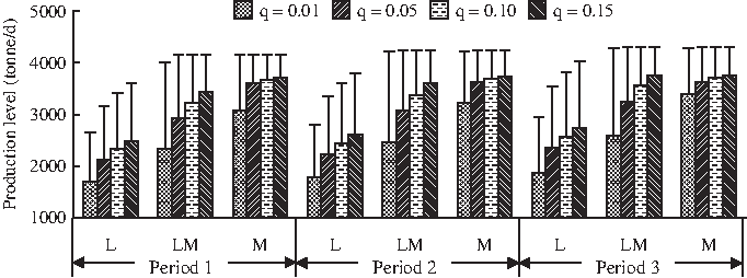
The optimized production levels of the nine dischargers under different water flows and q levels were obtained (as shown in Tables 5 –7). Figure 2 shows the optimized production level of TI, indicating that the production level of TI would increase with an increased water flow. When water flow is low, no production would be allowed for TI under all q levels; this might result from limited BOD load capacity of the river due to the low water flow. When water flows are medium-high and high, the production levels of TI would reach the highest values (no shortage) under any q level; the constraints of water quality requirement would become insignificant under high flow. The results also indicate that the production level of TI would increase with q level since an increased q level brings a relaxed water quality standard and thus a raised pollutant-discharge allowance. The optimized production level for YPP is presented in Fig. 3. The optimized production level for YPP would not be zero even though water flow is low, different from the results for TI. This is because that YPP brings higher benefit when per unit of product to be produced.

FIG. 2.

Optimized production level of TI under different flows and q levels.

FIG. 3.

Optimized production level of YPP under different water flows and q levels.

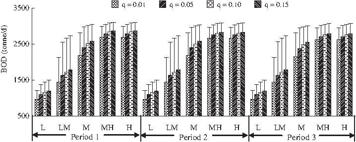
Different water quality requirements (q levels) would result in different production levels of the dischargers, and thus generate different pollution loadings in the river system (as presented in Fig. 4). For example, when the water flow is medium (period 2), under q=0.01, 0.05, 0.10, and 0.15, total amounts of BOD discharges would be [2177, 2962], [2396, 3033], [2502, 3067], and [2576, 3087] ton/day, respectively. In addition, with the increase of water flow, more BOD discharge would be allowed because of higher allowable pollutant capacity in the river system. For instance, when the water flows are low, low-medium, medium, medium-high, and high, the total amounts of BOD discharges (q=0.01) would be [961, 1349], [1440, 2478], [2177, 2962], [2655, 2962], and [2655, 2962] ton/day, respectively.

FIG. 4.

Total amount of BOD discharges under different flows and q levels.

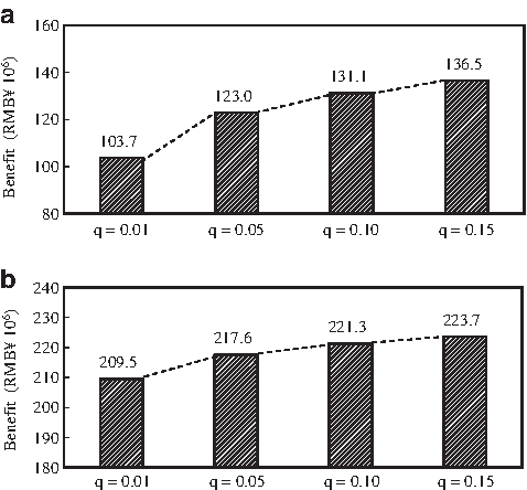
Since the q level represents a set of probabilities at which the constraints would be violated, the relationship between f^± and q demonstrates a tradeoff between system benefit and constraint-violation risk. An increased q means a raised risk of constraint violation and, at the same time, it will lead to a decreased strictness for the water quality constraints. Such a decreased strictness, however, would be linked to a potentially deteriorated water quality. Figure 5 presents the system benefits under the different q levels. Decisions at a lower q level would lead to an increased reliability in fulfilling the water quality requirements but with a lower system benefit; in comparison, decisions at a higher q level would result in a higher system benefit, but the risk of violating the constraints would be increased.

FIG. 5.

Relationship between system benefits and q levels: (a) lower and (b) upper bounds.

Conclusions

In this study, a TIPP method has been developed for river water quality management. The TIPP integrates TSP and ICCP by allowing uncertainties presented as both probability distributions and discrete intervals. It can be used for analyzing various policy scenarios that are associated with different levels of economic penalties when the promised policy targets are violated. Moreover, it can also help examine the tradeoff between the system benefit and the constraint-violation risk under uncertainty. The developed TIPP has been applied to planning water quality management in the Zhangweinan River Basin, China. A number of environmental and economic factors have been integrated into the modeling framework and dynamic interactions between pollutant loading (i.e., production level) and water quality can be reflected. The results for optimized production levels of nine point dischargers under different conditions have been generated. Under the same water flow, the production level of the dischargers would increase with the increase of q level, because an increased q level means relaxed water quality standards and thus raised pollutant-discharge allowances. The results obtained could help support (a) adjustment or justification of production patterns of regional industry; (b) formulation of local policies regarding river water quality protection, economic development, and industry structure; and (c) analysis of interactions among economic benefit, water quality requirement, and environmental penalty. Besides, in practical applications, the solutions from the proposed model are suitable for a preliminary evaluation of various alternatives and for identifying the important data requirement before initiation of more extensive or expensive data collection and simulation studies. The model solution would be more applicable, if postmodeling analyses such as multicriteria decision analysis, group decision making, and public survey can be performed.

Although reasonable solutions have been obtained from the TIPP model, some research extensions have to be done. In this study, relatively simple techniques (i.e., Streeter–Phelps model and the one-dimensional mixing model) were used to simulate water quality, with BOD and DO levels being the main water quality indicators. However, the S-P model was limited by the assumptions of steady state flow in each river segment, without any dispersive effects being considered. If the river system has large fluctuations in its flow rate or there exists significant dispersive effects across different river segments, the model might not be appropriate and would bring considerable errors into the optimization model solutions. Moreover, BOD and DO are considered as the main water quality indicators; this situation is suitable to point-source pollution controls for water bodies in the vicinity of urban zones. In many practical problems, more water quality indicators, such as nitrogen and phosphates, need to be incorporated to tackle non–point source pollution from agricultural sectors. Therefore, more complicated water quality simulation models with multiconstituents need to be advanced for dealing with such complexities. In addition, the water allocation to three diversion canals was simplified in this study. In fact, the water allocation scheme might change with different water quality management schemes. Consequently, the integration of water quantity and water quality management in the study system deserves future research efforts.

Footnotes

Acknowledgments

This research was supported by the Natural Sciences Foundation of China (51190095), Changjiang Scholars and Innovative Research Team in University (IRT1127), and the Program for New Century Excellent Talents in University (NCET-10-0376). The authors are grateful to senior engineer Yu, W.D., and engineer Tian, S.C., in Administration of Zhangweinan River for their provisions of useful data. The authors are grateful to the editor and the anonymous reviewers for their insightful comments and suggestions.

Author Disclosure Statement

No competing financial interests exist.

*

Design and Research Institute of Zhangweinan River Administration (DRIZRA). (Unpublished technical report, 2008). Management Policy and Operation Regulation Report of Yuecheng Reservoir.

†

Editorial Board of Chorography of Zhangweinan River (EBCZR). (Unpublished technical report, 2003). Chorography of Zhangweinan River.

‡

Global Environment Facility (GEF). (Unpublished technical report, 2007). Integrated Water Management Strategic Plan of Zhangweinan River Basin: Base-line Investigation Report.

*

DRIZRA, unpublished (2008).

‡

GEF, unpublished (2007).

References

Birge

J.R.

, Louveaux

F.V.

1997. Introduction to Stochastic Programming. New York: Springer.

Burn

D.H.

, McBean

E.A.

1987. Application of nonlinear optimization to water quality. Appl. Math. Model., 11:438.

Chan

1994. Partial infeasibility method for chance-constrained aquifer management. J. Water Resour. Plann. Manage. (ASCE), 120:70.

Charnes

, Cooper

W.W.

, Kirby

1972. Chance constrained programming: An extension of statistical method. Rustagi

J.S.

Optimizing Methods in Statistics. New York: Academic, 391.

Eckenfelder

W.W.

Jr.

2000. Industrial Water Pollution Control, 3rd. New York: McGraw-Hill.

Huang

G.H.

1996. IPWM: An interval parameter water quality management model. Eng. Optimiz., 26:79.

Huang

G.H.

1998. A hybrid inexact-stochastic water management model. Eur. J. Oper. Res., 107:137.

Huang

G.H.

, Loucks

D.P.

2000. An inexact two-stage stochastic programming model for water resources management under uncertainty. Civ. Eng. Environ. Syst., 17:95.

Huang

W.C.

, Liaw

S.L.

, Chang

S.Y.

2010. Development of a systematic object-event data model of the database system for industrial wastewater treatment plant management. J. Environ. Inform., 15:14.

10.

Karmakar

, Mujumdar

P.P.

2006. An inexact optimization approach for river water-quality management. J. Environ. Manage., 81:233.

11.

, Li

Y.P.

, Li

C.H.

, Huang

G.H.

2010. An inexact two-stage water management model for planning agricultural irrigation under uncertainty. Agric. Water Manage., 97:1905.

12.

Y.P.

, Huang

G.H.

2007. An inexact multistage stochastic quadratic programming method for planning water resources systems under uncertainty. Environ. Eng. Sci., 24:1377.

13.

Y.P.

, Huang

G.H.

2009. Two-stage planning for sustainable water-quality management under uncertainty. J. Environ. Manage., 90:2402.

14.

Y.P.

, Huang

G.H.

, Nie

S.L.

, Qin

X.S.

2007. ITCLP: An inexact two-stage chance-constrained program for planning waste management systems. Resour. Conserv. Recycl., 49:284.

15.

Y.P.

, Huang

G.H.

, Sun

. 2011. Management of uncertain information for environmental systems using a multistage fuzzy-stochastic programming model with soft constraints. J. Environ. Inform., 18:28.

16.

, Huang

G.H.

, Li

Y.P.

, Yang

Z.F.

, Liu

, Cheng

G.H.

2010. Planning regional water resources system using an interval fuzzy bi-level programming method. J. Environ. Inform., 16:43.

17.

Ongley

E.D.

2000. Water quality management: Design, financing and sustainability considerations—II. Invited presentation at the World Bank's Water Week Conference: Towards a Strategy for Managing Water Quality Management, April 3–4, Washington, DC.

18.

Ping

, Chen

, Howboldt

2010. A robust statistical analysis approach for pollutant loadings in urban rivers. J. Environ. Inform., 16:35.

19.

Qin

X.S.

, Huang

G.H.

2009. An inexact chance-constrained quadratic programming model for stream water quality management. Water Resour. Manage., 23:661.

20.

Ruszczynski

, Swietanowski

1997. Accelerating the regularized decomposition method for two-stage stochastic linear problems. Eur. J. Oper. Res., 101:328.

21.

Streeter

H.W.

, Phelps

E.B.

1925. US Public Health Service. Bulletin No. 146: New York.

22.

Thomann

R.V.

, Mueller

J.A.

1987. Principles of Surface Water Quality Modeling and Control. New York: Harper & Row Inc.

23.

U.S. Environmental Protection Agency (USEPA). 1981. Quality Criteria for Water. Washington, D.C.: USEPA.

24.

Xie

Y.L.

, Li

Y.P.

, Huang

G.H.

, Li

Y.F.

2011. An inexact chance-constrained programming model for water quality management in Binhai New Area of Tianjin, China. Sci. Total Environ., 409:1757.

25.

Zhao

, Xia

X.H.

, Yang

Z.F.

, Xia

2011. Temporal and spatial variations of nutrients in Baiyangdian Lake, North China. J. Environ. Inform., 17:102.