Speed Profiles for Improvement of Maritime Emission Estimation

Abstract

Maritime emissions play an important role in anthropogenic emissions, particularly for cities with busy ports such as Hong Kong. Ship emissions are strongly dependent on vessel speed, and thus accurate vessel speed is essential for maritime emission studies. In this study, we determined minute-by-minute high-resolution speed profiles of container ships on four major routes in Hong Kong waters using Automatic Identification System (AIS). The activity-based ship emissions of NO_x, CO, HC, CO₂, SO₂, and PM₁₀ were estimated using derived vessel speed profiles, and results were compared with those using the speed limits of control zones. Estimation using speed limits resulted in up to twofold overestimation of ship emissions. Compared with emissions estimated using the speed limits of control zones, emissions estimated using vessel speed profiles could provide results with up to 88% higher accuracy. Uncertainty analysis and sensitivity analysis of the model demonstrated the significance of improvement of vessel speed resolution. From spatial analysis, it is revealed that SO₂ and PM₁₀ emissions during maneuvering within 1 nautical mile from port were the highest. They contributed 7%–22% of SO₂ emissions and 8%–17% of PM₁₀ emissions of the entire voyage in Hong Kong.

Introduction

Despite increased attention to vehicular air pollution, many scholars have shown that ships are a highly polluting mode of transportation, and they contribute significant sulfur and nitrogen emissions (Corbett and Fischbeck, 1997; Corbett and Koehler, 2003; Endresen et al., 2003; Wang et al., 2007). Exhaust from ships is a major source of sulfur emissions, with a growing contribution from Asia (Streets et al., 2000).

Regardless of the effect of fuel consumption and ship operation costs, vessel speed influences ship emissions. Ship emission is closely associated with engine load, which generally varies by the cube of speed according to the Propeller Law; hence, emissions of pollutants are strongly speed-dependent (PSMAF, 2007). Vessel speed varies in different operational modes, including (i) cruising (at sea), (ii) slow cruising (in reduced speed zone), (iii) maneuvering (to berth), and (iv) hotelling (at berth) (Corbett and Koehler, 2003). With respect to vessel speed, some inventory studies applied an average speed value (or engine load factor) for each operational mode or made an assumption of the same value as the speed limit in the harbor (CARB, 2005; Winther, 2008; Tzannatos, 2010). Although the assumption is reasonable for the regional-scale emission inventory, it may not be detailed enough for the local scale.

Hong Kong has one of the busiest ports in the world, and busy traffic in the sea contributes considerably to ship emissions in Hong Kong waters. Although motor vehicular emissions are a major source of air pollution in urban areas (Harley et al., 2005; Hamdi et al., 2008), it has been suggested that ship emissions are one of the significant sources of particulate matter in Hong Kong and even in the Pearl River Delta region (Cheng et al., 2006; Lee et al., 2006). The estimation of ship emissions is an indispensable task for regional governments and researchers. However, vessel speed information for maritime emission estimation is limited. Container ships are the major emission sources among international shipping. They accounted for 63% of arrival of ocean-going vessels (OGVs) in Hong Kong in 2008 (Marine Department, 2008). In this study, the vessel speed profiles of container ships in Hong Kong waters have been determined using information from Automatic Identification System (AIS) stipulated by the International Maritime Organization (IMO). Ship emissions for different pollutants (i.e., NO_x, CO, HC, CO₂, SO₂, and PM₁₀) were estimated using the vessel speed profile. Results were compared with the method using the speed limits of control zones.

Methodology

Scope

The geographical domain of the current study was the boundary of the Hong Kong Special Administrative Region (HKSAR). The Kwai Chung and Tsing Yi Container Terminals (114°7′ E, 22°20′ N) is the main container port facility in Hong Kong. East Lamma Channel (ELC) and Urmston Road (UR) are two major fairways toward the terminals. Figure 1 shows the geographic domain and the locations of terminals and the major fairways. In this study, only vessels in transiting mode were considered, but not those in hotelling mode.

FIG. 1.

Routes of East Lamma Channel (ELC) and Urmston Road (UR) toward Kwai Chung and Tsing Yi Terminals.

Speed profile

The activities and vessel speeds of a total of 127 container ships on two major fairways were observed from May to September 2009 using the Ship Track System, originated from AIS, provided by the Marine Department. AIS, a traffic information system based on very high-frequency radio transmission, is used globally to track ships for safety and security purposes. Uncertainty associated with human error and detectable error was reported (Harati-Mokhtari et al., 2007); however, AIS is generally an aid providing useful and fast-updated information to the user. By using the Ship Track System, real-time actual speeds of container ships were recorded at high resolution on a 1-min interval, and the speed profile of the entire voyage was obtained for each ship. The vessel speeds of ships on the same route (i.e., ELC arrival, ELC departure, UR arrival, and UR departure) were grouped together and averaged by minute. A general vessel speed profile along the time was generated for each major route.

Emission estimation approach

The emission calculation method employed in this study is an activity-based approach using the following generic equation (USEPA, 2006): \documentclass{aastex}\usepackage{amsbsy}\usepackage{amsfonts}\usepackage{amssymb}\usepackage{bm}\usepackage{mathrsfs}\usepackage{pifont}\usepackage{stmaryrd}\usepackage{textcomp}\usepackage{portland, xspace}\usepackage{amsmath, amsxtra}\pagestyle{empty}\DeclareMathSizes{10}{9}{7}{6}\begin{document} \begin{align*}E = P \times LF \times A \times EF \tag{1}\end{align*} \end{document}

where E is engine emission (g), P is engine power (kW), LF is the engine load factor, A is ship activity (h), and EF is the emission factor (g/[kW·h]). The main engine load factor is expressed as the ratio of a power output to the maximum continuous rated power of a ship under a given speed. The engine load factor was estimated by the Propeller Law based on the following equation: \documentclass{aastex}\usepackage{amsbsy}\usepackage{amsfonts}\usepackage{amssymb}\usepackage{bm}\usepackage{mathrsfs}\usepackage{pifont}\usepackage{stmaryrd}\usepackage{textcomp}\usepackage{portland, xspace}\usepackage{amsmath, amsxtra}\pagestyle{empty}\DeclareMathSizes{10}{9}{7}{6}\begin{document} \begin{align*}LF = ( AS / MS ) ^3 \tag{2}\end{align*} \end{document}

where LF is the engine load factor, AS is actual speed (knots), and MS is maximum speed (knots). There is a dead-slow speed setting with an average of 5.8 knots, and hence a lower limit of engine load factor of 2% was generally adopted (Aldrete et al., 2005). For the auxiliary engine, the same activity-based calculation formula was applied. However, because they are used for electricity supply and not in propulsion (Deniz and Kilic, 2010), their loads are independent from the vessel speed. The auxiliary engine load factors were obtained from a technical report (USEPA, 2006). The emission factors for different pollutants were kept constant until below 20% engine load, at which the emission factors could increase as the load decreases (Jalkanen et al., 2009). Then, emission factor adjustments were adopted for this correction. The ship emissions at every minute for each trip was determined based on Equation (1), and the total emissions from each trip was calculated by summation.

Data input

The schematic diagram of the emission estimation in this study is illustrated in Figure 2. The container ships on the two fairways were identified and tracked. The average vessel speed profile was obtained as described above and applied to the actual speed (AS) in Equation (2). Ship attributes, such as cruise speed, main engine power, engine speed, and the year the targeted ships were built, were collected from World Shipping Encyclopedia. The maximum speed (MS) was determined by dividing the cruise speed by 0.94 (Lloyd's, 2008). The auxiliary engine power was derived by the typical container auxiliary-to-propulsion engine power ratio of 0.22. Emission factors integrated from four comprehensive maritime studies (Lloyd's, 1995; Entec, 2002; Aldrete et al., 2005; USEPA, 2006) were applied as shown in Table 1. The emission factors of SO₂ are fuel quality (sulfur content) dependent. The sulfur contents of 2.37% (mass%) and 1.5% were assumed for main engine fuel and auxiliary engine fuel, respectively, based on the 2008 worldwide average figure from the IMO annual study and on the assumption in Entec's study (Entec, 2002; IMO, 2008). The adjustment factors developed by Aldrete and colleagues are shown in Table 2.

FIG. 2.

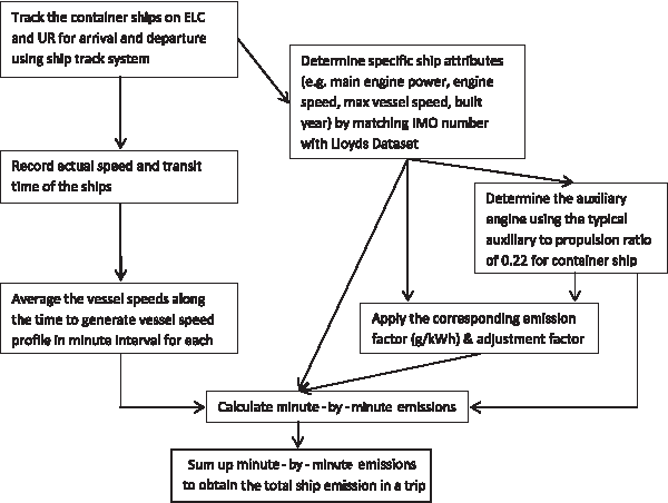
Systematic diagram of emission calculation using vessel speed profiles.

Table 1.

Emission Factors for Main Engines and Auxiliary Engines

	Emission (g/[kW·h])
Engine type and era of manufacture	NO_x ^a	CO ^b	HC ^a	CO₂ ^a	SO₂ ^c	PM₁₀ ^d
Main engines
SSD, pre-2000	18.1	1.4	0.6	620	4.2×%S	1.05
SSD, post-2000	17	1.4	0.6	620	4.2×%S	1.05
MSD, pre-2000	14	1.1	0.5	677	4.2×%S	1.11
MSD, post-2000	13	1.1	0.5	677	4.2×%S	1.11
HSD	12.7	1.1	0.2	677	4.2×%S	1.11
Auxiliary engines
MSD	13.9	1.1	0.4	690	4.2×%S	0.71

Sources: ^aEntec (2002); ^bAldrete et al. (2005); ^cLloyd's (1995); ^dUSEPA (2006).

SSD, slow-speed diesel; MSD, medium-speed diesel; HSD, high-speed diesel.

Table 2.

Emission Factor Adjustment Factors at Low Loads

Load	NO_x	CO	HC	CO₂	SO₂	PM₁₀
1	11.47	20.00	89.44	1.10	1.00	19.17
2	4.63	10.00	31.62	1.10	1.00	7.29
3	2.92	6.67	17.21	1.10	1.00	4.33
4	2.21	5.00	11.18	1.10	1.00	3.09
5	1.83	4.00	8.00	1.10	1.00	2.44
6	1.60	3.33	6.09	1.10	1.00	2.04
7	1.45	2.86	4.83	1.10	1.00	1.79
8	1.35	2.50	3.95	1.10	1.00	1.61
9	1.27	2.22	3.31	1.10	1.00	1.48
10	1.22	2.00	2.83	1.10	1.00	1.38
11	1.17	1.82	2.45	1.10	1.00	1.30
12	1.14	1.67	2.15	1.10	1.00	1.24
13	1.11	1.54	1.91	1.10	1.00	1.19
14	1.08	1.43	1.71	1.10	1.00	1.15
15	1.06	1.33	1.54	1.10	1.00	1.11
16	1.05	1.25	1.40	1.10	1.00	1.08
17	1.03	1.18	1.28	1.10	1.00	1.06
18	1.02	1.11	1.17	1.10	1.00	1.04
19	1.01	1.05	1.08	1.10	1.00	1.02
20	1.00	1.00	1.00	1.00	1.00	1.00

Evaluation of the estimation method using the speed profiles

Emission estimation using vessel speed profiles was evaluated by comparing the emission estimation with the parameter of actual speed substituted by (i) the individual speed data to evaluate the reliability of the method and by (ii) speed limits of the control zones. Data on the individual speed obtained from the AIS were specific to the corresponding trips of the ships, and they were assumed as the real speed data. For the speed limits of the control zone, the data were acquired from the Shipping and Port Control Regulations (BLIS, 2000). A speed limit of 15 knots for slow cruising inside the harbor and a speed limit of 10 knots for maneuvering were adopted. Ship-specific cruise speed from Lloyd's data was employed for ships outside the speed-control zone.

Results and Discussion

Vessel speed profiles

The time average general speed profile for each route is plotted in Figure 3a–d. From the vessel speed profile, the speed variations in different activities along the time were obtained. The drop in each curve was caused by the reduction to a safe speed for piloting (boarding or unboarding of pilots). The patterns of the vessel speed on the two fairways are similar for both arrival and departure, but the speeds and duration on the two fairways are different. The speed profile for each route was divided into slow cruising and maneuvering modes. The results in Table 3 show that in the four routes, the average slow cruising and maneuvering speeds ranged from 9.4 knots to 11.9 knots and from 2.6 knots to 5.2 knots, respectively. The ships were at higher maneuvering speed with shorter duration when departing from berths than when arriving to berths. The three-step speed profile from the control zone method was generated and compared. Figure 4 demonstrates that the vessel speed derived using the control zone method was much higher than that using the vessel speed profile from AIS. The distinct speed variation along the time shows that two- or three-staged speed values are not adequate to represent the speed for the whole trip.

FIG. 3.

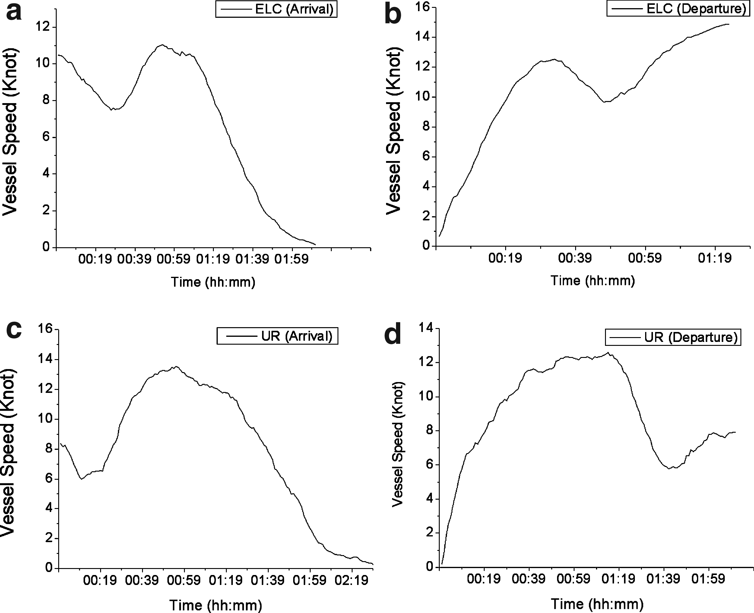
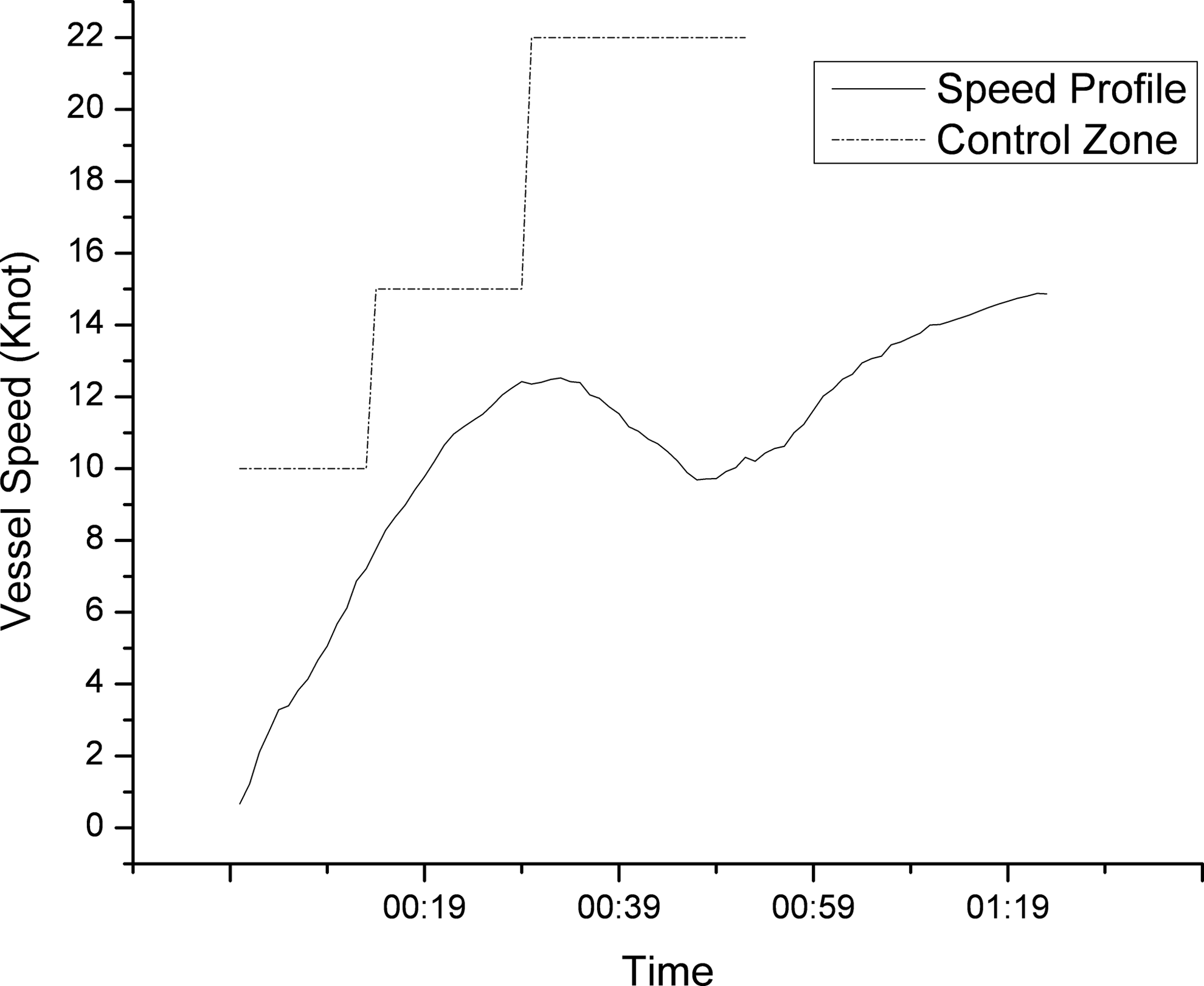
Vessel speed profiles for (a) ship arrival on ELC, (b) ship departure on ELC, (c) ship arrival on UR, and (d) ship departure on UR.

FIG. 4.

Vessel speed plot for vessel speed profile and speed limit of control zone for ship departure on ELC.

Table 3.

Vessel Speed and Transit Duration in Different Operational Modes

	ELC arrival		ELC departure		UR arrival		UR departure
Mode	Speed (knots)	Duration (h:min)	Speed (knots)	Duration (h:min)	Speed (knots)	Duration (h:min)	Speed (knots)	Duration (h:min)
Slow cruising	9.4	01:19	11.9	01:08	10.4	01:38	9.6	01:51
Maneuvering	2.8	00:51	4.3	00:14	2.6	00:54	5.2	00:19

ELC, East Lamma Channel; UR, Urmston Road.

Emission estimation and evaluation

The route-specific vessel speed profiles for the ships on the four routes were applied as the actual speed to calculate the ship emissions for different pollutants, and the results are shown in Table 4. The emission rates from ships on the ELC and UR were similar during arrival. However, the emission rates from ships on the ELC were higher than those on UR because of the higher vessel speed for departure.

Table 4.

Summary of Ship Emission Rate Estimation for Each Route (kg/[N·M])

	NO_x	CO	HC	CO₂	SO₂	PM₁₀
ELC arrival
Average	9.08	1.08	0.73	334.49	3.67	0.58
Minimum	2.76	0.27	0.13	106.72	1.28	0.16
Maximum	21.73	2.72	2.00	781.50	8.27	1.44
Standard deviation	5.40	0.70	0.54	188.69	1.93	0.36
ELC departure
Average	9.99	1.11	0.67	371.08	4.63	0.64
Minimum	3.99	0.33	0.15	146.52	2.08	0.23
Maximum	17.41	2.06	1.30	645.17	7.80	1.14
Standard deviation	4.39	0.58	0.39	160.36	1.84	0.30
UR arrival
Average	12.09	1.36	1.36	455.95	5.15	0.77
Minimum	3.07	0.29	0.29	119.33	1.54	0.19
Maximum	21.24	2.45	2.45	797.99	8.93	1.38
Standard deviation	5.05	0.62	0.62	188.41	2.02	0.34
UR-departure
Average	7.99	0.93	0.65	289.25	3.38	0.53
Minimum	2.95	0.31	0.19	131.96	1.65	0.22
Maximum	19.38	2.45	1.85	671.99	7.48	1.32
Standard deviation	4.70	0.61	0.48	158.62	1.73	0.32

The emission estimates using general vessel speed profiles (E-profile) in this study were evaluated by comparing the estimates using the individual speed data (E-individual) and the estimates using the speed limits of the control zone (E-control zone). The estimation based on individual speed data (E-individual) was regarded as the standard. Correlation analysis was conducted, and the results are shown in Figure 5a–f. In the results, the E-profile was highly correlated with an E-individual. The slopes of 0.95–1.06, which is near 1, for different pollutants demonstrate that the estimated value of the E-profile is close to the standard. On the other hand, the high slopes imply the overestimation of ship emissions using speed limits for various pollutants despite a rather high correlation between the E-control zone and the E-individual. This finding shows that the vessel speed profile is more reliable for the activity-based maritime emission estimation. The discrepancy between the E-control zone and E-profile varied among different pollutants. The discrepancy is more obvious for NO_x, CO₂, SO₂, and PM₁₀, but becomes narrower for CO and HC. The difference is caused by the higher emission adjustment factors at low loads for the estimation of CO and HC emissions, which are more dependent upon engine power. As for higher portion of low engine loads for speed profile than that for speed limits, the higher effect of emission adjustment factors on speed profile compensates for the discrepancy caused by the overestimated speed for speed limits.

FIG. 5.

(a–f) Comparison of ship emission estimations for different pollutants.

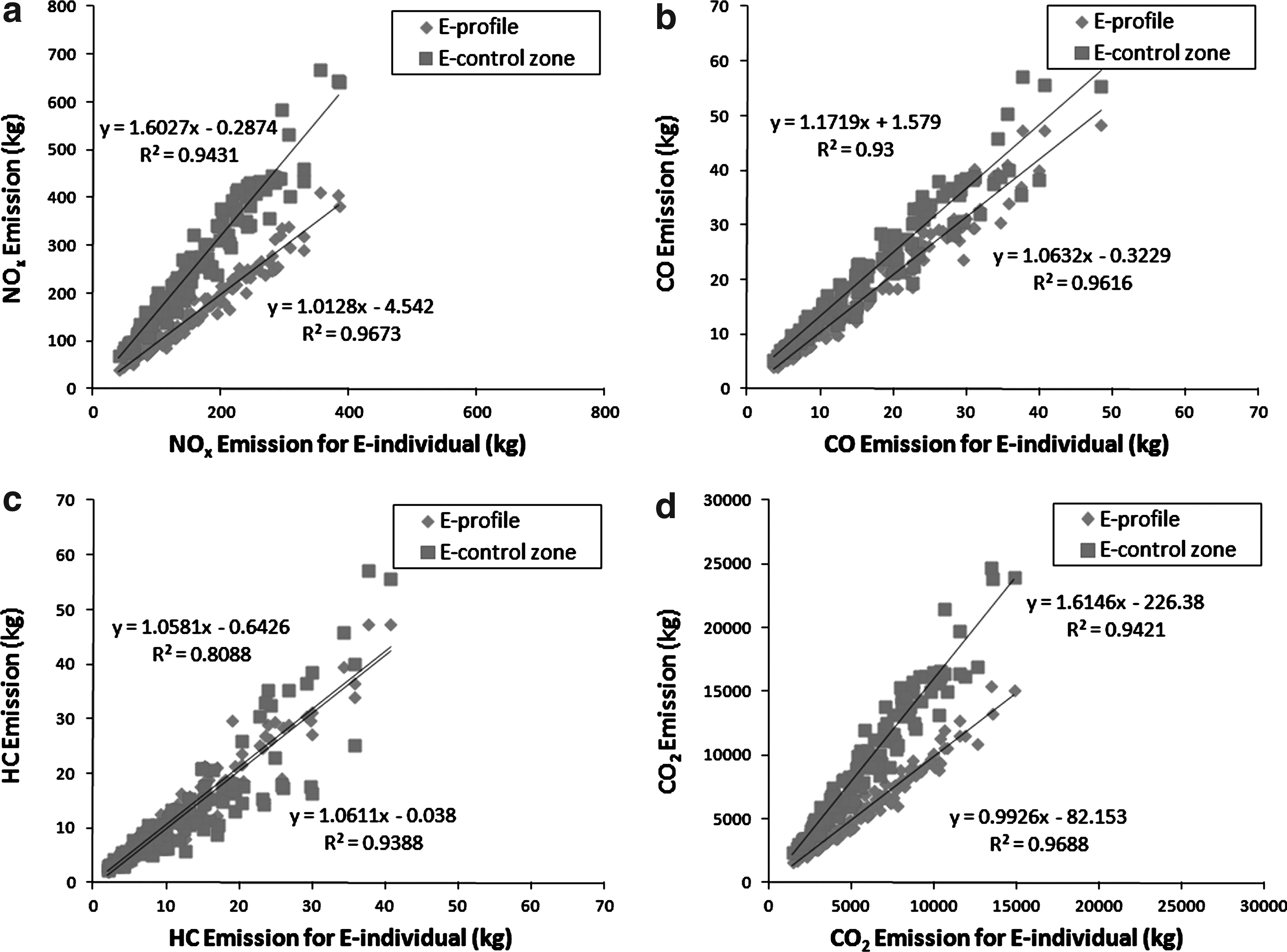
The deviations of the E-profile and E-control zone from the E-individual were evaluated and compared. Table 5 shows that the deviation percentage of emissions with an E-profile from an E-individual is from 6.4%±5.1% (CO₂) up to 13.9%±11.2% (HC). These values are less than those of the speed limits of the E-control zone in the range of 20.5%±14.0% (HC) to 96.0%±25.8% (CO₂). The ship emission estimation using speed profiles significantly improves accuracy by reducing the deviation compared with using the speed limits. This method provides a simple way to generate reliable vessel speed data for emission estimation and the impact assessment of ship emissions to communities.

Table 5.

Deviation Percentage of Estimation with Vessel Speed Profiles and Speed Limits of the Control Zone from Individual Speed Data

Pollutant	Vessel speed profiles (%)	Speed limits of control zone (%)
NO_x	6.7±5.4	60.2±17.7
CO	8.5±6.5	30.5±15.3
HC	13.9±11.2	20.5±14.0
CO₂	6.4±5.1	56.6±17.5
SO₂	8.4±6.4	96.0±25.8
PM₁₀	6.9±5.8	54.8±17.4

Uncertainty and sensitivity analysis

To evaluate the output variability of emission estimates in this model, uncertainty analysis and sensitivity analysis were performed. The Monte Carlo method was adopted to perform multiple evaluations of a model with randomly selected model inputs (Silva et al., 2011). Among the 127 containers, the ship with a median engine power of 25,963 kW was selected for the simulation. For this simulation, SO₂ and PM₁₀ were used to represent the case of more fuel-dependent emission and more engine-condition–dependent emission. Nine general variables were varied between lower, best estimate, and upper bounds as shown in Table 6. Random inputs were generated using triangular distributions, which is an acceptable assumption for those with unknown probabilistic distribution.

Table 6.

Ranges of Inputs for Uncertainty Analysis

Variable	Lower bound	Base-case estimate	Upper bound
AE-to-ME power ratio	−10%	0.22	+10%
Vessel speed (knots)	−20%	From speed profile	+20%
Activity time (h)	−10%	2.23	+10%
Sulfur content in RO (%)	1.5	2.37	3.5
Sulfur content in MDO (%)	−20%	1.5	+20%
PM emission factor (g/[kW·h])
Main engine	−10%	1.05	+10%
Auxiliary engine	−10%	0.71	+10%
Adjustment factors for EF	−10%	Speed dependent	+10%
AE load factor	−10%	Speed dependent	+10%

AE, auxiliary engine; ME, main engine; RO, residual oil; MDO, marine diesel oil; EF, emission factor.

Figure 6a and b presents results of a sensitivity analysis of uncertain input factors by rank correlation for SO₂ and PM₁₀ estimates. For both SO₂ and PM₁₀ emissions, vessel speed was the factor that the emission estimates were the most sensitive to and this agreed with the finding of a previous study (Corbett and Koehler, 2003). The result implies the importance of focusing on the improvement of vessel speed accuracy in this work. Reducing the uncertainty of this input can produce a more accurate estimate. For SO₂ emissions, sulfur content in residual oil was the second most important uncertain input for the estimation. Refining data by a local survey for marine fuel sulfur content may further improve the emission inventory. For PM₁₀ emissions, the adjustment factor for emission factor was the input varying the output most other than the vessel speed. The negative value is due to its reverse relationship with engine load (i.e., with vessel speed). With these adjustment factors, the uncertainty due to emission variation at low engine loads could be refined.

FIG. 6.

Sensitivity analysis of uncertain input factors for (a) SO₂ estimate and (b) PM₁₀ estimate.

Results of uncertainty analysis of SO₂ and PM₁₀ estimates are shown in Figure 7a and b. The best estimates for SO₂ and PM₁₀ emissions for a single ship in the simulation were 53 and 8.4 kg, respectively. They were close to 50th percentiles of the cumulative distribution functions for both SO₂ and PM₁₀. The estimates based on speed limits were 107 and 11.7 kg for SO₂ and PM₁₀ emissions, nearly double and 1.4× the estimates using vessel speed profiles. This illustrates the predictive potential of the vessel speed profiles approach over the speed limits approach.

FIG. 7.

Uncertainty analysis of (a) SO₂ estimate and (b) PM₁₀ estimate.

Spatial distribution of ship emissions

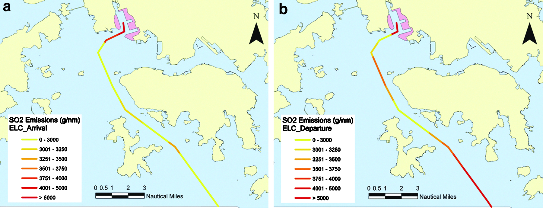
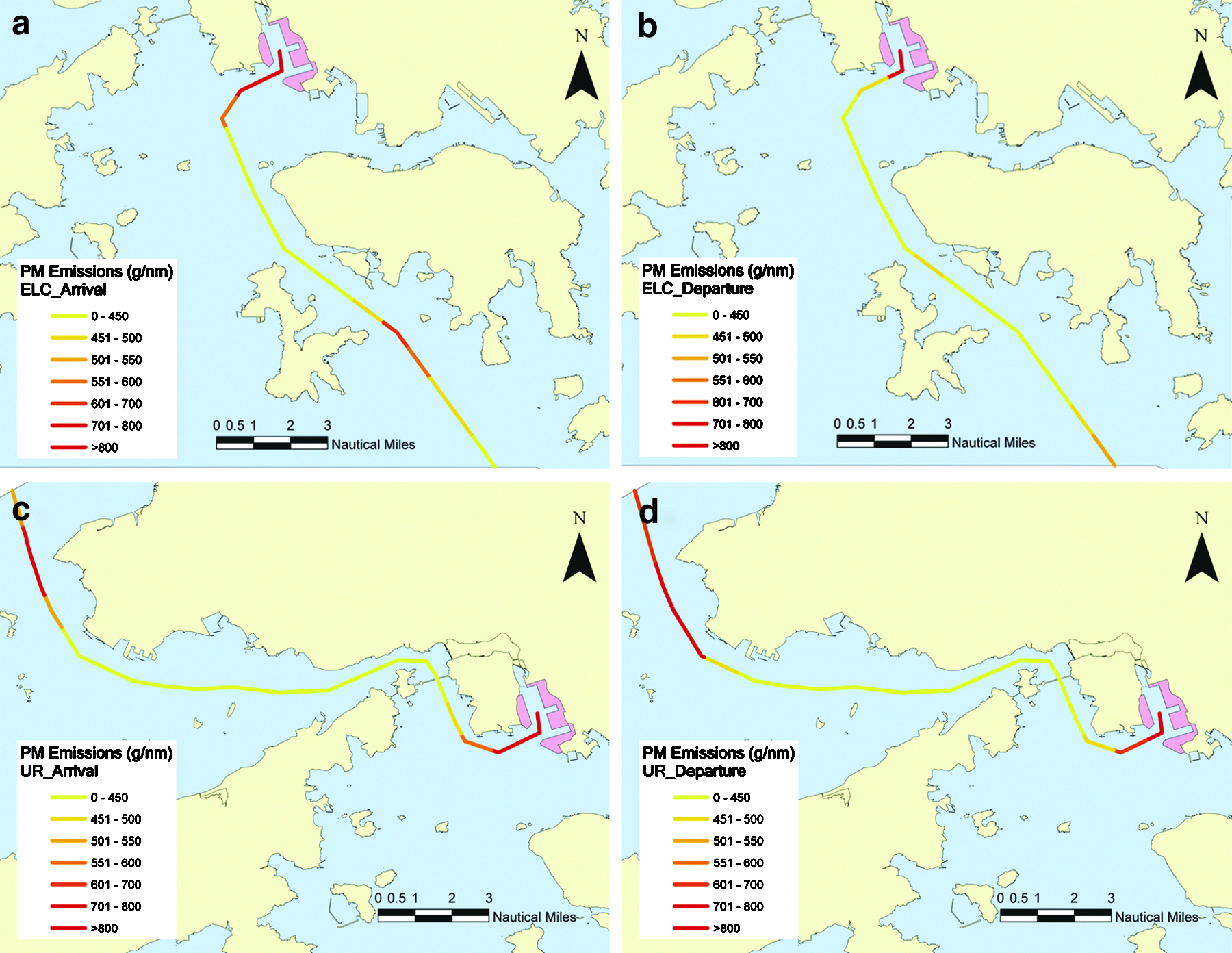
As vessel speed profiles are location (route)-specific, ship emissions can be allocated spatially. The example adopted in the uncertainty analysis was used in this section. The calculated SO₂ and PM₁₀ emissions for a single trip of the container ship were 53, 54, 76, and 68 kg for SO₂, and 8.4, 7.0, 10.0, and 10.7 kg for PM₁₀ on ELC arrival, ELC departure, UR arrival, and UR departure, respectively. The total SO₂ and PM₁₀ emissions for every nautical mile (NM) of the route were calculated, and the emissions per unit NM in each segment were allocated to the four routes with the aid of ArcGIS.

Figures 8 and 9 illustrate the spatial distribution of SO₂ and PM₁₀ emissions from the container ship on different routes. For the ship departure on ELC, the modeled SO₂ emission when leaving Hong Kong waters had a greater amount because of the higher sailing speed when the ship navigates toward open sea. On the other hand, PM₁₀ emissions were high during low engine load (e.g., piloting location). In all four routes, both SO₂ and PM₁₀ emissions near the terminals were highest, because the ship was in a maneuvering mode when the engine load was maintained at around 2%, even if the speed was lower than dead-slow speed. The SO₂ and PM₁₀ emissions from a ship sailing within the segment near the port contributed 22%, 9%, 18%, and 7% SO₂ emissions and 17%, 12%, 15%, and 8% PM₁₀ emissions for ELC arrival, ELC departure, UR arrival, and UR departure, respectively. The emissions for arrival were higher than those for departure, because it takes longer time to berth while approaching. Emissions from ships in the maneuvering mode near the terminals are noticeable, and they may affect the community nearby.

FIG. 8.

(a–d) Spatial distribution of SO₂ emissions from a container ship on different routes.

FIG. 9.

(a–d) Spatial distribution of PM₁₀ emissions from a container ship on different routes.

Conclusions

This study aims to derive vessel speed profiles, which are currently not available, using AIS to provide reliable speed data for maritime emission inventory. Speed variation among the routes demonstrates the role of the route-specific vessel speed profile. Good agreement of emission estimation with the one for individual speed data shows that the general vessel speed profiles derived from AIS provide reliable speed information. Compared with the emissions estimated using speed limits of the control zone, the ship-emission estimation using vessel speed profiles can provide results with up to 88% higher accuracy. The sensitivity analysis and uncertainty analysis demonstrated the importance of the improvement of vessel speed input for emission estimation. This approach also facilitated the spatial distribution of ship emissions. However, it is only limited to the area covered by the AIS base station network, and it may not be applicable to the ships with <300 gross tonnage. Thus, it is more suitable for OGVs. This approach could be further developed to other ship types and minor routes as well as applied to other international ports for the maritime emission investigation.

Footnotes

Acknowledgments

This project was financially supported by a grant from the Research Grants Council of Hong Kong (RGC earmarked grant, PolyU 5210/06E). The authors are grateful to the Marine Department, HKSAR, China, for their valuable information and advice.

Author Disclosure Statement

No competing financial interests exist.

References

Aldrete

, Anderson

, Ray

, Wells

, Durham

, Kristiansson

2005. Port of Los Angeles Baseline Air Emissions Inventory, 2001. Houston, TX: Starcrest Consulting Group, LLC. www.portoflosangeles.org/DOC/REPORT_Final_BAEI_ExecSum.pdf

Department of Justice Bilingual Laws Information System (BLIS). 2000. Shipping and port control regulations—Schedule 4. Speed of VesselsChapter 313AHong Kong: BLIS.

California Environmental Protection Agency—Air Resources Board (CARB). 2005. Emissions Estimation Methodology for Ocean-Going Vessels. Sacramento, CA: CARB.

Cheng

, Lee

S.C.

, Ho

K.F.

, Wang

Y.Q.

, Cao

J.J.

, Chow

J.C.

, Watson

J.G.

2006. Black carbon measurement in a coastal area of south China. J. Geophys. Res., 111:11.

Corbett

J.J.

, Fischbeck

1997. Emissions from ships. Science, 278:823.

Corbett

J.J.

, Koehler

H.W.

2003. Updated emissions from ocean shipping. J. Geophys. Res., 108:15.

Deniz

, Kilic

2010. Estimation and assessment of shipping emissions in the region of Ambarli Port, Turkey. Environ. Prog. Sustain. Energy, 29:107.

Endresen

, Sorgard

, Sundet

J.K.

, Dalsoren

S.B.

, Isaksen

I.S.A.

, Berglen

T.F.

, Gravir

2003. Emission from international sea transportation and environmental impact. J. Geophys. Res.Atmos., 108:4560.

Entec. 2002. Quantification of Emissions from Ships Associated with Ship Movements Between Ports in the European Community (Final Report) Northwich, United Kingdom: Entec UK Ltd.

10.

Hamdi

M.R.

, Bdour

, Tarawneh

2008. Diesel quality in Jordan: Impacts of vehicular and industrial emissions on urban air quality. Environ. Eng. Sci., 25:1333.

11.

Harati-Mokhtari

, Wall

, Brooks

, Wang

2007. Automatic identification system (AIS): Data reliability and human error implications. J. Navig., 60:373.

12.

Harley

R.A.

, Marr

L.C.

, Lehner

J.K.

, Giddings

S.N.

2005. Changes in motor vehicle emissions on diurnal to decadal time scales and effects on atmospheric composition. Environ. Sci. Technol., 39:5356.

13.

International Maritime Organization (IMO). 2008. Prevention of Air Pollution from Ships—Sulphur Monitoring for 2008. Hong Kong: IMO.

14.

Jalkanen

J.P.

, Brink

, Kalli

, Pettersson

, Kukkonen

, Stipa

2009. A modelling system for the exhaust emissions of marine traffic and its application in the Baltic Sea area. Atmos. Chem. Phys., 9:9209.

15.

Lee

S.C.

, Cheng

, Ho

K.F.

, Cao

J.J.

, Louie

P.K.K.

, Chow

J.C.

, Watson

J.G.

2006. PM1.0 and PM2.5 characteristics in the roadside environment of Hong Kong. Aerosol Sci. Technol., 40:157.

16.

Lloyd's. 1995. Marine Exhaust Emissions Research Programme. London: Lloyd's Register.

17.

Lloyd's. 2008. World Shipping Encyclopaedia. London: Lloyd's Register.

18.

Marine Department. 2008. Port of Hong Kong Statistical Tables. Hong Kong: Marine Department.

19.

Puget Sound Maritime Air Forum (PSMAF). 2007. Puget Sound Maritime Air Forum Maritime Air Emissions Inventory. Seattle, WA: PSMAF.

20.

Silva

J.M.N.

, Carreiras

J.M.B.

, Rosa

, Pereira

J.M.C.

2011. Greenhouse gas emissions from shifting cultivation in the tropics, including uncertainty and sensitivity analysis. J. Geophys. Res., 116:21.

21.

Streets

D.G.

, Guttikunda

S.K.

, Carmichael

G.R.

2000. The growing contribution of sulfur emissions from ships in Asian waters, 1988–1995. Atmos. Environ., 34:4425.

22.

Tzannatos

2010. Ship emissions and their externalities for the port of Piraeus—Greece. Atmos. Environ., 44:400.

23.

United States Environmental Protection Agency (USEPA). 2006. Current Methodologies and Best Practices in Preparing Port Emission Inventories. Washington, DC: USEPA.

24.

Wang

C.F.

, Corbett

J.J.

, Winebrake

J.J.

2007. Cost-effectiveness of reducing sulfur emissions from ships. Environ. Sci. Technol., 41:8233.

25.

Winther

2008. New national emission inventory for navigation in Denmark. Atmos. Environ., 42:4632.