Robust Fully Fuzzy Programming with Fuzzy Set Ranking Method for Environmental Systems Planning Under Uncertainty

Introduction

An effective plan for municipal solid waste (MSW) management is one of the major challenges of community decision makers (DMs). Uncertain factors exist in each operating step of MSW systems as a result of various waste generation rates in different times from different producers. Consequently, many optimization methods have been applied to seek an optimization strategy under uncertainty. The majority of the previous optimization methods deal with system uncertainties related to fuzzy linear programming (FLP), stochastic linear programming (SLP), and interval linear programming (ILP) (Huang et al., 1993; He et al., 2009; Jin et al., 2012). The ILP method has proven to be an effective approach because it allows uncertainties to be expressed as interval numbers, which does not lead to complicated intermediate models (Huang et al., 1995). However, the solution created using ILP can cause a violation that contains an infeasible solution under certain conditions. This is also a limitation of dealing with highly uncertain parameters in a model's right and left hand sides (Morgan et al., 1993). The SLP methods are a proper way to deal with probabilistic uncertainties, especially treating a wide range of intervals, as its probabilistic description is known (Zimmermann and Pollatschek, 1975). This feature, however, causes programming defects since the data in the model require knowledge of the parameters' probability distribution. FLP is another method that allows uncertainty to be communicated into the optimization process and results in a deductively rational solution of linguistic ambiguity (Fortemps and Roubens, 1996). However, the main shortcoming of an FLP method is that it is very difficult to observe its membership information.

One desirable approach for dealing with the above issues is through the introduction of the concepts of an interactive method resolution and robust two-step algorithm (RTSM) into an interactive interval FLP framework. This framework will lead to a robust interactive interval fully fuzzy linear programming (RIIFFLP) method. There are four main advantages of this RIIFFLP approach. The first is that the RIIFFLP can allow all model parameters as fuzzy number, including the objective function value. Second, RIIFFLP permits interactive participation of authority in all decision processes. Each interval value in degree α or α-cut (Jiménez, 1996) will be useful for DMs to justify the generated alternatives, which improve the objective function value and satisfy all constraints. Third, the RIIFFLP does not need distribution information for model parameters because it can be easily defined as an interval. Fourth, this new approach not only addresses explicitly a balanced solution between the function objective and the requirement of the constraints, but also ensures no infeasible solution in constraints embedded under the interval solution. It can allow the DMs to have information about the risk of violation of constraints in all the steps of the solution process (Jiménez et al., 2007). Thus, the objective of this research is to propose a new robust interval fully fuzzy programming for MSW management decision making under uncertainty.

Methodology

In environmental systems, for example, MSW management systems, many methods have been developed for dealing with uncertainties in the systems. To date, one of the most effective is the gray linear programming (GLP) (Huang, 1992), as follows: \documentclass{aastex}\usepackage{amsbsy}\usepackage{amsfonts}\usepackage{amssymb}\usepackage{bm}\usepackage{mathrsfs}\usepackage{pifont}\usepackage{stmaryrd}\usepackage{textcomp}\usepackage{portland, xspace}\usepackage{amsmath, amsxtra}\pagestyle{empty}\DeclareMathSizes{10}{9}{7}{6}\begin{document} \begin{align*}{\rm Min} \otimes f = \otimes (C) \otimes (X) \tag{1{\rm a}}\end{align*} \end{document}

Subject to: \documentclass{aastex}\usepackage{amsbsy}\usepackage{amsfonts}\usepackage{amssymb}\usepackage{bm}\usepackage{mathrsfs}\usepackage{pifont}\usepackage{stmaryrd}\usepackage{textcomp}\usepackage{portland, xspace}\usepackage{amsmath, amsxtra}\pagestyle{empty}\DeclareMathSizes{10}{9}{7}{6}\begin{document} \begin{align*}\otimes (A) \otimes (X)\leq \otimes (B) \tag{1{\rm b}}\end{align*} \end{document} \documentclass{aastex}\usepackage{amsbsy}\usepackage{amsfonts}\usepackage{amssymb}\usepackage{bm}\usepackage{mathrsfs}\usepackage{pifont}\usepackage{stmaryrd}\usepackage{textcomp}\usepackage{portland, xspace}\usepackage{amsmath, amsxtra}\pagestyle{empty}\DeclareMathSizes{10}{9}{7}{6}\begin{document} \begin{align*}\otimes (x_j) \geq0 , \otimes (x_j) \in \otimes (X) , \quad j = 1 , 2 , \ldots , n \tag{1{\rm c}}\end{align*} \end{document}

where \documentclass{aastex}\usepackage{amsbsy}\usepackage{amsfonts}\usepackage{amssymb}\usepackage{bm}\usepackage{mathrsfs}\usepackage{pifont}\usepackage{stmaryrd}\usepackage{textcomp}\usepackage{portland, xspace}\usepackage{amsmath, amsxtra}\pagestyle{empty}\DeclareMathSizes{10}{9}{7}{6}\begin{document} $$\otimes (A) \in \otimes (R) ^{m \times n}$$ \end{document} , \documentclass{aastex}\usepackage{amsbsy}\usepackage{amsfonts}\usepackage{amssymb}\usepackage{bm}\usepackage{mathrsfs}\usepackage{pifont}\usepackage{stmaryrd}\usepackage{textcomp}\usepackage{portland, xspace}\usepackage{amsmath, amsxtra}\pagestyle{empty}\DeclareMathSizes{10}{9}{7}{6}\begin{document} $$\otimes (B) \in \otimes (R) ^{m \times l}$$ \end{document} , and \documentclass{aastex}\usepackage{amsbsy}\usepackage{amsfonts}\usepackage{amssymb}\usepackage{bm}\usepackage{mathrsfs}\usepackage{pifont}\usepackage{stmaryrd}\usepackage{textcomp}\usepackage{portland, xspace}\usepackage{amsmath, amsxtra}\pagestyle{empty}\DeclareMathSizes{10}{9}{7}{6}\begin{document} $$\otimes (C) \in \otimes (R) ^{l \times n}$$ \end{document} . The ⨂(R) denotes a set of uncertain numbers. Due to the uncertainty conditions, the optimal solution of Model (1) is \documentclass{aastex}\usepackage{amsbsy}\usepackage{amsfonts}\usepackage{amssymb}\usepackage{bm}\usepackage{mathrsfs}\usepackage{pifont}\usepackage{stmaryrd}\usepackage{textcomp}\usepackage{portland, xspace}\usepackage{amsmath, amsxtra}\pagestyle{empty}\DeclareMathSizes{10}{9}{7}{6}\begin{document} $$\otimes (\,f^*) \in [\underline {\otimes} (\,f^*) , \overline{\otimes} (\,f^*)]]$$ \end{document} , which is achieved by transforming the model into a TSM. Such solutions mean that the minimum system objective is the lower boundary \documentclass{aastex}\usepackage{amsbsy}\usepackage{amsfonts}\usepackage{amssymb}\usepackage{bm}\usepackage{mathrsfs}\usepackage{pifont}\usepackage{stmaryrd}\usepackage{textcomp}\usepackage{portland, xspace}\usepackage{amsmath, amsxtra}\pagestyle{empty}\DeclareMathSizes{10}{9}{7}{6}\begin{document} $$\underline{\otimes} (\,f^*)$$ \end{document} , and the upper boundary value is \documentclass{aastex}\usepackage{amsbsy}\usepackage{amsfonts}\usepackage{amssymb}\usepackage{bm}\usepackage{mathrsfs}\usepackage{pifont}\usepackage{stmaryrd}\usepackage{textcomp}\usepackage{portland, xspace}\usepackage{amsmath, amsxtra}\pagestyle{empty}\DeclareMathSizes{10}{9}{7}{6}\begin{document} $$\overline {\otimes} (\,f^*)$$ \end{document} as the maximum value. The minimum and maximum values correspond to different decision variables. The adjustment of interval variables can correspond to an interval solution of the objective function.

Unfortunately, in such complicated systems, the lower and upper bounds of some interval parameters can rarely be acquired as deterministic values (Tan et al., 2009). Conversely, system parameters can be easily expressed as fuzzy coefficients due to the different experiences of the DMs. For example, during the summer season in some areas, the generation rate of MSW from municipalities can be much higher than at other seasons. In such cases, it can be easier to build interval data of the waste amount rather than crisp data. Moreover, the waste amounts can be estimated by different managers differently, leading to imprecise data with a fuzzy membership function. This can lead to multiple uncertainties. This means that previous studies of GLP/ILP or other similar programming hardly reflect or fully illustrate such multiple uncertainties. Previous researchers indicate that the fuzzy set theory is almost an efficient tool to handle such vague information. Therefore, interval fuzzy set programming has been introduced for dealing with such uncertainties in parameters and objective functions in MSW management. Interval fuzzy sets can be used to tackle multiple uncertainty features, including coefficient values and their membership degrees. The fully fuzzy model can be formulated as follows: \documentclass{aastex}\usepackage{amsbsy}\usepackage{amsfonts}\usepackage{amssymb}\usepackage{bm}\usepackage{mathrsfs}\usepackage{pifont}\usepackage{stmaryrd}\usepackage{textcomp}\usepackage{portland, xspace}\usepackage{amsmath, amsxtra}\pagestyle{empty}\DeclareMathSizes{10}{9}{7}{6}\begin{document} \begin{align*}{\rm Min} \ \widetilde {f}^{\pm} = \sum \nolimits_{j = 1}^n \widetilde{C}^{\pm}_j X^{\pm}_j \tag{2{\rm a}}\end{align*} \end{document}

Subject to: \documentclass{aastex}\usepackage{amsbsy}\usepackage{amsfonts}\usepackage{amssymb}\usepackage{bm}\usepackage{mathrsfs}\usepackage{pifont}\usepackage{stmaryrd}\usepackage{textcomp}\usepackage{portland, xspace}\usepackage{amsmath, amsxtra}\pagestyle{empty}\DeclareMathSizes{10}{9}{7}{6}\begin{document} \begin{align*}\sum \nolimits_{j = 1}^n \widetilde{A}_{ij}^{\pm}X_j^{\pm} \leq \widetilde{B}_i^{\pm} , \quad I = 1 , 2 , \ldots , m \tag{2{\rm b}}\end{align*} \end{document} \documentclass{aastex}\usepackage{amsbsy}\usepackage{amsfonts}\usepackage{amssymb}\usepackage{bm}\usepackage{mathrsfs}\usepackage{pifont}\usepackage{stmaryrd}\usepackage{textcomp}\usepackage{portland, xspace}\usepackage{amsmath, amsxtra}\pagestyle{empty}\DeclareMathSizes{10}{9}{7}{6}\begin{document} \begin{align*}X_j^{\pm} \geq 0 , \quad j = 1 , 2 , \ldots , n \tag{2{\rm c}}\end{align*} \end{document}

where \documentclass{aastex}\usepackage{amsbsy}\usepackage{amsfonts}\usepackage{amssymb}\usepackage{bm}\usepackage{mathrsfs}\usepackage{pifont}\usepackage{stmaryrd}\usepackage{textcomp}\usepackage{portland, xspace}\usepackage{amsmath, amsxtra}\pagestyle{empty}\DeclareMathSizes{10}{9}{7}{6}\begin{document} $$\widetilde{C}^{\pm} \in \{R \} ^{1 \times n}$$ \end{document} , \documentclass{aastex}\usepackage{amsbsy}\usepackage{amsfonts}\usepackage{amssymb}\usepackage{bm}\usepackage{mathrsfs}\usepackage{pifont}\usepackage{stmaryrd}\usepackage{textcomp}\usepackage{portland, xspace}\usepackage{amsmath, amsxtra}\pagestyle{empty}\DeclareMathSizes{10}{9}{7}{6}\begin{document} $$\widetilde{A}^{\pm} \in \{R \} ^{m \times n}$$ \end{document} , \documentclass{aastex}\usepackage{amsbsy}\usepackage{amsfonts}\usepackage{amssymb}\usepackage{bm}\usepackage{mathrsfs}\usepackage{pifont}\usepackage{stmaryrd}\usepackage{textcomp}\usepackage{portland, xspace}\usepackage{amsmath, amsxtra}\pagestyle{empty}\DeclareMathSizes{10}{9}{7}{6}\begin{document} $$\widetilde{B}^{\pm} \in \{R \} ^{m \times 1}$$ \end{document} , and {R} denotes an interval fuzzy set in the objective function and constraints. \documentclass{aastex}\usepackage{amsbsy}\usepackage{amsfonts}\usepackage{amssymb}\usepackage{bm}\usepackage{mathrsfs}\usepackage{pifont}\usepackage{stmaryrd}\usepackage{textcomp}\usepackage{portland, xspace}\usepackage{amsmath, amsxtra}\pagestyle{empty}\DeclareMathSizes{10}{9}{7}{6}\begin{document} $$X_j^{\pm} \in \{R \} ^{n \times 1}$$ \end{document} and {R} denotes an interval variable. The fuzzy set \documentclass{aastex}\usepackage{amsbsy}\usepackage{amsfonts}\usepackage{amssymb}\usepackage{bm}\usepackage{mathrsfs}\usepackage{pifont}\usepackage{stmaryrd}\usepackage{textcomp}\usepackage{portland, xspace}\usepackage{amsmath, amsxtra}\pagestyle{empty}\DeclareMathSizes{10}{9}{7}{6}\begin{document} $$\widetilde {A}$$ \end{document} , as an example, belongs to the universe X={x} with a membership function \documentclass{aastex}\usepackage{amsbsy}\usepackage{amsfonts}\usepackage{amssymb}\usepackage{bm}\usepackage{mathrsfs}\usepackage{pifont}\usepackage{stmaryrd}\usepackage{textcomp}\usepackage{portland, xspace}\usepackage{amsmath, amsxtra}\pagestyle{empty}\DeclareMathSizes{10}{9}{7}{6}\begin{document} $$\mu_{\tilde {A}} (x) \in [0 , 1]$$ \end{document} (Zadeh, 1965). The membership function has a distribution from 0 to 1. When the value of \documentclass{aastex}\usepackage{amsbsy}\usepackage{amsfonts}\usepackage{amssymb}\usepackage{bm}\usepackage{mathrsfs}\usepackage{pifont}\usepackage{stmaryrd}\usepackage{textcomp}\usepackage{portland, xspace}\usepackage{amsmath, amsxtra}\pagestyle{empty}\DeclareMathSizes{10}{9}{7}{6}\begin{document} $$\mu_{\tilde{A}} (x)$$ \end{document} is closer to 1, it indicates that an element x has a higher membership in Universe X. Otherwise, the value of \documentclass{aastex}\usepackage{amsbsy}\usepackage{amsfonts}\usepackage{amssymb}\usepackage{bm}\usepackage{mathrsfs}\usepackage{pifont}\usepackage{stmaryrd}\usepackage{textcomp}\usepackage{portland, xspace}\usepackage{amsmath, amsxtra}\pagestyle{empty}\DeclareMathSizes{10}{9}{7}{6}\begin{document} $$\mu_{\tilde{A}} (x)$$ \end{document} is closer to 0, which means it represents that an element x has a lower membership to Universe X. The membership function can be viewed as the plausibility degree (Zadeh, 1978). It is defined as a possibility distribution expressed as a numerical \documentclass{aastex}\usepackage{amsbsy}\usepackage{amsfonts}\usepackage{amssymb}\usepackage{bm}\usepackage{mathrsfs}\usepackage{pifont}\usepackage{stmaryrd}\usepackage{textcomp}\usepackage{portland, xspace}\usepackage{amsmath, amsxtra}\pagestyle{empty}\DeclareMathSizes{10}{9}{7}{6}\begin{document} $$\mu_{\tilde{A}} (x)$$ \end{document} value. The previous research, using an α cut concept of a fuzzy set {x}, indicates a set of elements that have a degree of plausibility. The α cut has been defined by (Zimmermann, 1995) as \documentclass{aastex}\usepackage{amsbsy}\usepackage{amsfonts}\usepackage{amssymb}\usepackage{bm}\usepackage{mathrsfs}\usepackage{pifont}\usepackage{stmaryrd}\usepackage{textcomp}\usepackage{portland, xspace}\usepackage{amsmath, amsxtra}\pagestyle{empty}\DeclareMathSizes{10}{9}{7}{6}\begin{document} $$\widetilde {A}_{\alpha} = \{x \mid \mu_{\tilde {A}} (x) \geq{\alpha} \} $$ \end{document} . The \documentclass{aastex}\usepackage{amsbsy}\usepackage{amsfonts}\usepackage{amssymb}\usepackage{bm}\usepackage{mathrsfs}\usepackage{pifont}\usepackage{stmaryrd}\usepackage{textcomp}\usepackage{portland, xspace}\usepackage{amsmath, amsxtra}\pagestyle{empty}\DeclareMathSizes{10}{9}{7}{6}\begin{document} $${\widetilde {A}}_{\alpha}$$ \end{document} is upper semicontinuous closed and bounded intervals represented in an interval canonical form (Klir and Pan, 1998) as follows: \documentclass{aastex}\usepackage{amsbsy}\usepackage{amsfonts}\usepackage{amssymb}\usepackage{bm}\usepackage{mathrsfs}\usepackage{pifont}\usepackage{stmaryrd}\usepackage{textcomp}\usepackage{portland, xspace}\usepackage{amsmath, amsxtra}\pagestyle{empty}\DeclareMathSizes{10}{9}{7}{6}\begin{document} \begin{align*}\mu_{\tilde{A}} (x) = \begin{cases} \begin{matrix}0\hfill \forall \ x \in ( - \infty , \alpha_1] ,\hfill \\ f_{\tilde{A}} (x) {\rm increasing \ on} \ [\alpha_1 , \alpha_2] , \\ 1\hfill \forall \ x \in [\alpha_2 , \alpha_3] , \hfill \\ g_{\tilde{A}} (x) {\rm decreasing \ on} \ [\alpha_3 , \alpha_4] , \\ 0\hfill \forall \ x \in [\alpha_4 , + \infty) ,\hfill \end{matrix}\end{cases}\tag{3}\end{align*} \end{document}

where α₁, α₂, α₃, \documentclass{aastex}\usepackage{amsbsy}\usepackage{amsfonts}\usepackage{amssymb}\usepackage{bm}\usepackage{mathrsfs}\usepackage{pifont}\usepackage{stmaryrd}\usepackage{textcomp}\usepackage{portland, xspace}\usepackage{amsmath, amsxtra}\pagestyle{empty}\DeclareMathSizes{10}{9}{7}{6}\begin{document} $$\alpha_4 \in X$$ \end{document} , and α₁≤α₂≤α₃≤α₄. Most of the problems in MSW management are linear functions. Accordingly, it is assumed that f_Ã(x) and g_Ã(x) are both linear functions. Therefore, the fuzzy set μ_Ã(x) has a trapezoidal membership function. If α₁=α₃, on the other hand, the membership function will be triangular. The above statements apply only to single fuzzy set parameters. However, the imprecise characteristics of MSW management lead all parameters of the modeling process to be fuzzy parameters. This entails dealing with the equation's left hand and right hand side parameters under uncertainty plus the uncertainly of the objective function coefficient. Therefore, based on the above considerations, the fuzzy ranking method (Jiménez, 1996) is introduced to the present model to solve the feasibility and optimality problems rising in this fully fuzzy model. First, this process considers the feasibility under multiple constraint uncertainty. If the function degree of \documentclass{aastex}\usepackage{amsbsy}\usepackage{amsfonts}\usepackage{amssymb}\usepackage{bm}\usepackage{mathrsfs}\usepackage{pifont}\usepackage{stmaryrd}\usepackage{textcomp}\usepackage{portland, xspace}\usepackage{amsmath, amsxtra}\pagestyle{empty}\DeclareMathSizes{10}{9}{7}{6}\begin{document} $$\widetilde {A}$$ \end{document} is larger than \documentclass{aastex}\usepackage{amsbsy}\usepackage{amsfonts}\usepackage{amssymb}\usepackage{bm}\usepackage{mathrsfs}\usepackage{pifont}\usepackage{stmaryrd}\usepackage{textcomp}\usepackage{portland, xspace}\usepackage{amsmath, amsxtra}\pagestyle{empty}\DeclareMathSizes{10}{9}{7}{6}\begin{document} $$\widetilde{B}$$ \end{document} , the characteristics of these two fuzzy sets are as follows: \documentclass{aastex}\usepackage{amsbsy}\usepackage{amsfonts}\usepackage{amssymb}\usepackage{bm}\usepackage{mathrsfs}\usepackage{pifont}\usepackage{stmaryrd}\usepackage{textcomp}\usepackage{portland, xspace}\usepackage{amsmath, amsxtra}\pagestyle{empty}\DeclareMathSizes{10}{9}{7}{6}\begin{document} \begin{align*}\mu_M (\widetilde{A} , \widetilde{B}) = \begin{cases}\begin{matrix}0\hfill {\rm if} \ E_2^A - E_1^B < 0 ,\hfill \\ \displaystyle {E_2^A - E_1^B \over E_2^A - E_1^B - (E_1^A - E_2^B )} {\rm if} \ 0 \in [E_1^A - E_2^B , E_2^A - E_1^B] , \\ 1\hfill {\rm if} \ E_1^A - E_2^B < 0 ,\hfill\end{matrix}\end{cases}\tag{4}\end{align*} \end{document}

where \documentclass{aastex}\usepackage{amsbsy}\usepackage{amsfonts}\usepackage{amssymb}\usepackage{bm}\usepackage{mathrsfs}\usepackage{pifont}\usepackage{stmaryrd}\usepackage{textcomp}\usepackage{portland, xspace}\usepackage{amsmath, amsxtra}\pagestyle{empty}\DeclareMathSizes{10}{9}{7}{6}\begin{document} $$[E_1^A , E_2^A]$$ \end{document} and \documentclass{aastex}\usepackage{amsbsy}\usepackage{amsfonts}\usepackage{amssymb}\usepackage{bm}\usepackage{mathrsfs}\usepackage{pifont}\usepackage{stmaryrd}\usepackage{textcomp}\usepackage{portland, xspace}\usepackage{amsmath, amsxtra}\pagestyle{empty}\DeclareMathSizes{10}{9}{7}{6}\begin{document} $$[E_1^B , E_2^B]$$ \end{document} are the expected interval value of \documentclass{aastex}\usepackage{amsbsy}\usepackage{amsfonts}\usepackage{amssymb}\usepackage{bm}\usepackage{mathrsfs}\usepackage{pifont}\usepackage{stmaryrd}\usepackage{textcomp}\usepackage{portland, xspace}\usepackage{amsmath, amsxtra}\pagestyle{empty}\DeclareMathSizes{10}{9}{7}{6}\begin{document} $$\widetilde{A}$$ \end{document} and \documentclass{aastex}\usepackage{amsbsy}\usepackage{amsfonts}\usepackage{amssymb}\usepackage{bm}\usepackage{mathrsfs}\usepackage{pifont}\usepackage{stmaryrd}\usepackage{textcomp}\usepackage{portland, xspace}\usepackage{amsmath, amsxtra}\pagestyle{empty}\DeclareMathSizes{10}{9}{7}{6}\begin{document} $$\widetilde {B}$$ \end{document} . Therefore, when \documentclass{aastex}\usepackage{amsbsy}\usepackage{amsfonts}\usepackage{amssymb}\usepackage{bm}\usepackage{mathrsfs}\usepackage{pifont}\usepackage{stmaryrd}\usepackage{textcomp}\usepackage{portland, xspace}\usepackage{amsmath, amsxtra}\pagestyle{empty}\DeclareMathSizes{10}{9}{7}{6}\begin{document} $$\mu_M (\widetilde{A} , \ \widetilde{B}) \geq \alpha$$ \end{document} , it has the relationship of \documentclass{aastex}\usepackage{amsbsy}\usepackage{amsfonts}\usepackage{amssymb}\usepackage{bm}\usepackage{mathrsfs}\usepackage{pifont}\usepackage{stmaryrd}\usepackage{textcomp}\usepackage{portland, xspace}\usepackage{amsmath, amsxtra}\pagestyle{empty}\DeclareMathSizes{10}{9}{7}{6}\begin{document} $$\widetilde{A} \geq_{\alpha} \widetilde{B}$$ \end{document} . Then, the \documentclass{aastex}\usepackage{amsbsy}\usepackage{amsfonts}\usepackage{amssymb}\usepackage{bm}\usepackage{mathrsfs}\usepackage{pifont}\usepackage{stmaryrd}\usepackage{textcomp}\usepackage{portland, xspace}\usepackage{amsmath, amsxtra}\pagestyle{empty}\DeclareMathSizes{10}{9}{7}{6}\begin{document} $$\mu_M (\widetilde{A} , \ \widetilde{B})$$ \end{document} is an α-feasible decision under the following assumption, \documentclass{aastex}\usepackage{amsbsy}\usepackage{amsfonts}\usepackage{amssymb}\usepackage{bm}\usepackage{mathrsfs}\usepackage{pifont}\usepackage{stmaryrd}\usepackage{textcomp}\usepackage{portland, xspace}\usepackage{amsmath, amsxtra}\pagestyle{empty}\DeclareMathSizes{10}{9}{7}{6}\begin{document} \begin{align*}{\rm Min} \ \{ \mu_M (\widetilde{A}_i x , \widetilde{B}_i) \} = \alpha \tag{5}\end{align*} \end{document}

where x, \documentclass{aastex}\usepackage{amsbsy}\usepackage{amsfonts}\usepackage{amssymb}\usepackage{bm}\usepackage{mathrsfs}\usepackage{pifont}\usepackage{stmaryrd}\usepackage{textcomp}\usepackage{portland, xspace}\usepackage{amsmath, amsxtra}\pagestyle{empty}\DeclareMathSizes{10}{9}{7}{6}\begin{document} $$\widetilde A_i$$ \end{document} are variables and \documentclass{aastex}\usepackage{amsbsy}\usepackage{amsfonts}\usepackage{amssymb}\usepackage{bm}\usepackage{mathrsfs}\usepackage{pifont}\usepackage{stmaryrd}\usepackage{textcomp}\usepackage{portland, xspace}\usepackage{amsmath, amsxtra}\pagestyle{empty}\DeclareMathSizes{10}{9}{7}{6}\begin{document} $$x \in R^n$$ \end{document} , \documentclass{aastex}\usepackage{amsbsy}\usepackage{amsfonts}\usepackage{amssymb}\usepackage{bm}\usepackage{mathrsfs}\usepackage{pifont}\usepackage{stmaryrd}\usepackage{textcomp}\usepackage{portland, xspace}\usepackage{amsmath, amsxtra}\pagestyle{empty}\DeclareMathSizes{10}{9}{7}{6}\begin{document} $$\widetilde {A}_i = (\widetilde {A}_{i1} , \widetilde {A}_{i2} , \ldots , \widetilde{A}_{in})$$ \end{document} . There is, thus, an α-feasible decision vector. However, 1−α can provide a risk of infeasibility. In such a case, Equation (4) can be transformed into the following pattern (Jiménez et al., 2007): \documentclass{aastex}\usepackage{amsbsy}\usepackage{amsfonts}\usepackage{amssymb}\usepackage{bm}\usepackage{mathrsfs}\usepackage{pifont}\usepackage{stmaryrd}\usepackage{textcomp}\usepackage{portland, xspace}\usepackage{amsmath, amsxtra}\pagestyle{empty}\DeclareMathSizes{10}{9}{7}{6}\begin{document} \begin{align*}[(1 - \alpha) E_2^{Ai} + E_1^{Ai}] x \geq \alpha E_2^{Bi} + (1 - \alpha) E_1^{Bi} \tag{6}\end{align*} \end{document}

The feasible decision α vectors are given as ℵ(α). Then, it becomes evident that the relationship is α₁≤α₂⇒ℵ(α₁) ⊃ ℵ(α₂). Therefore, according to Equations (4)–(6), the feasibility among fuzzy constraint parameters can be solved by using α parameter for an intersection fuzzy set \documentclass{aastex}\usepackage{amsbsy}\usepackage{amsfonts}\usepackage{amssymb}\usepackage{bm}\usepackage{mathrsfs}\usepackage{pifont}\usepackage{stmaryrd}\usepackage{textcomp}\usepackage{portland, xspace}\usepackage{amsmath, amsxtra}\pagestyle{empty}\DeclareMathSizes{10}{9}{7}{6}\begin{document} $$\mu_M (\widetilde{A} , \ \widetilde{B})$$ \end{document} . However, the optimality for the objective function and fuzzy coefficients has to be handled in the next step. According to the fuzzy ranking method, let us assume that vector \documentclass{aastex}\usepackage{amsbsy}\usepackage{amsfonts}\usepackage{amssymb}\usepackage{bm}\usepackage{mathrsfs}\usepackage{pifont}\usepackage{stmaryrd}\usepackage{textcomp}\usepackage{portland, xspace}\usepackage{amsmath, amsxtra}\pagestyle{empty}\DeclareMathSizes{10}{9}{7}{6}\begin{document} $$X^0 \in \aleph (\widetilde{A} , \ \widetilde{B})$$ \end{document} is an acceptable optimal solution for a fully fuzzy linear program; then, the fuzzy coefficient objective function has the following formulation (Jiménez et al., 2007); \documentclass{aastex}\usepackage{amsbsy}\usepackage{amsfonts}\usepackage{amssymb}\usepackage{bm}\usepackage{mathrsfs}\usepackage{pifont}\usepackage{stmaryrd}\usepackage{textcomp}\usepackage{portland, xspace}\usepackage{amsmath, amsxtra}\pagestyle{empty}\DeclareMathSizes{10}{9}{7}{6}\begin{document} \begin{align*}\mu_M (\widetilde {C}X , \widetilde{C}X^0) \geq \alpha_0 , \quad \forall X \in \aleph (A , B) \tag{7}\end{align*} \end{document}

where \documentclass{aastex}\usepackage{amsbsy}\usepackage{amsfonts}\usepackage{amssymb}\usepackage{bm}\usepackage{mathrsfs}\usepackage{pifont}\usepackage{stmaryrd}\usepackage{textcomp}\usepackage{portland, xspace}\usepackage{amsmath, amsxtra}\pagestyle{empty}\DeclareMathSizes{10}{9}{7}{6}\begin{document} $$\widetilde{C}$$ \end{document} is a fuzzy vector and the \documentclass{aastex}\usepackage{amsbsy}\usepackage{amsfonts}\usepackage{amssymb}\usepackage{bm}\usepackage{mathrsfs}\usepackage{pifont}\usepackage{stmaryrd}\usepackage{textcomp}\usepackage{portland, xspace}\usepackage{amsmath, amsxtra}\pagestyle{empty}\DeclareMathSizes{10}{9}{7}{6}\begin{document} $$X^0 \in \ \aleph (A , B)$$ \end{document} is an optimal choice at least to a certain degree, α₀ as opposed to the other feasible vectors. Due to the expression of Equation (4), the objective function fuzzy parameter can be written as \documentclass{aastex}\usepackage{amsbsy}\usepackage{amsfonts}\usepackage{amssymb}\usepackage{bm}\usepackage{mathrsfs}\usepackage{pifont}\usepackage{stmaryrd}\usepackage{textcomp}\usepackage{portland, xspace}\usepackage{amsmath, amsxtra}\pagestyle{empty}\DeclareMathSizes{10}{9}{7}{6}\begin{document} \begin{align*} \frac {E_2^{\widetilde{C} X} - E_1^{\widetilde{C} X^0}} {E_2^{\widetilde{C} X} - E_1^{\widetilde{C} X} + E_1^{\widetilde{C} X^0} - E_2^{\widetilde{C} X^0}} \ge \alpha_0 \tag{8} \end{align*} \end{document}

Based on Equations (6) and (8), the vector \documentclass{aastex}\usepackage{amsbsy}\usepackage{amsfonts}\usepackage{amssymb}\usepackage{bm}\usepackage{mathrsfs}\usepackage{pifont}\usepackage{stmaryrd}\usepackage{textcomp}\usepackage{portland, xspace}\usepackage{amsmath, amsxtra}\pagestyle{empty}\DeclareMathSizes{10}{9}{7}{6}\begin{document} $$X^0 (\alpha) \in R^n$$ \end{document} is an acceptable solution if it is an optimal solution to the following FLP (Jiménez et al., 2007). Then, the first model can be transferred into a new pattern as follows: \documentclass{aastex}\usepackage{amsbsy}\usepackage{amsfonts}\usepackage{amssymb}\usepackage{bm}\usepackage{mathrsfs}\usepackage{pifont}\usepackage{stmaryrd}\usepackage{textcomp}\usepackage{portland, xspace}\usepackage{amsmath, amsxtra}\pagestyle{empty}\DeclareMathSizes{10}{9}{7}{6}\begin{document} \begin{align*}{\rm Min} \ EV (\,\widetilde {f}^{\pm}) = \sum \nolimits_{j = 1}^n EV (\widetilde {C}_j^{\pm}) X_j^{\pm} \tag{9{\rm a}}\end{align*} \end{document}

Subject to: \documentclass{aastex}\usepackage{amsbsy}\usepackage{amsfonts}\usepackage{amssymb}\usepackage{bm}\usepackage{mathrsfs}\usepackage{pifont}\usepackage{stmaryrd}\usepackage{textcomp}\usepackage{portland, xspace}\usepackage{amsmath, amsxtra}\pagestyle{empty}\DeclareMathSizes{10}{9}{7}{6}\begin{document} \begin{align*}(1 - a) \sum \nolimits_{j = 1}^n \left[E_1^{A_{ij}^{\pm}} + aE_2^{A_{ij}^{\pm}}\right] X_j^{\pm} \leq a E_1^{b_i^{\pm}} + (1 - a) \, E_2^{b_i^{\pm}} , \quad i = 1 , 2 , \ldots , m \tag{9{\rm b}}\end{align*} \end{document} \documentclass{aastex}\usepackage{amsbsy}\usepackage{amsfonts}\usepackage{amssymb}\usepackage{bm}\usepackage{mathrsfs}\usepackage{pifont}\usepackage{stmaryrd}\usepackage{textcomp}\usepackage{portland, xspace}\usepackage{amsmath, amsxtra}\pagestyle{empty}\DeclareMathSizes{10}{9}{7}{6}\begin{document} \begin{align*}X_j^{\pm} \geq 0 ,\quad j = 1 , 2 , \ldots , n \tag{9{\rm c}}\end{align*} \end{document}

where \documentclass{aastex}\usepackage{amsbsy}\usepackage{amsfonts}\usepackage{amssymb}\usepackage{bm}\usepackage{mathrsfs}\usepackage{pifont}\usepackage{stmaryrd}\usepackage{textcomp}\usepackage{portland, xspace}\usepackage{amsmath, amsxtra}\pagestyle{empty}\DeclareMathSizes{10}{9}{7}{6}\begin{document} $$EV (\widetilde{C}_j) = [EV (\widetilde{C}_1) , EV (\widetilde {C}_2) , \ldots , EV (\widetilde{C}_n)]$$ \end{document} indicates that it is the expected value for the fuzzy vector \documentclass{aastex}\usepackage{amsbsy}\usepackage{amsfonts}\usepackage{amssymb}\usepackage{bm}\usepackage{mathrsfs}\usepackage{pifont}\usepackage{stmaryrd}\usepackage{textcomp}\usepackage{portland, xspace}\usepackage{amsmath, amsxtra}\pagestyle{empty}\DeclareMathSizes{10}{9}{7}{6}\begin{document} $$(\widetilde{C})$$ \end{document} . To solve this model, the TSM is an effective approach (Huang, 1992). The main idea of TSM is that it converts the interval model into two linear submodels to solve the model. It can provide a number of schemes for DMs if the solutions are feasible. However, the solutions of TSM may lead to violations, which are infeasible solutions. There have been many attempts to modify violation problems. Zhou et al. (2008) developed modified ILP (MILP). Cao and Huang (2011) used a three-step method (ThSM) to avoid solution violation. However, these two methods still have some deficits. The solution of the MILP method is too narrow to provide a comprehensively feasible solution, and the ThSM may cause a long, tedious calculation process that may lead to more decision variables. To deal with the shortcoming of TSM, a RTSM has been developed (Fan and Huang, 2011). RTSM first calculated the conservative submodel, which corresponds to f⁺ as follows: \documentclass{aastex}\usepackage{amsbsy}\usepackage{amsfonts}\usepackage{amssymb}\usepackage{bm}\usepackage{mathrsfs}\usepackage{pifont}\usepackage{stmaryrd}\usepackage{textcomp}\usepackage{portland, xspace}\usepackage{amsmath, amsxtra}\pagestyle{empty}\DeclareMathSizes{10}{9}{7}{6}\begin{document} \begin{align*}{\rm Max} \ f^{-} = \sum \limits_{j = 1}^k c_j^{-}x_j^{-} + \sum \limits_{j = k + 1}^n c_j^{-}x_j^ + \tag{10{\rm a}}\end{align*} \end{document}

Subject to: \documentclass{aastex}\usepackage{amsbsy}\usepackage{amsfonts}\usepackage{amssymb}\usepackage{bm}\usepackage{mathrsfs}\usepackage{pifont}\usepackage{stmaryrd}\usepackage{textcomp}\usepackage{portland, xspace}\usepackage{amsmath, amsxtra}\pagestyle{empty}\DeclareMathSizes{10}{9}{7}{6}\begin{document} \begin{align*} \begin{split}\sum\limits_{j = 1}^k \big| a_{ij}^{\pm} \big| ^ + \ Sign (a_{ij}^{\pm}) x_j^{-} + \sum \limits_{j = k + 1}^n \big| a_{ij}^{\pm} \big| ^{-} \ \\ \quad Sign (a_{ij}^{\pm}) x_j^ + \leq \,b_i^{-} , \quad i = 1 , 2 , \ldots m\end{split} \tag{10{\rm b}} \end{align*} \end{document} \documentclass{aastex}\usepackage{amsbsy}\usepackage{amsfonts}\usepackage{amssymb}\usepackage{bm}\usepackage{mathrsfs}\usepackage{pifont}\usepackage{stmaryrd}\usepackage{textcomp}\usepackage{portland, xspace}\usepackage{amsmath, amsxtra}\pagestyle{empty}\DeclareMathSizes{10}{9}{7}{6}\begin{document} \begin{align*}x_j^{-} \geq \,0 ,\quad j = 1 , 2 , \ldots , k \tag{10{\rm c}}\end{align*} \end{document} \documentclass{aastex}\usepackage{amsbsy}\usepackage{amsfonts}\usepackage{amssymb}\usepackage{bm}\usepackage{mathrsfs}\usepackage{pifont}\usepackage{stmaryrd}\usepackage{textcomp}\usepackage{portland, xspace}\usepackage{amsmath, amsxtra}\pagestyle{empty}\DeclareMathSizes{10}{9}{7}{6}\begin{document} \begin{align*}x_j^ + \geq \,0 ,\quad j = k + 1 , k + 2 , \ldots , n \tag{10{\rm d}}\end{align*} \end{document}

where \documentclass{aastex}\usepackage{amsbsy}\usepackage{amsfonts}\usepackage{amssymb}\usepackage{bm}\usepackage{mathrsfs}\usepackage{pifont}\usepackage{stmaryrd}\usepackage{textcomp}\usepackage{portland, xspace}\usepackage{amsmath, amsxtra}\pagestyle{empty}\DeclareMathSizes{10}{9}{7}{6}\begin{document} $$a^{\pm} \in \{R^{\pm} \} ^{m \times n} , \ \,c^{\pm} \in \{R^{\pm} \} ^{1 \times n} , \,\ b^{\pm} \in \{R^{\pm} \} ^{m \times 1} , \,\ x^{\pm} \,\in \{R^{\pm} \} ^{n \times 1}$$ \end{document} , and {R^±} represent a set of interval numbers with lower and upper bounds. Then, the solution \documentclass{aastex}\usepackage{amsbsy}\usepackage{amsfonts}\usepackage{amssymb}\usepackage{bm}\usepackage{mathrsfs}\usepackage{pifont}\usepackage{stmaryrd}\usepackage{textcomp}\usepackage{portland, xspace}\usepackage{amsmath, amsxtra}\pagestyle{empty}\DeclareMathSizes{10}{9}{7}{6}\begin{document} $$x_{jopt}^{-}$$ \end{document} and \documentclass{aastex}\usepackage{amsbsy}\usepackage{amsfonts}\usepackage{amssymb}\usepackage{bm}\usepackage{mathrsfs}\usepackage{pifont}\usepackage{stmaryrd}\usepackage{textcomp}\usepackage{portland, xspace}\usepackage{amsmath, amsxtra}\pagestyle{empty}\DeclareMathSizes{10}{9}{7}{6}\begin{document} $$x_{jopt}^{+}$$ \end{document} of Equation (8) can be obtained. Next, these two solutions are incorporated into the second submodel to obtain f⁻ as follows: (Assume that \documentclass{aastex}\usepackage{amsbsy}\usepackage{amsfonts}\usepackage{amssymb}\usepackage{bm}\usepackage{mathrsfs}\usepackage{pifont}\usepackage{stmaryrd}\usepackage{textcomp}\usepackage{portland, xspace}\usepackage{amsmath, amsxtra}\pagestyle{empty}\DeclareMathSizes{10}{9}{7}{6}\begin{document} $$b_i^{\pm} > 0$$ \end{document} and f ^±>0), \documentclass{aastex}\usepackage{amsbsy}\usepackage{amsfonts}\usepackage{amssymb}\usepackage{bm}\usepackage{mathrsfs}\usepackage{pifont}\usepackage{stmaryrd}\usepackage{textcomp}\usepackage{portland, xspace}\usepackage{amsmath, amsxtra}\pagestyle{empty}\DeclareMathSizes{10}{9}{7}{6}\begin{document} \begin{align*}{\rm Max} \ f^ + = \sum \limits_{j = 1}^k c_j^{+}x_j^{+} + \sum \limits_{j = k + 1}^n c_j^{+}x_j^{-} \tag{11{\rm a}}\end{align*} \end{document}

Subject to: \documentclass{aastex}\usepackage{amsbsy}\usepackage{amsfonts}\usepackage{amssymb}\usepackage{bm}\usepackage{mathrsfs}\usepackage{pifont}\usepackage{stmaryrd}\usepackage{textcomp}\usepackage{portland, xspace}\usepackage{amsmath, amsxtra}\pagestyle{empty}\DeclareMathSizes{10}{9}{7}{6}\begin{document} \begin{align*} \begin{split} \sum \limits_{j = 1}^k \big| a_{ij}^{\pm} \big| ^{-} \ Sign (a_{ij}^{\pm}) x_j^{+} + \sum \limits_{j = k + 1}^n \big| a_{ij}^{\pm} \big| ^{+} \\ \quad Sign (a_{ij}^{\pm}) x_j^{-} \leq \,b_i^{+} ,\quad i = 1 , 2 , \ldots , m\end{split} \tag{11{\rm b}}\end{align*} \end{document} \documentclass{aastex}\usepackage{amsbsy}\usepackage{amsfonts}\usepackage{amssymb}\usepackage{bm}\usepackage{mathrsfs}\usepackage{pifont}\usepackage{stmaryrd}\usepackage{textcomp}\usepackage{portland, xspace}\usepackage{amsmath, amsxtra}\pagestyle{empty}\DeclareMathSizes{10}{9}{7}{6}\begin{document} \begin{align*}\sum \limits_{j = 1}^{l_{i1}}a_{ij}^{-}x_j^{+} + \sum \limits_{j = l_{i1} + 1}^k a_{ij}^{-}x_{jopt}^{-} + \sum \limits_{j = k + 1}^{l_{i2}} a_{ij}^{-}x_j^{-} + \sum \limits_{j = l_{i2} + 1}^n a_{ij}^{-}x_{jopt}^ + \leq b_i^{+} \tag{11{\rm c}}\end{align*} \end{document} \documentclass{aastex}\usepackage{amsbsy}\usepackage{amsfonts}\usepackage{amssymb}\usepackage{bm}\usepackage{mathrsfs}\usepackage{pifont}\usepackage{stmaryrd}\usepackage{textcomp}\usepackage{portland, xspace}\usepackage{amsmath, amsxtra}\pagestyle{empty}\DeclareMathSizes{10}{9}{7}{6}\begin{document} \begin{align*}x_j^{+} \geq x_{jopt}^{-} \quad j = 1 , 2 , \ldots , k \tag{11{\rm d}}\end{align*} \end{document} \documentclass{aastex}\usepackage{amsbsy}\usepackage{amsfonts}\usepackage{amssymb}\usepackage{bm}\usepackage{mathrsfs}\usepackage{pifont}\usepackage{stmaryrd}\usepackage{textcomp}\usepackage{portland, xspace}\usepackage{amsmath, amsxtra}\pagestyle{empty}\DeclareMathSizes{10}{9}{7}{6}\begin{document} \begin{align*}x_j^{-} \leq x_{jopt}^{+} \quad j = k + 1 , \ldots , n \tag{11{\rm e}}\end{align*} \end{document} \documentclass{aastex}\usepackage{amsbsy}\usepackage{amsfonts}\usepackage{amssymb}\usepackage{bm}\usepackage{mathrsfs}\usepackage{pifont}\usepackage{stmaryrd}\usepackage{textcomp}\usepackage{portland, xspace}\usepackage{amsmath, amsxtra}\pagestyle{empty}\DeclareMathSizes{10}{9}{7}{6}\begin{document} \begin{align*}x_j^{+} \geq 0 , \quad j = 1 , 2 , \ldots , k \tag{11{\rm f}}\end{align*} \end{document} \documentclass{aastex}\usepackage{amsbsy}\usepackage{amsfonts}\usepackage{amssymb}\usepackage{bm}\usepackage{mathrsfs}\usepackage{pifont}\usepackage{stmaryrd}\usepackage{textcomp}\usepackage{portland, xspace}\usepackage{amsmath, amsxtra}\pagestyle{empty}\DeclareMathSizes{10}{9}{7}{6}\begin{document} \begin{align*}x_j^{-} \geq 0 , \quad j = k + 1 , k + 2 , \ldots , n \tag{11{\rm g}}\end{align*} \end{document}

where \documentclass{aastex}\usepackage{amsbsy}\usepackage{amsfonts}\usepackage{amssymb}\usepackage{bm}\usepackage{mathrsfs}\usepackage{pifont}\usepackage{stmaryrd}\usepackage{textcomp}\usepackage{portland, xspace}\usepackage{amsmath, amsxtra}\pagestyle{empty}\DeclareMathSizes{10}{9}{7}{6}\begin{document} $$c_j^{\pm} \geq 0 \ (\,j = 1 , 2 , \ldots , k)$$ \end{document} , and \documentclass{aastex}\usepackage{amsbsy}\usepackage{amsfonts}\usepackage{amssymb}\usepackage{bm}\usepackage{mathrsfs}\usepackage{pifont}\usepackage{stmaryrd}\usepackage{textcomp}\usepackage{portland, xspace}\usepackage{amsmath, amsxtra}\pagestyle{empty}\DeclareMathSizes{10}{9}{7}{6}\begin{document} $$c_j^{\pm} \leq 0 \ (\, j = k + 1 , 2 , \ldots , k) \hbox{;} a_{ij}^{\pm} \geq \,0 \ (\,j = 1 , 2 , \ldots , \ l_{ij}\hbox{;}\ \,j = l_{i2} + 1 , \ l_{i2} + 2 , \ldots , n)$$ \end{document} , and \documentclass{aastex}\usepackage{amsbsy}\usepackage{amsfonts}\usepackage{amssymb}\usepackage{bm}\usepackage{mathrsfs}\usepackage{pifont}\usepackage{stmaryrd}\usepackage{textcomp}\usepackage{portland, xspace}\usepackage{amsmath, amsxtra}\pagestyle{empty}\DeclareMathSizes{10}{9}{7}{6}\begin{document} $$a_{ij}^{\pm} \leq \,0 (\,j = l_{i1} + 1 , l_{i1} + 2 , \ldots , k , k + 1 , \ldots , l_{i2})$$ \end{document} . Then, the solution of the RTSM can be attained as \documentclass{aastex}\usepackage{amsbsy}\usepackage{amsfonts}\usepackage{amssymb}\usepackage{bm}\usepackage{mathrsfs}\usepackage{pifont}\usepackage{stmaryrd}\usepackage{textcomp}\usepackage{portland, xspace}\usepackage{amsmath, amsxtra}\pagestyle{empty}\DeclareMathSizes{10}{9}{7}{6}\begin{document} $$x_{jopt}^{\pm} = [x_{jopt}^{-} , x_{jopt}^{+}]$$ \end{document} and \documentclass{aastex}\usepackage{amsbsy}\usepackage{amsfonts}\usepackage{amssymb}\usepackage{bm}\usepackage{mathrsfs}\usepackage{pifont}\usepackage{stmaryrd}\usepackage{textcomp}\usepackage{portland, xspace}\usepackage{amsmath, amsxtra}\pagestyle{empty}\DeclareMathSizes{10}{9}{7}{6}\begin{document} $$f_{opt}^{\pm} = [\,f_{opt}^{-} , f_{opt}^{+}]$$ \end{document} . Therefore, Equation (7) can be rewritten as follows: \documentclass{aastex}\usepackage{amsbsy}\usepackage{amsfonts}\usepackage{amssymb}\usepackage{bm}\usepackage{mathrsfs}\usepackage{pifont}\usepackage{stmaryrd}\usepackage{textcomp}\usepackage{portland, xspace}\usepackage{amsmath, amsxtra}\pagestyle{empty}\DeclareMathSizes{10}{9}{7}{6}\begin{document} \begin{align*}{\rm Min} \ EV (\widetilde {f}^{+}) \ \cong \sum \limits_{j = 1}^k EV (\widetilde {C}_j^{+}) X_j^{+} + \sum \limits_{j = k + 1}^n EV (\widetilde {C}_j^{+}) X_j^{-} \tag{12{\rm a}}\end{align*} \end{document}

Subject to: \documentclass{aastex}\usepackage{amsbsy}\usepackage{amsfonts}\usepackage{amssymb}\usepackage{bm}\usepackage{mathrsfs}\usepackage{pifont}\usepackage{stmaryrd}\usepackage{textcomp}\usepackage{portland, xspace}\usepackage{amsmath, amsxtra}\pagestyle{empty}\DeclareMathSizes{10}{9}{7}{6}\begin{document} \begin{align*} & (1 - \alpha) \bigg[\sum\limits_{j = 1}^k E_1^{| A_{ij} | ^{-}Sign (A_{ij}^{-})} X_j^{+} + \sum\limits_{j = k + 1}^n E_1^{| A_{ij} | ^{+}Sign (A_{ij}^{+})} X_j^{-}\bigg] \\&\quad + \alpha \bigg[\sum\limits_{j = 1}^k E_2^{| A_{ij} |^{-}Sign (A_{ij}^{-})}X_j^{+} + \sum\limits_{j = k + 1}^n E_2^{| A_{ij} |^{+}Sign (A_{ij}^{+})} X_j^{-}\bigg] \\& \quad \leq \alpha E_1^{b_i^{-}} + (1 - \alpha) E_2^{b_i^{-}} \\& \quad {i = 1 , 2 , \ldots m} \tag{12{\rm b}} \end{align*} \end{document} \documentclass{aastex}\usepackage{amsbsy}\usepackage{amsfonts}\usepackage{amssymb}\usepackage{bm}\usepackage{mathrsfs}\usepackage{pifont}\usepackage{stmaryrd}\usepackage{textcomp}\usepackage{portland, xspace}\usepackage{amsmath, amsxtra}\pagestyle{empty}\DeclareMathSizes{10}{9}{7}{6}\begin{document} \begin{align*}X_j^ - \geq 0 , j = 1 , 2 , \ldots k , X_j^ + \geq 0 , j = k + 1 , k + 2 , \ldots n. \tag{12 {\rm c}}\end{align*} \end{document}

where \documentclass{aastex}\usepackage{amsbsy}\usepackage{amsfonts}\usepackage{amssymb}\usepackage{bm}\usepackage{mathrsfs}\usepackage{pifont}\usepackage{stmaryrd}\usepackage{textcomp}\usepackage{portland, xspace}\usepackage{amsmath, amsxtra}\pagestyle{empty}\DeclareMathSizes{10}{9}{7}{6}\begin{document} $$EV (\, \widetilde {c}_j^ -) \geq 0 (\, j = 1 , 2 , \ldots , k) , EV (\,\widetilde {c}_j^ -) \leq 0 \ (\,j = k + 1 , k + 2 , \ldots , n)$$ \end{document} , \documentclass{aastex}\usepackage{amsbsy}\usepackage{amsfonts}\usepackage{amssymb}\usepackage{bm}\usepackage{mathrsfs}\usepackage{pifont}\usepackage{stmaryrd}\usepackage{textcomp}\usepackage{portland, xspace}\usepackage{amsmath, amsxtra}\pagestyle{empty}\DeclareMathSizes{10}{9}{7}{6}\begin{document} $$E_1^{A_{ij}^{\pm}} \geq0 , E_2^{A_{ij}^{\pm}} \geq 0 \ (j = 1 , 2 \ldots , l_{il}\hbox{;} j = l_{iz} + 1 , \ldots , n)$$ \end{document} , and \documentclass{aastex}\usepackage{amsbsy}\usepackage{amsfonts}\usepackage{amssymb}\usepackage{bm}\usepackage{mathrsfs}\usepackage{pifont}\usepackage{stmaryrd}\usepackage{textcomp}\usepackage{portland, xspace}\usepackage{amsmath, amsxtra}\pagestyle{empty}\DeclareMathSizes{10}{9}{7}{6}\begin{document} $$E_1^{A_{ij}^{\pm}} \leq0$$ \end{document} , \documentclass{aastex}\usepackage{amsbsy}\usepackage{amsfonts}\usepackage{amssymb}\usepackage{bm}\usepackage{mathrsfs}\usepackage{pifont}\usepackage{stmaryrd}\usepackage{textcomp}\usepackage{portland, xspace}\usepackage{amsmath, amsxtra}\pagestyle{empty}\DeclareMathSizes{10}{9}{7}{6}\begin{document} $$E_7^{A_{ij}^{\pm}} \leq0 \ (j = l_{1l} + 1 , l_{il} + 2 , \ldots , k , k + 1 , \ldots , l_{iz})$$ \end{document} . The results \documentclass{aastex}\usepackage{amsbsy}\usepackage{amsfonts}\usepackage{amssymb}\usepackage{bm}\usepackage{mathrsfs}\usepackage{pifont}\usepackage{stmaryrd}\usepackage{textcomp}\usepackage{portland, xspace}\usepackage{amsmath, amsxtra}\pagestyle{empty}\DeclareMathSizes{10}{9}{7}{6}\begin{document} $$\left(x_{jopt}^ - (\alpha) , x_{jopt}^ + (\alpha) \right)$$ \end{document} of RIIFFLP can be obtained by solving Model (10). According to the RTSM method, the two solutions should be embedded into the second submodel to obtain feasible results with RIIFFLP. Thus, the second submodel can be written as follows: (Assume that \documentclass{aastex}\usepackage{amsbsy}\usepackage{amsfonts}\usepackage{amssymb}\usepackage{bm}\usepackage{mathrsfs}\usepackage{pifont}\usepackage{stmaryrd}\usepackage{textcomp}\usepackage{portland, xspace}\usepackage{amsmath, amsxtra}\pagestyle{empty}\DeclareMathSizes{10}{9}{7}{6}\begin{document} $$b_i^ \pm > 0$$ \end{document} and f ^±>0), \documentclass{aastex}\usepackage{amsbsy}\usepackage{amsfonts}\usepackage{amssymb}\usepackage{bm}\usepackage{mathrsfs}\usepackage{pifont}\usepackage{stmaryrd}\usepackage{textcomp}\usepackage{portland, xspace}\usepackage{amsmath, amsxtra}\pagestyle{empty}\DeclareMathSizes{10}{9}{7}{6}\begin{document} \begin{align*}{\rm Min} \ EV (\,\,\widetilde{f}^ +) \,\cong \sum_{j = 1}^k EV (\widetilde{C}_j^ +) X_j^{+} + \sum_{j = k + 1}^n EV (\widetilde {C}_j^ +) X_j^{-} \tag{13{\rm a}}\end{align*} \end{document}

Subject to: \documentclass{aastex}\usepackage{amsbsy}\usepackage{amsfonts}\usepackage{amssymb}\usepackage{bm}\usepackage{mathrsfs}\usepackage{pifont}\usepackage{stmaryrd}\usepackage{textcomp}\usepackage{portland, xspace}\usepackage{amsmath, amsxtra}\pagestyle{empty}\DeclareMathSizes{10}{9}{7}{6}\begin{document} \begin{align*}&(1 - \alpha) \bigg[\sum \limits_{j = 1}^k E_1^{\mid A_{ij} \mid ^{+}Sign (A_{ij}^{+})} X_j^{-} + \sum \limits_{j = k + 1}^n E_1^{\mid A_{ij} \mid ^{-}Sign (A_{ij}^{-})} X_j^{+} \bigg] \\&\quad+ \alpha \bigg[\sum \limits_{j = 1}^k E_2^{\mid A_{ij} \mid ^{+}Sign (A_{ij}^{+})}X_j^{-} + \sum \limits_{j = k + 1}^n E_2^{\mid A_{ij} \mid ^{-}Sign (A_{ij}^{-})} X_j^{+} \bigg] \\&\quad \leq \alpha E_1^{b_i^{+}} + (1 - \alpha) E_2^{b_i^{+}}\\&\quad i = 1 , 2 , \ldots m \tag{13{\rm b}}\end{align*} \end{document} \documentclass{aastex}\usepackage{amsbsy}\usepackage{amsfonts}\usepackage{amssymb}\usepackage{bm}\usepackage{mathrsfs}\usepackage{pifont}\usepackage{stmaryrd}\usepackage{textcomp}\usepackage{portland, xspace}\usepackage{amsmath, amsxtra}\pagestyle{empty}\DeclareMathSizes{10}{9}{7}{6}\begin{document} \begin{align*} &(1 - \alpha) \left[\sum \limits_{j = 1}^{l_{i1}} E_1^{\mid A_{ij} \mid ^{-}Sign (A_{ij}^{-})} X_j^{-} + \sum \limits_{j = l_{i1} + 1}^k E_1^{\mid A_{ij} \mid ^{-}Sign (A_{ij}^{-})} X_{jopt}^{+}\right. \\& \quad + \left. \sum \limits_{j = k + 1}^{l_{i2}} E_1^{\mid A_{ij} \mid ^{-}Sign (A_{ij}^{-})}X_j^{+} + \sum \limits_{j = {l_{i2} + 1}}^n E_1^ {\mid A_{ij} \mid ^{-}Sign (A_{ij}^{-})} X_{jopt}^{-} \right] \\&\quad + \alpha \left[\sum \limits_{j = 1}^{l_{i1}} E_2^{\mid A_{ij} \mid ^{-} Sign (A_{ij}^{-})} X_j^{-} + \sum \limits_{j = l_{i1} + 1}^k E_2^{\mid A_{ij} \mid ^{-} Sign (A_{ij}^{-})} X_{jopt}^{+}\right. \\&\quad + \left.\sum \limits_{j = k + 1}^{l_{i2}} E_2^{\mid A_{ij} \mid ^{-} Sign (A_{ij}^{-})} X_j^ + + \sum \limits_{j = l_{i2} + 1}^n E_2^ {\mid A_{ij} \mid ^{-} Sign (A_{ij}^{-})}X_{jopt}^{-} \right] \\&\quad \leq \alpha E_1^{b_1^ +}i + (1 - \alpha) E_2^{b_i^ +}\\&\quad i = 1 , 2 , \ldots m \tag{13{\rm c}}\end{align*} \end{document} \documentclass{aastex}\usepackage{amsbsy}\usepackage{amsfonts}\usepackage{amssymb}\usepackage{bm}\usepackage{mathrsfs}\usepackage{pifont}\usepackage{stmaryrd}\usepackage{textcomp}\usepackage{portland, xspace}\usepackage{amsmath, amsxtra}\pagestyle{empty}\DeclareMathSizes{10}{9}{7}{6}\begin{document} \begin{align*}X_j^ + \geq X_{jopt}^{-} , \quad j = 1 , 2 , \ldots k \tag{13{\rm d}}\end{align*} \end{document} \documentclass{aastex}\usepackage{amsbsy}\usepackage{amsfonts}\usepackage{amssymb}\usepackage{bm}\usepackage{mathrsfs}\usepackage{pifont}\usepackage{stmaryrd}\usepackage{textcomp}\usepackage{portland, xspace}\usepackage{amsmath, amsxtra}\pagestyle{empty}\DeclareMathSizes{10}{9}{7}{6}\begin{document} \begin{align*}X_j^{-} \leq X_{jopt}^ + , \quad j = k + 1 , k + 2 , \ldots n \tag{13{\rm e}}\end{align*} \end{document} \documentclass{aastex}\usepackage{amsbsy}\usepackage{amsfonts}\usepackage{amssymb}\usepackage{bm}\usepackage{mathrsfs}\usepackage{pifont}\usepackage{stmaryrd}\usepackage{textcomp}\usepackage{portland, xspace}\usepackage{amsmath, amsxtra}\pagestyle{empty}\DeclareMathSizes{10}{9}{7}{6}\begin{document} \begin{align*}X_j^ + \geq 0 , \quad j = 1 , 2 , \ldots k \tag{13{\rm f}}\end{align*} \end{document} \documentclass{aastex}\usepackage{amsbsy}\usepackage{amsfonts}\usepackage{amssymb}\usepackage{bm}\usepackage{mathrsfs}\usepackage{pifont}\usepackage{stmaryrd}\usepackage{textcomp}\usepackage{portland, xspace}\usepackage{amsmath, amsxtra}\pagestyle{empty}\DeclareMathSizes{10}{9}{7}{6}\begin{document} \begin{align*}X_j^{-} \geq 0 , \quad j = k + 1 , k + 2 , \ldots , n \tag{13{\rm g}}\end{align*} \end{document}

where \documentclass{aastex}\usepackage{amsbsy}\usepackage{amsfonts}\usepackage{amssymb}\usepackage{bm}\usepackage{mathrsfs}\usepackage{pifont}\usepackage{stmaryrd}\usepackage{textcomp}\usepackage{portland, xspace}\usepackage{amsmath, amsxtra}\pagestyle{empty}\DeclareMathSizes{10}{9}{7}{6}\begin{document} $$EV \ (\widetilde {C}_{j}^{+}) \geq 0 \ (\, j = 1 , 2 , \ldots k) , \ EV \ (\widetilde {C}_j^ +) \leq 0 \ (\,j = k + 1 , k + 2 , \ldots n)$$ \end{document} , \documentclass{aastex}\usepackage{amsbsy}\usepackage{amsfonts}\usepackage{amssymb}\usepackage{bm}\usepackage{mathrsfs}\usepackage{pifont}\usepackage{stmaryrd}\usepackage{textcomp}\usepackage{portland, xspace}\usepackage{amsmath, amsxtra}\pagestyle{empty}\DeclareMathSizes{10}{9}{7}{6}\begin{document} $$E_1^{A_{ij}^{\pm}} \geq 0 , \ E_2^{A_{ij}^{\pm}} \geq 0\ (j = 1 , 2 , \ldots , l_{il}\hbox{;}\ j = l_{i2} + 1 , \ldots , n)$$ \end{document} , and \documentclass{aastex}\usepackage{amsbsy}\usepackage{amsfonts}\usepackage{amssymb}\usepackage{bm}\usepackage{mathrsfs}\usepackage{pifont}\usepackage{stmaryrd}\usepackage{textcomp}\usepackage{portland, xspace}\usepackage{amsmath, amsxtra}\pagestyle{empty}\DeclareMathSizes{10}{9}{7}{6}\begin{document} $$E_1^{A_{ij}^{\pm}} \leq 0 , \ E_2^{A_{ij}^{\pm}} \leq 0\ (j = l_{1l} + 1 , l_{il} + 2 , \ldots , k , k + 1 , \ldots , l_{i2})$$ \end{document} . Hence, the first solutions of \documentclass{aastex}\usepackage{amsbsy}\usepackage{amsfonts}\usepackage{amssymb}\usepackage{bm}\usepackage{mathrsfs}\usepackage{pifont}\usepackage{stmaryrd}\usepackage{textcomp}\usepackage{portland, xspace}\usepackage{amsmath, amsxtra}\pagestyle{empty}\DeclareMathSizes{10}{9}{7}{6}\begin{document} $$x_{jopt}^{-} (\alpha)$$ \end{document} and \documentclass{aastex}\usepackage{amsbsy}\usepackage{amsfonts}\usepackage{amssymb}\usepackage{bm}\usepackage{mathrsfs}\usepackage{pifont}\usepackage{stmaryrd}\usepackage{textcomp}\usepackage{portland, xspace}\usepackage{amsmath, amsxtra}\pagestyle{empty}\DeclareMathSizes{10}{9}{7}{6}\begin{document} $$x_{jopt}^{+} (\alpha)$$ \end{document} can be obtained by solving Model (11). Thus, the initially α-parametric optimized solutions of the MSW management model [Eq. (7)] are as follows: \documentclass{aastex}\usepackage{amsbsy}\usepackage{amsfonts}\usepackage{amssymb}\usepackage{bm}\usepackage{mathrsfs}\usepackage{pifont}\usepackage{stmaryrd}\usepackage{textcomp}\usepackage{portland, xspace}\usepackage{amsmath, amsxtra}\pagestyle{empty}\DeclareMathSizes{10}{9}{7}{6}\begin{document} \begin{align*}X_{jopt}^{\pm} (\alpha) = [X_{jopt}^{-} (\alpha) , X_{jopt}^{+} (\alpha)] \tag{14{\rm a}}\end{align*} \end{document} \documentclass{aastex}\usepackage{amsbsy}\usepackage{amsfonts}\usepackage{amssymb}\usepackage{bm}\usepackage{mathrsfs}\usepackage{pifont}\usepackage{stmaryrd}\usepackage{textcomp}\usepackage{portland, xspace}\usepackage{amsmath, amsxtra}\pagestyle{empty}\DeclareMathSizes{10}{9}{7}{6}\begin{document} \begin{align*}\widetilde {f}_{jopt}^{\pm} (\alpha) = [f_{jopt}^{-} (\alpha) ,\, f_{jopt}^{+} (\alpha)] \tag{14{\rm b}}\end{align*} \end{document}

The solutions generated from RTSM can ensure that the results will not result in any violation. In other words, they are will not be outside the boundaries in subtractive conditions. This method can achieve a feasible solution. Moreover, results of RTSM contain more feasible solutions than other modified methods. However, this optimal result still contains the α-parameter, which is difficult to deal with. Each α level will produce an optimal solution containing an independent membership function. As a result, it is difficult to solve the relationship between the fuzzy objective function \documentclass{aastex}\usepackage{amsbsy}\usepackage{amsfonts}\usepackage{amssymb}\usepackage{bm}\usepackage{mathrsfs}\usepackage{pifont}\usepackage{stmaryrd}\usepackage{textcomp}\usepackage{portland, xspace}\usepackage{amsmath, amsxtra}\pagestyle{empty}\DeclareMathSizes{10}{9}{7}{6}\begin{document} $$EV (C_j^{-})$$ \end{document} and fuzzy constraints \documentclass{aastex}\usepackage{amsbsy}\usepackage{amsfonts}\usepackage{amssymb}\usepackage{bm}\usepackage{mathrsfs}\usepackage{pifont}\usepackage{stmaryrd}\usepackage{textcomp}\usepackage{portland, xspace}\usepackage{amsmath, amsxtra}\pagestyle{empty}\DeclareMathSizes{10}{9}{7}{6}\begin{document} $$\mu_M (\widetilde{A} , \widetilde{B})$$ \end{document} . To obtain a better value for the objective function, a lesser degree of feasibility of the constraints is required. This means that the objective function and constraints are both conflicting interactive factors. The DM has to improve the objective function value to adjust the satisfaction of constraints. If DMs are willing to choose a lower satisfaction degree of the objective functions, a higher feasibility of constraints will be achieved. To solve this conflict, an interactive method has been introduced into the RIIFFLP.

According to the method (Kaufmann and Gil Aluja, 1992), a DM can establish 11 semantic levels, which correspond to different degrees of feasibility. The range of the scale is from 0 to 1 (M=[0, 1]), and the step-size of M is 0.1. Generally, level=0 indicates an unacceptable solution; level=0.5 is neither an acceptable nor unacceptable solution; and level=1 indicates a completely acceptable solution. In this MSW management modeling, the scale level value ranges from 0.5 to 1 (M=[0.5, 1]), which means a value lower than α=0.4 is of no assistance to DMs. This depends, however, on the willingness of DMs to reduce the satisfaction threshold. On the other hand, it also can be used as reference. When the RIIFFLP obtains the information for each individual \documentclass{aastex}\usepackage{amsbsy}\usepackage{amsfonts}\usepackage{amssymb}\usepackage{bm}\usepackage{mathrsfs}\usepackage{pifont}\usepackage{stmaryrd}\usepackage{textcomp}\usepackage{portland, xspace}\usepackage{amsmath, amsxtra}\pagestyle{empty}\DeclareMathSizes{10}{9}{7}{6}\begin{document} $$\widetilde {f}^0 (\alpha_k)$$ \end{document} , the DMs can set up a fuzzy set combo to specify a function value \documentclass{aastex}\usepackage{amsbsy}\usepackage{amsfonts}\usepackage{amssymb}\usepackage{bm}\usepackage{mathrsfs}\usepackage{pifont}\usepackage{stmaryrd}\usepackage{textcomp}\usepackage{portland, xspace}\usepackage{amsmath, amsxtra}\pagestyle{empty}\DeclareMathSizes{10}{9}{7}{6}\begin{document} $$\overline {G}$$ \end{document} and its tolerance threshold G (Jiménez et al., 2007). Then, the membership (assume that it is a linear function) of this fuzzy set \documentclass{aastex}\usepackage{amsbsy}\usepackage{amsfonts}\usepackage{amssymb}\usepackage{bm}\usepackage{mathrsfs}\usepackage{pifont}\usepackage{stmaryrd}\usepackage{textcomp}\usepackage{portland, xspace}\usepackage{amsmath, amsxtra}\pagestyle{empty}\DeclareMathSizes{10}{9}{7}{6}\begin{document} $$\widetilde{G}$$ \end{document} is as follows: \documentclass{aastex}\usepackage{amsbsy}\usepackage{amsfonts}\usepackage{amssymb}\usepackage{bm}\usepackage{mathrsfs}\usepackage{pifont}\usepackage{stmaryrd}\usepackage{textcomp}\usepackage{portland, xspace}\usepackage{amsmath, amsxtra}\pagestyle{empty}\DeclareMathSizes{10}{9}{7}{6}\begin{document} \begin{align*} \begin{split}\mu_{\tilde{G} (f^ + )} = \begin{cases}1 \qquad \qquad \qquad{\rm if} \ f^ + \leq {\underline {G}} \\ [0 , 1] \qquad \qquad \ {\rm decreasing \ on} \ {\underline {G}} \leq \,f^ + \leq \overline {G} , \\ 0 \qquad \qquad \qquad {\rm if} \ f^ + \geq {\overline {G}}\end{cases} \\\mu_{\tilde{G} (f^{-} )} = \begin{cases}1 \qquad \qquad \qquad{\rm if} \ f^{-} \leq {\underline {G}} \\ [0 , 1] \qquad \qquad \ {\rm decreasing \ on} \ {\underline {G}} \leq \,f^{-} \leq \overline{G} \\ 0 \qquad \qquad \qquad {\rm if} \ f^{-} \geq \overline{G} \end{cases} \end{split} \tag{15} \end{align*} \end{document}

The fuzzy set \documentclass{aastex}\usepackage{amsbsy}\usepackage{amsfonts}\usepackage{amssymb}\usepackage{bm}\usepackage{mathrsfs}\usepackage{pifont}\usepackage{stmaryrd}\usepackage{textcomp}\usepackage{portland, xspace}\usepackage{amsmath, amsxtra}\pagestyle{empty}\DeclareMathSizes{10}{9}{7}{6}\begin{document} $$\overline {\underline {G}}$$ \end{document} contains each subset of \documentclass{aastex}\usepackage{amsbsy}\usepackage{amsfonts}\usepackage{amssymb}\usepackage{bm}\usepackage{mathrsfs}\usepackage{pifont}\usepackage{stmaryrd}\usepackage{textcomp}\usepackage{portland, xspace}\usepackage{amsmath, amsxtra}\pagestyle{empty}\DeclareMathSizes{10}{9}{7}{6}\begin{document} $$\widetilde {f}^0 (\alpha_k)$$ \end{document} . This means that the RIIFFLP solving process needs to compute the degree of each fuzzy set \documentclass{aastex}\usepackage{amsbsy}\usepackage{amsfonts}\usepackage{amssymb}\usepackage{bm}\usepackage{mathrsfs}\usepackage{pifont}\usepackage{stmaryrd}\usepackage{textcomp}\usepackage{portland, xspace}\usepackage{amsmath, amsxtra}\pagestyle{empty}\DeclareMathSizes{10}{9}{7}{6}\begin{document} $$\widetilde {f}^0 (\alpha_k)$$ \end{document} to the fuzzy set \documentclass{aastex}\usepackage{amsbsy}\usepackage{amsfonts}\usepackage{amssymb}\usepackage{bm}\usepackage{mathrsfs}\usepackage{pifont}\usepackage{stmaryrd}\usepackage{textcomp}\usepackage{portland, xspace}\usepackage{amsmath, amsxtra}\pagestyle{empty}\DeclareMathSizes{10}{9}{7}{6}\begin{document} $$\widetilde {G}$$ \end{document} . Each value of the fuzzy set \documentclass{aastex}\usepackage{amsbsy}\usepackage{amsfonts}\usepackage{amssymb}\usepackage{bm}\usepackage{mathrsfs}\usepackage{pifont}\usepackage{stmaryrd}\usepackage{textcomp}\usepackage{portland, xspace}\usepackage{amsmath, amsxtra}\pagestyle{empty}\DeclareMathSizes{10}{9}{7}{6}\begin{document} $$\widetilde {G}$$ \end{document} has a weight value. Sometimes, this is called the satisfaction degree. It should calculate the membership value of each fuzzy set \documentclass{aastex}\usepackage{amsbsy}\usepackage{amsfonts}\usepackage{amssymb}\usepackage{bm}\usepackage{mathrsfs}\usepackage{pifont}\usepackage{stmaryrd}\usepackage{textcomp}\usepackage{portland, xspace}\usepackage{amsmath, amsxtra}\pagestyle{empty}\DeclareMathSizes{10}{9}{7}{6}\begin{document} $$\widetilde {f}^0 (\alpha_k)$$ \end{document} . There are several methods that are able to solve this problem. The process is called defuzzification. The centroid defuzzification method is applied to handle the problem as follows: \documentclass{aastex}\usepackage{amsbsy}\usepackage{amsfonts}\usepackage{amssymb}\usepackage{bm}\usepackage{mathrsfs}\usepackage{pifont}\usepackage{stmaryrd}\usepackage{textcomp}\usepackage{portland, xspace}\usepackage{amsmath, amsxtra}\pagestyle{empty}\DeclareMathSizes{10}{9}{7}{6}\begin{document} \begin{align*} \begin{split} K_{\tilde G} ((\,f^0 (\alpha_k)) ^ +) = \frac{\int_{- \infty}^{+ \infty} \mu_{\tilde {f}^0 (\alpha_k)} (\,f^ +) \cdot \mu_{\tilde {f}} (\,f^ + ) df^ +}{\int_{- \infty}^{+ \infty} \mu_{\tilde {f}^0 (\alpha_k)} (\, f^ + ) df^ +} ,\\ K_{\tilde G} ((\,f^0 (\alpha_k)) ^ -) = \frac {{\int_{- \infty}^{+ \infty} \mu_{\tilde {f}^0 (\alpha_k)} (\,f^ - ) \cdot \mu_{\tilde {f}} (\,f^{-} ) df^{-}}} {\int_{- \infty}^{+ \infty} \mu_{\tilde {f}^0 (\alpha_k)} (\,f^{-} ) df^{-}}\end{split} \tag{16}\end{align*} \end{document}

where ∫ denotes the classical integral. The ±∞ represents positive infinity to negative infinity. The numerator shows the possibility of occurrence \documentclass{aastex}\usepackage{amsbsy}\usepackage{amsfonts}\usepackage{amssymb}\usepackage{bm}\usepackage{mathrsfs}\usepackage{pifont}\usepackage{stmaryrd}\usepackage{textcomp}\usepackage{portland, xspace}\usepackage{amsmath, amsxtra}\pagestyle{empty}\DeclareMathSizes{10}{9}{7}{6}\begin{document} $$\mu_{\tilde {f}_{(\alpha)}^0} (\, {\widetilde f})$$ \end{document} of each value f ^±. The \documentclass{aastex}\usepackage{amsbsy}\usepackage{amsfonts}\usepackage{amssymb}\usepackage{bm}\usepackage{mathrsfs}\usepackage{pifont}\usepackage{stmaryrd}\usepackage{textcomp}\usepackage{portland, xspace}\usepackage{amsmath, amsxtra}\pagestyle{empty}\DeclareMathSizes{10}{9}{7}{6}\begin{document} $$\mu_{\tilde {f}_{(\alpha)}^0} (\,{\widetilde f})$$ \end{document} is weighted by its value \documentclass{aastex}\usepackage{amsbsy}\usepackage{amsfonts}\usepackage{amssymb}\usepackage{bm}\usepackage{mathrsfs}\usepackage{pifont}\usepackage{stmaryrd}\usepackage{textcomp}\usepackage{portland, xspace}\usepackage{amsmath, amsxtra}\pagestyle{empty}\DeclareMathSizes{10}{9}{7}{6}\begin{document} $$\mu_G (\,{\widetilde f})$$ \end{document} of the fuzzy set \documentclass{aastex}\usepackage{amsbsy}\usepackage{amsfonts}\usepackage{amssymb}\usepackage{bm}\usepackage{mathrsfs}\usepackage{pifont}\usepackage{stmaryrd}\usepackage{textcomp}\usepackage{portland, xspace}\usepackage{amsmath, amsxtra}\pagestyle{empty}\DeclareMathSizes{10}{9}{7}{6}\begin{document} $${\widetilde G}$$ \end{document} . The denominator represents the area under \documentclass{aastex}\usepackage{amsbsy}\usepackage{amsfonts}\usepackage{amssymb}\usepackage{bm}\usepackage{mathrsfs}\usepackage{pifont}\usepackage{stmaryrd}\usepackage{textcomp}\usepackage{portland, xspace}\usepackage{amsmath, amsxtra}\pagestyle{empty}\DeclareMathSizes{10}{9}{7}{6}\begin{document} $$\mu_{f_{(\alpha)}^0}$$ \end{document} (Yager, 1978). This is a method that uses the objective function \documentclass{aastex}\usepackage{amsbsy}\usepackage{amsfonts}\usepackage{amssymb}\usepackage{bm}\usepackage{mathrsfs}\usepackage{pifont}\usepackage{stmaryrd}\usepackage{textcomp}\usepackage{portland, xspace}\usepackage{amsmath, amsxtra}\pagestyle{empty}\DeclareMathSizes{10}{9}{7}{6}\begin{document} $$\mu_{\tilde {G}}$$ \end{document} as a weighting value. Since the feasibility degree and weight value have been obtained \comma the RIIFFLP is used to find a reasonable optimal solution under these complex fuzzy sets. Two fuzzy sets are used to represent \documentclass{aastex}\usepackage{amsbsy}\usepackage{amsfonts}\usepackage{amssymb}\usepackage{bm}\usepackage{mathrsfs}\usepackage{pifont}\usepackage{stmaryrd}\usepackage{textcomp}\usepackage{portland, xspace}\usepackage{amsmath, amsxtra}\pagestyle{empty}\DeclareMathSizes{10}{9}{7}{6}\begin{document} $$\mu_{\tilde {F}^{\pm}} (x^0 (\alpha_k)) = \alpha_k$$ \end{document} and \documentclass{aastex}\usepackage{amsbsy}\usepackage{amsfonts}\usepackage{amssymb}\usepackage{bm}\usepackage{mathrsfs}\usepackage{pifont}\usepackage{stmaryrd}\usepackage{textcomp}\usepackage{portland, xspace}\usepackage{amsmath, amsxtra}\pagestyle{empty}\DeclareMathSizes{10}{9}{7}{6}\begin{document} $$\mu_{\tilde{S}^{\pm}} (x^0 (\alpha_k)) = K_G (\,f^0 (\alpha_k)) ^{\pm}$$ \end{document} . The optimal fuzzy decision is shown as \documentclass{aastex}\usepackage{amsbsy}\usepackage{amsfonts}\usepackage{amssymb}\usepackage{bm}\usepackage{mathrsfs}\usepackage{pifont}\usepackage{stmaryrd}\usepackage{textcomp}\usepackage{portland, xspace}\usepackage{amsmath, amsxtra}\pagestyle{empty}\DeclareMathSizes{10}{9}{7}{6}\begin{document} $$\widetilde{D} = {\widetilde {F}} \cap {\widetilde {S}}$$ \end{document} . Then, the interval fuzzy solution is \documentclass{aastex}\usepackage{amsbsy}\usepackage{amsfonts}\usepackage{amssymb}\usepackage{bm}\usepackage{mathrsfs}\usepackage{pifont}\usepackage{stmaryrd}\usepackage{textcomp}\usepackage{portland, xspace}\usepackage{amsmath, amsxtra}\pagestyle{empty}\DeclareMathSizes{10}{9}{7}{6}\begin{document} $$\mu_{\tilde{D}^+} (X^0 (\alpha_k)) =\alpha_k \times K_G (\, f^0 (\alpha_k) ^ +)$$ \end{document} , and \documentclass{aastex}\usepackage{amsbsy}\usepackage{amsfonts}\usepackage{amssymb}\usepackage{bm}\usepackage{mathrsfs}\usepackage{pifont}\usepackage{stmaryrd}\usepackage{textcomp}\usepackage{portland, xspace}\usepackage{amsmath, amsxtra}\pagestyle{empty}\DeclareMathSizes{10}{9}{7}{6}\begin{document} $$\mu_{\tilde{D}^-} (x^0 (\alpha_k)) = \alpha_k \times K_G (\,f^0 (\alpha_k) ^{-})$$ \end{document} , and the decision solution will be the value to that meets the maximum of the fuzzy membership function as follows: \documentclass{aastex}\usepackage{amsbsy}\usepackage{amsfonts}\usepackage{amssymb}\usepackage{bm}\usepackage{mathrsfs}\usepackage{pifont}\usepackage{stmaryrd}\usepackage{textcomp}\usepackage{portland, xspace}\usepackage{amsmath, amsxtra}\pagestyle{empty}\DeclareMathSizes{10}{9}{7}{6}\begin{document} \begin{align*} \begin{split} \mu_{\tilde {D}} (x^{* +}) &= \max \{ \alpha_k \times K_{\tilde {G}} (\, f^0 (\alpha_k) ^ +) \} , \ \mu_{\tilde {D}} (X^{* -}) \\& = \max \{ \alpha_k \times K_{\tilde {G}} (\,f^0 (\alpha_k) ^{-}) \} .\end{split} \tag{17}\end{align*} \end{document}

Thus, the optimal MSW solution \documentclass{aastex}\usepackage{amsbsy}\usepackage{amsfonts}\usepackage{amssymb}\usepackage{bm}\usepackage{mathrsfs}\usepackage{pifont}\usepackage{stmaryrd}\usepackage{textcomp}\usepackage{portland, xspace}\usepackage{amsmath, amsxtra}\pagestyle{empty}\DeclareMathSizes{10}{9}{7}{6}\begin{document} $$[f_{opt}^{-} , f_{opt}^{+}]$$ \end{document} for the fully fuzzy parameter function can be obtained. This approach can deal with fully fuzzy parameters, including the function value, more clearly. The solution of RIIFFLP relies on the interactive optimal techniques, which involve ILP, RSTM, and fuzzy ranking analysis. Every approach can enhance the capability of the model for dealing with the fully fuzzy function in MSW management. The general steps for the solution of the RIIFFLP model are summarized as follows:

• Step 1: Formulate the interval linear programming model for MSW management.

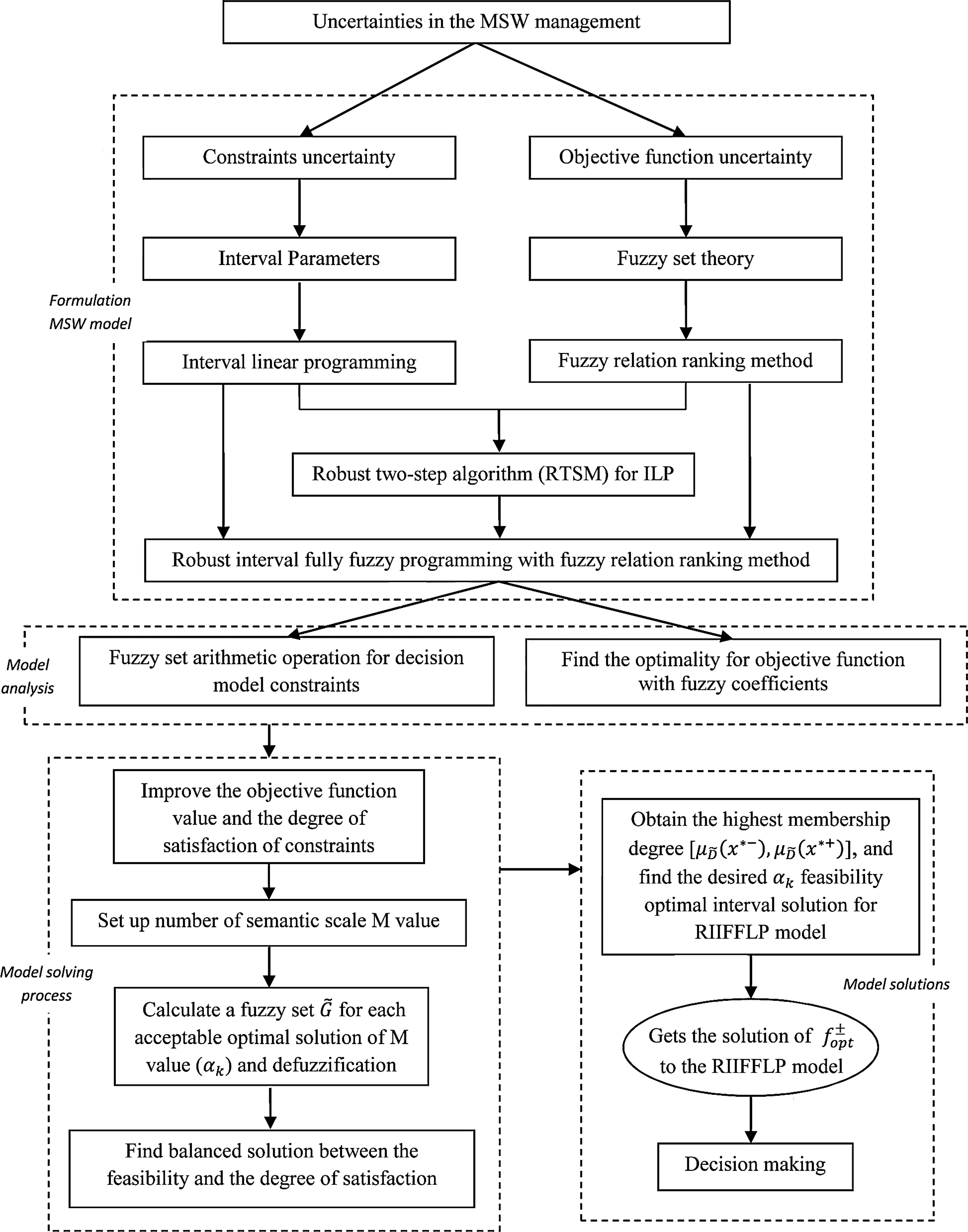
The framework of the RIIFFLP model is presented for analysis in Fig. 1. This programming method considers a system wherein DMs responsible for planning system flows, for example, in water resources projects, municipal treatment works, and public water supply systems, where the fundamental challenge is complex systems that are beyond simple decision-making constructs and are fraught with uncertainty, dissonance, and conflicting information; it can find the minimum system cost under multiple uncertainties.

OPEN IN VIEWER

FIG. 1.

Flow chart of municipal solid waste (MSW) robust interactive interval fully fuzzy linear programming (RIIFFLP) model and solution algorithm.

A Case Study of the Robust Fully Fuzzy Programming

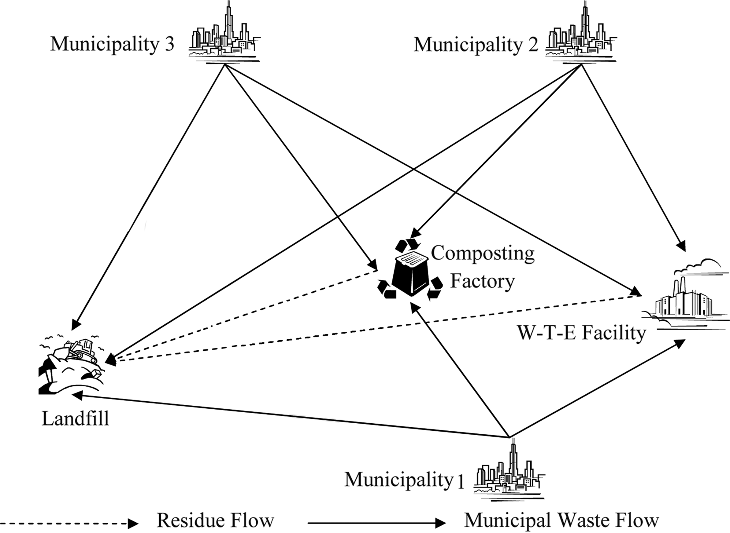
The developed RIIFFLP model is applied to a hypothetical MSW management problem. This hypothetical case presents regional waste planning and facility expansion. It includes three municipalities in which the existing facilities involved include a landfill, a waste-to-energy (WTE) incinerator, and a composting facility to serve the municipality's disposal needs. The planning horizon is 15 years divided into three time periods, with each period having a time interval of 5 years. This MSW system is represented in Fig. 2.

OPEN IN VIEWER

FIG. 2.

Overview of MSW study system.

The waste rate of MSW varies with the population size, influence of the market economy, and time. These uncertain factors cause an interval parameter for the waste generation rate. Table 1 provides cost data for transportation and treatment/disposal for three cities as well as revenue data from WTE and the composting facility. Table 2 contains the fuzzy-random boundary interval of waste generation rate. They indicate that the generation rates are changeable during this long time allocation programming. In Table 3, the capacity expansion option and expansion cost data are listed for the DM. The expansion options are different for each facility. These data are also presented as a fuzzy interval due the regional uncertainty of economic development.

Based on the above analysis of the problem, this MSW system issue can be presented as a question of how to optimize the regional solid waste management system to achieve cost minimization with uncertainties, which means the system coefficients are all fuzzy random interval data. These complex systems can be divided into three subsystems, which are presented in Fig. 2. The allocation strategy requires the minimum value of each subsystem under the total variable waste amount from the three municipalities under a number of environmental capacity constraints. The input of this system is fuzzy boundary interval variables of relative costs, quality of waste flow, and parameters of the objective function. The output is to be an optimal strategy of waste routing for this region. Thus, in this MSW management system, when all parameters are approximated as inexact fuzzy variables, this RIIFFLP method is considered to be a feasible approach to handle this problem. It will also apply the fuzzy relation ranking technique into a fully fuzzy interval linear programming optimized framework.

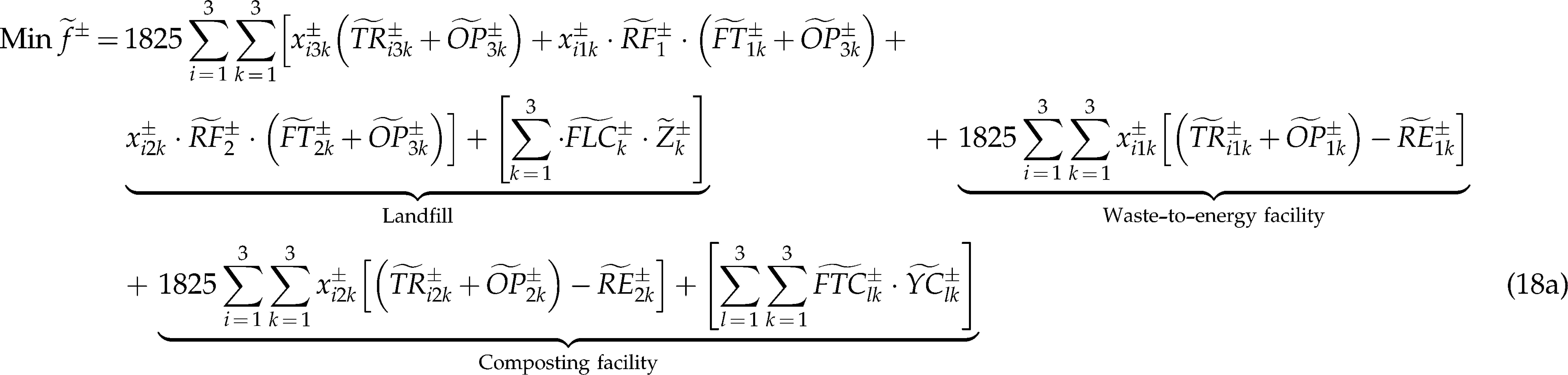
The objective of this problem is to reduce system cost through planning the waste streams to three solid waste processing facilities for the three cities. The parameter i represents cities, the parameter j indicates facilities, and k denotes the different time stages. Thus, the minimum system cost includes three subsystems as, one for each city's waste stream, for each waste management option, including the landfill, the WTE facility, and the composing facility. Every subpart has a minimum system cost requirement. The minimum cost requirement is, therefore, at a minimum, a summation of waste collection/transportation cost and operating costs for each facility. However, the WTE facility and composting facility have revenues from energy prices and fertilizer income. Thus, the objective function can be written as presented in Model (3a) as follows:

OPEN IN VIEWER

Subject to:

(1) WTE facility constraints in each time stage \documentclass{aastex}\usepackage{amsbsy}\usepackage{amsfonts}\usepackage{amssymb}\usepackage{bm}\usepackage{mathrsfs}\usepackage{pifont}\usepackage{stmaryrd}\usepackage{textcomp}\usepackage{portland, xspace}\usepackage{amsmath, amsxtra}\pagestyle{empty}\DeclareMathSizes{10}{9}{7}{6}\begin{document} \begin{align*}\sum\limits_{i = 1}^3 x_{i1k}^{\pm} \leq \widetilde{TW}^{\pm} , \ (k = 1 , 2 , 3) \tag{18{\rm b}}\end{align*} \end{document}

(2) Composting facility capacity constraints in each time stage \documentclass{aastex}\usepackage{amsbsy}\usepackage{amsfonts}\usepackage{amssymb}\usepackage{bm}\usepackage{mathrsfs}\usepackage{pifont}\usepackage{stmaryrd}\usepackage{textcomp}\usepackage{portland, xspace}\usepackage{amsmath, amsxtra}\pagestyle{empty}\DeclareMathSizes{10}{9}{7}{6}\begin{document} \begin{align*}\sum\limits_{i = 1}^3 x_{i2k^{\prime}}^{\pm} - \sum\limits_{l = 1}^3 \sum\limits_{k = 1}^{k^{\prime}} {\widetilde{YC}_{lk}^{\pm}} \cdot {\widetilde{\Delta TC}_l^{\pm}} \leq {\widetilde{TC}^{\pm}} , \quad (k^{\prime} = 1 , 2 , 3) \tag{18{\rm c}}\end{align*} \end{document}

(3) Landfill capacity constraints in each time stage \documentclass{aastex}\usepackage{amsbsy}\usepackage{amsfonts}\usepackage{amssymb}\usepackage{bm}\usepackage{mathrsfs}\usepackage{pifont}\usepackage{stmaryrd}\usepackage{textcomp}\usepackage{portland, xspace}\usepackage{amsmath, amsxtra}\pagestyle{empty}\DeclareMathSizes{10}{9}{7}{6}\begin{document} \begin{align*} \begin{split} & 1825 \sum\limits_{i = 1}^3 \sum\limits_{k = 1}^{k^{\prime}} \left(x_{i3k}^{\pm} + \sum\limits_{j = 1}^2 \widetilde {RF}_j \cdot x_{ijk}^{\pm} \right) - \widetilde{\Delta TL}^{\pm} \\& \cdot \sum \limits_{k = 1}^{k^{\prime}} \widetilde{Z}_k^{\pm} \leq \widetilde{TL}^{\pm} , \quad (k^{\prime} = 1 , 2 , 3)\end{split} \tag{18{\rm d}}\end{align*} \end{document}

(4) Waste generation constraints in each time stage \documentclass{aastex}\usepackage{amsbsy}\usepackage{amsfonts}\usepackage{amssymb}\usepackage{bm}\usepackage{mathrsfs}\usepackage{pifont}\usepackage{stmaryrd}\usepackage{textcomp}\usepackage{portland, xspace}\usepackage{amsmath, amsxtra}\pagestyle{empty}\DeclareMathSizes{10}{9}{7}{6}\begin{document} \begin{align*}\sum\limits_{i = 1}^2 x_{ijk}^{\pm} \geq \widetilde{WG}_{ik}^{\pm} , \quad \forall i , k \tag{18{\rm e}}\end{align*} \end{document}

(5) The integer constraints \documentclass{aastex}\usepackage{amsbsy}\usepackage{amsfonts}\usepackage{amssymb}\usepackage{bm}\usepackage{mathrsfs}\usepackage{pifont}\usepackage{stmaryrd}\usepackage{textcomp}\usepackage{portland, xspace}\usepackage{amsmath, amsxtra}\pagestyle{empty}\DeclareMathSizes{10}{9}{7}{6}\begin{document} \begin{align*} \sum\limits_{l = 1}^3 \widetilde{YC}_{lk}^{\pm}\leq 1 , \quad \forall\ k \tag{18{\rm f}} \end{align*} \end{document} \documentclass{aastex}\usepackage{amsbsy}\usepackage{amsfonts}\usepackage{amssymb}\usepackage{bm}\usepackage{mathrsfs}\usepackage{pifont}\usepackage{stmaryrd}\usepackage{textcomp}\usepackage{portland, xspace}\usepackage{amsmath, amsxtra}\pagestyle{empty}\DeclareMathSizes{10}{9}{7}{6}\begin{document} \begin{align*} \sum\limits_{k = 1}^3 \widetilde{Z}_k^{\pm} \leq 1 , \quad (k = 1 , 2 , 3) \tag{18{\rm g}} \end{align*} \end{document} \documentclass{aastex}\usepackage{amsbsy}\usepackage{amsfonts}\usepackage{amssymb}\usepackage{bm}\usepackage{mathrsfs}\usepackage{pifont}\usepackage{stmaryrd}\usepackage{textcomp}\usepackage{portland, xspace}\usepackage{amsmath, amsxtra}\pagestyle{empty}\DeclareMathSizes{10}{9}{7}{6}\begin{document} \begin{align*}\widetilde{YC}_{lk}^{\pm} \leq1 , \quad \forall l , k \tag{18{\rm h}}\end{align*} \end{document} \documentclass{aastex}\usepackage{amsbsy}\usepackage{amsfonts}\usepackage{amssymb}\usepackage{bm}\usepackage{mathrsfs}\usepackage{pifont}\usepackage{stmaryrd}\usepackage{textcomp}\usepackage{portland, xspace}\usepackage{amsmath, amsxtra}\pagestyle{empty}\DeclareMathSizes{10}{9}{7}{6}\begin{document} \begin{align*}\widetilde {Z}_k^{\pm} \leq 1 , \quad \forall \ k \tag{18{\rm i}}\end{align*} \end{document}

(6) Non-negativity and technical constraints \documentclass{aastex}\usepackage{amsbsy}\usepackage{amsfonts}\usepackage{amssymb}\usepackage{bm}\usepackage{mathrsfs}\usepackage{pifont}\usepackage{stmaryrd}\usepackage{textcomp}\usepackage{portland, xspace}\usepackage{amsmath, amsxtra}\pagestyle{empty}\DeclareMathSizes{10}{9}{7}{6}\begin{document} \begin{align*}x_{ijk}^{\pm} \geq 0 , \quad \forall i , j , k \tag{18{\rm j}}\end{align*} \end{document} \documentclass{aastex}\usepackage{amsbsy}\usepackage{amsfonts}\usepackage{amssymb}\usepackage{bm}\usepackage{mathrsfs}\usepackage{pifont}\usepackage{stmaryrd}\usepackage{textcomp}\usepackage{portland, xspace}\usepackage{amsmath, amsxtra}\pagestyle{empty}\DeclareMathSizes{10}{9}{7}{6}\begin{document} \begin{align*}\widetilde {YC}_{lk}^{\pm} \geq 0 , \quad \forall l , \ k \tag{18{\rm k}}\end{align*} \end{document} \documentclass{aastex}\usepackage{amsbsy}\usepackage{amsfonts}\usepackage{amssymb}\usepackage{bm}\usepackage{mathrsfs}\usepackage{pifont}\usepackage{stmaryrd}\usepackage{textcomp}\usepackage{portland, xspace}\usepackage{amsmath, amsxtra}\pagestyle{empty}\DeclareMathSizes{10}{9}{7}{6}\begin{document} \begin{align*}\widetilde {Z}_k^{\pm} \geq 0 , \quad \forall \ k \tag{18{\rm l}}\end{align*} \end{document}

where \documentclass{aastex}\usepackage{amsbsy}\usepackage{amsfonts}\usepackage{amssymb}\usepackage{bm}\usepackage{mathrsfs}\usepackage{pifont}\usepackage{stmaryrd}\usepackage{textcomp}\usepackage{portland, xspace}\usepackage{amsmath, amsxtra}\pagestyle{empty}\DeclareMathSizes{10}{9}{7}{6}\begin{document} $$\widetilde{f}^{\pm}$$ \end{document} is the objective function value and i is an index for the three municipalities (i=1, 2, 3); j is an index for the facilities (j=1 for WTE facility, j=2 for the composting facility, j=3 for the landfill); k is an index for time periods (k=1, 2, 3); l is also an index for the facility capacity expansion type (l=1, 2, 3); \documentclass{aastex}\usepackage{amsbsy}\usepackage{amsfonts}\usepackage{amssymb}\usepackage{bm}\usepackage{mathrsfs}\usepackage{pifont}\usepackage{stmaryrd}\usepackage{textcomp}\usepackage{portland, xspace}\usepackage{amsmath, amsxtra}\pagestyle{empty}\DeclareMathSizes{10}{9}{7}{6}\begin{document} $$\widetilde{TR}_{ijk}^{\pm}$$ \end{document} represents the waste transportation costs from municipality i to facility j in period k ($/ton); \documentclass{aastex}\usepackage{amsbsy}\usepackage{amsfonts}\usepackage{amssymb}\usepackage{bm}\usepackage{mathrsfs}\usepackage{pifont}\usepackage{stmaryrd}\usepackage{textcomp}\usepackage{portland, xspace}\usepackage{amsmath, amsxtra}\pagestyle{empty}\DeclareMathSizes{10}{9}{7}{6}\begin{document} $$\widetilde{OP}_{jk}^{\pm}$$ \end{document} indicates the operating costs of facility j in period k ($/ton); \documentclass{aastex}\usepackage{amsbsy}\usepackage{amsfonts}\usepackage{amssymb}\usepackage{bm}\usepackage{mathrsfs}\usepackage{pifont}\usepackage{stmaryrd}\usepackage{textcomp}\usepackage{portland, xspace}\usepackage{amsmath, amsxtra}\pagestyle{empty}\DeclareMathSizes{10}{9}{7}{6}\begin{document} $$\widetilde{FLC}_{k}^{\pm}$$ \end{document} denotes the unit capacity expansion cost for the landfill in period k ($/ton); \documentclass{aastex}\usepackage{amsbsy}\usepackage{amsfonts}\usepackage{amssymb}\usepackage{bm}\usepackage{mathrsfs}\usepackage{pifont}\usepackage{stmaryrd}\usepackage{textcomp}\usepackage{portland, xspace}\usepackage{amsmath, amsxtra}\pagestyle{empty}\DeclareMathSizes{10}{9}{7}{6}\begin{document} $$\widetilde{FTC}_{lk}^{\pm}$$ \end{document} is the unit cost of capacity expansion type l for the composting facility in period k ($/ton); \documentclass{aastex}\usepackage{amsbsy}\usepackage{amsfonts}\usepackage{amssymb}\usepackage{bm}\usepackage{mathrsfs}\usepackage{pifont}\usepackage{stmaryrd}\usepackage{textcomp}\usepackage{portland, xspace}\usepackage{amsmath, amsxtra}\pagestyle{empty}\DeclareMathSizes{10}{9}{7}{6}\begin{document} $$\widetilde{RF}_{j}^{\pm}$$ \end{document} indicates the residue flow rates from facility j to the landfill facility (% of incoming mass to WTE facility; j=1, 2); \documentclass{aastex}\usepackage{amsbsy}\usepackage{amsfonts}\usepackage{amssymb}\usepackage{bm}\usepackage{mathrsfs}\usepackage{pifont}\usepackage{stmaryrd}\usepackage{textcomp}\usepackage{portland, xspace}\usepackage{amsmath, amsxtra}\pagestyle{empty}\DeclareMathSizes{10}{9}{7}{6}\begin{document} $$\widetilde{FT}_{jk}^{\pm}$$ \end{document} shows the transportation costs of flow from WTE facility (j=1) and composting facility (j=2) to the landfill facility in period k ($/ton; k=1, 2, 3); \documentclass{aastex}\usepackage{amsbsy}\usepackage{amsfonts}\usepackage{amssymb}\usepackage{bm}\usepackage{mathrsfs}\usepackage{pifont}\usepackage{stmaryrd}\usepackage{textcomp}\usepackage{portland, xspace}\usepackage{amsmath, amsxtra}\pagestyle{empty}\DeclareMathSizes{10}{9}{7}{6}\begin{document} $$\widetilde{RE}_{jk}^{\pm}$$ \end{document} is the revenue from the WTE facility (j=1) and composting facility (j=2) in period k ($/ton; k=1,2,3); \documentclass{aastex}\usepackage{amsbsy}\usepackage{amsfonts}\usepackage{amssymb}\usepackage{bm}\usepackage{mathrsfs}\usepackage{pifont}\usepackage{stmaryrd}\usepackage{textcomp}\usepackage{portland, xspace}\usepackage{amsmath, amsxtra}\pagestyle{empty}\DeclareMathSizes{10}{9}{7}{6}\begin{document} $$\widetilde{TL}^{\pm}$$ \end{document} represents the capacity of the landfill facility (ton); \documentclass{aastex}\usepackage{amsbsy}\usepackage{amsfonts}\usepackage{amssymb}\usepackage{bm}\usepackage{mathrsfs}\usepackage{pifont}\usepackage{stmaryrd}\usepackage{textcomp}\usepackage{portland, xspace}\usepackage{amsmath, amsxtra}\pagestyle{empty}\DeclareMathSizes{10}{9}{7}{6}\begin{document} $$\widetilde{TW}^{\pm}$$ \end{document} is the maximum treatment capacity of the WTE facility (ton); \documentclass{aastex}\usepackage{amsbsy}\usepackage{amsfonts}\usepackage{amssymb}\usepackage{bm}\usepackage{mathrsfs}\usepackage{pifont}\usepackage{stmaryrd}\usepackage{textcomp}\usepackage{portland, xspace}\usepackage{amsmath, amsxtra}\pagestyle{empty}\DeclareMathSizes{10}{9}{7}{6}\begin{document} $$\widetilde{TC}^{\pm}$$ \end{document} is the maximum treatment capacity of the composting facility (ton); \documentclass{aastex}\usepackage{amsbsy}\usepackage{amsfonts}\usepackage{amssymb}\usepackage{bm}\usepackage{mathrsfs}\usepackage{pifont}\usepackage{stmaryrd}\usepackage{textcomp}\usepackage{portland, xspace}\usepackage{amsmath, amsxtra}\pagestyle{empty}\DeclareMathSizes{10}{9}{7}{6}\begin{document} $$\widetilde{WG}_{jk}^{\pm}$$ \end{document} is the waste generation rate in municipality i in period k; \documentclass{aastex}\usepackage{amsbsy}\usepackage{amsfonts}\usepackage{amssymb}\usepackage{bm}\usepackage{mathrsfs}\usepackage{pifont}\usepackage{stmaryrd}\usepackage{textcomp}\usepackage{portland, xspace}\usepackage{amsmath, amsxtra}\pagestyle{empty}\DeclareMathSizes{10}{9}{7}{6}\begin{document} $$x_{ijk}^{\pm}$$ \end{document} represents the waste flow from municipality j to facility i in period k (ton/day); \documentclass{aastex}\usepackage{amsbsy}\usepackage{amsfonts}\usepackage{amssymb}\usepackage{bm}\usepackage{mathrsfs}\usepackage{pifont}\usepackage{stmaryrd}\usepackage{textcomp}\usepackage{portland, xspace}\usepackage{amsmath, amsxtra}\pagestyle{empty}\DeclareMathSizes{10}{9}{7}{6}\begin{document} $$\widetilde{YC}_{jk}^{\pm}$$ \end{document} is an integer variable for the lth expansion of the composting facility in period k; \documentclass{aastex}\usepackage{amsbsy}\usepackage{amsfonts}\usepackage{amssymb}\usepackage{bm}\usepackage{mathrsfs}\usepackage{pifont}\usepackage{stmaryrd}\usepackage{textcomp}\usepackage{portland, xspace}\usepackage{amsmath, amsxtra}\pagestyle{empty}\DeclareMathSizes{10}{9}{7}{6}\begin{document} $$\widetilde{Z}_{k}^{\pm}$$ \end{document} is an integer variable for the lth expansion of the landfill in period k; \documentclass{aastex}\usepackage{amsbsy}\usepackage{amsfonts}\usepackage{amssymb}\usepackage{bm}\usepackage{mathrsfs}\usepackage{pifont}\usepackage{stmaryrd}\usepackage{textcomp}\usepackage{portland, xspace}\usepackage{amsmath, amsxtra}\pagestyle{empty}\DeclareMathSizes{10}{9}{7}{6}\begin{document} $$\widetilde{\Delta TL}^{\pm}$$ \end{document} is the amount of expansion capacity for the landfill (ton); \documentclass{aastex}\usepackage{amsbsy}\usepackage{amsfonts}\usepackage{amssymb}\usepackage{bm}\usepackage{mathrsfs}\usepackage{pifont}\usepackage{stmaryrd}\usepackage{textcomp}\usepackage{portland, xspace}\usepackage{amsmath, amsxtra}\pagestyle{empty}\DeclareMathSizes{10}{9}{7}{6}\begin{document} $$\widetilde{\Delta TC}_l^{\pm}$$ \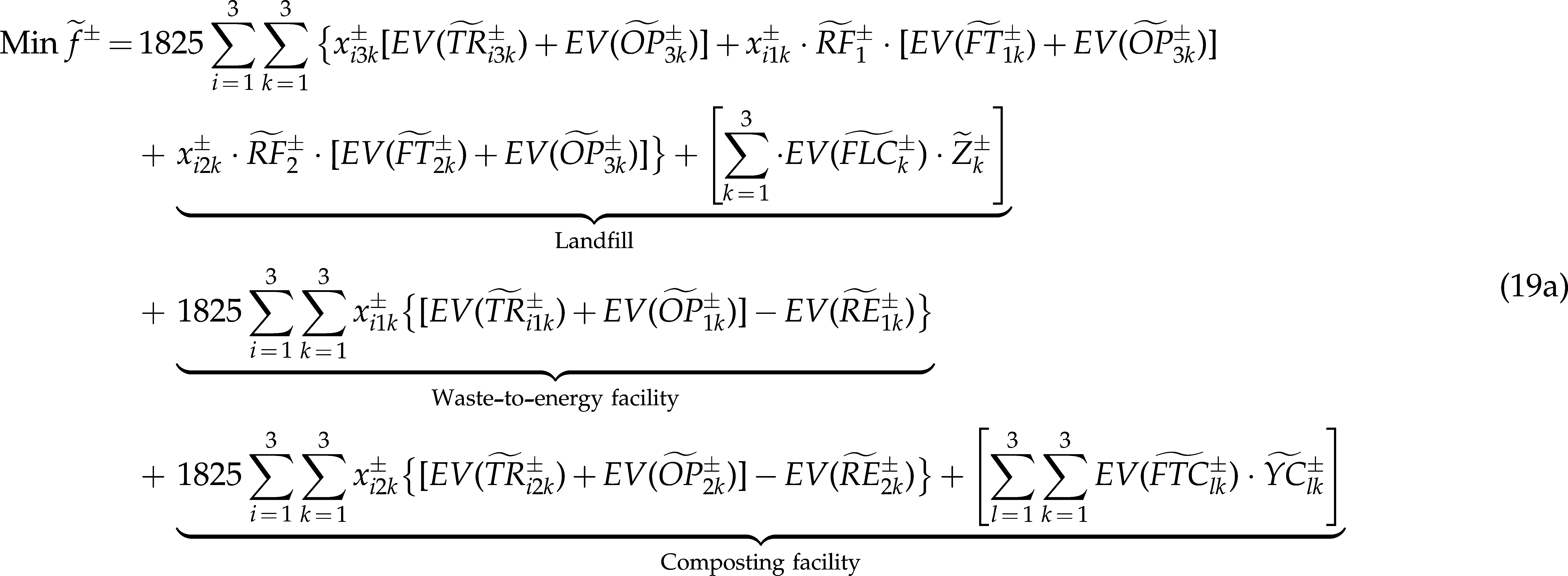end{document} is the amount of the lth type of expansion capacity for the composting facility (ton). Thus, based on the RIIFFLP algorithm, Model (18) can be solved with an RTSM, which corresponds to Fan's algorithm (Fan and Huang, 2011). Model (18) can be rewritten as follows:

OPEN IN VIEWER

Subject to: \documentclass{aastex}\usepackage{amsbsy}\usepackage{amsfonts}\usepackage{amssymb}\usepackage{bm}\usepackage{mathrsfs}\usepackage{pifont}\usepackage{stmaryrd}\usepackage{textcomp}\usepackage{portland, xspace}\usepackage{amsmath, amsxtra}\pagestyle{empty}\DeclareMathSizes{10}{9}{7}{6}\begin{document} \begin{align*} \sum_{i = 1}^3 x_{i1k^{\prime}}^{\pm} \leq \alpha E_1^{TW^{\pm}} + (1 - \alpha) E_2^{TW^{\pm}} , \quad (k^{\prime} = 1 , 2 , 3) \tag{19{\rm b}} \end{align*} \end{document} \documentclass{aastex}\usepackage{amsbsy}\usepackage{amsfonts}\usepackage{amssymb}\usepackage{bm}\usepackage{mathrsfs}\usepackage{pifont}\usepackage{stmaryrd}\usepackage{textcomp}\usepackage{portland, xspace}\usepackage{amsmath, amsxtra}\pagestyle{empty}\DeclareMathSizes{10}{9}{7}{6}\begin{document} \begin{align*} \begin{split} \sum_{i = 1}^3 x_{i2k^{\prime}}^{\pm} - \sum_{l = 1}^3 \sum_{k = 1}^{k^{\prime}} \left[(1 - \alpha) E_1^{\Delta TC_l^{\pm}} + \alpha E_2^{\Delta TC_l^{\pm}} \right] \cdot \widetilde{YC}_{lk}^{\pm} \leq \alpha E_1^{TC^{\pm}} \\\quad+ (1 - \alpha) E_2^{TC^{\pm}} , \quad (k^{\prime} = 1 , 2 , 3)\end{split} \tag{19{\rm c}}\end{align*} \end{document} \documentclass{aastex}\usepackage{amsbsy}\usepackage{amsfonts}\usepackage{amssymb}\usepackage{bm}\usepackage{mathrsfs}\usepackage{pifont}\usepackage{stmaryrd}\usepackage{textcomp}\usepackage{portland, xspace}\usepackage{amsmath, amsxtra}\pagestyle{empty}\DeclareMathSizes{10}{9}{7}{6}\begin{document} \begin{align*} \begin{split} & 1825 \sum_{i = 1}^3 \sum_{k = 1}^{k^{\prime}} \left(x_{i3k}^{\pm} + \sum_{j = 2}^3 ((1 - \alpha) E_1^{RF_j^{\pm}} + \alpha E_2^{RF_j^{\pm}}) \cdot x_{ijk}^{\pm} \right) \\ & \quad- ((1 - \alpha) E_1^{\Delta TL^{\pm}} + \alpha E_2^{\Delta TL^{\pm}})) \cdot \sum_{k = 1}^{k^{\prime}} \widetilde{Z}_k^{\pm} \\ & \quad \leq \alpha E_1^{TL ^{\pm}} + (1 - \alpha) E_2^{TL^{\pm}} , \quad (k^{\prime} = 1 , 2 , 3)\end{split} \tag{19{\rm d}}\end{align*} \end{document} \documentclass{aastex}\usepackage{amsbsy}\usepackage{amsfonts}\usepackage{amssymb}\usepackage{bm}\usepackage{mathrsfs}\usepackage{pifont}\usepackage{stmaryrd}\usepackage{textcomp}\usepackage{portland, xspace}\usepackage{amsmath, amsxtra}\pagestyle{empty}\DeclareMathSizes{10}{9}{7}{6}\begin{document} \begin{align*}\sum_{i = 1}^3 x_{ijk}^{\pm} \geq \alpha E_2^{WG_{ik}^{\pm}} + (1 - \alpha) E_1^{WG_{ik}^{\pm}} , \quad \forall j , k \tag{19{\rm e}}\end{align*} \end{document} \documentclass{aastex}\usepackage{amsbsy}\usepackage{amsfonts}\usepackage{amssymb}\usepackage{bm}\usepackage{mathrsfs}\usepackage{pifont}\usepackage{stmaryrd}\usepackage{textcomp}\usepackage{portland, xspace}\usepackage{amsmath, amsxtra}\pagestyle{empty}\DeclareMathSizes{10}{9}{7}{6}\begin{document} \begin{align*}x_{ijkopt}^ + \geq x_{ijk}^ - , \quad \forall i , j , k \tag{19{\rm f}}\end{align*} \end{document} \documentclass{aastex}\usepackage{amsbsy}\usepackage{amsfonts}\usepackage{amssymb}\usepackage{bm}\usepackage{mathrsfs}\usepackage{pifont}\usepackage{stmaryrd}\usepackage{textcomp}\usepackage{portland, xspace}\usepackage{amsmath, amsxtra}\pagestyle{empty}\DeclareMathSizes{10}{9}{7}{6}\begin{document} \begin{align*}YC_{lkopt}^ + \geq YC_{lk}^ - , \quad \forall l , k \tag{19{\rm g}}\end{align*} \end{document} \documentclass{aastex}\usepackage{amsbsy}\usepackage{amsfonts}\usepackage{amssymb}\usepackage{bm}\usepackage{mathrsfs}\usepackage{pifont}\usepackage{stmaryrd}\usepackage{textcomp}\usepackage{portland, xspace}\usepackage{amsmath, amsxtra}\pagestyle{empty}\DeclareMathSizes{10}{9}{7}{6}\begin{document} \begin{align*}Z_{kopt}^ + \geq Z_k^ - , \quad \forall \ k \tag{19{\rm h}}\end{align*} \end{document} \documentclass{aastex}\usepackage{amsbsy}\usepackage{amsfonts}\usepackage{amssymb}\usepackage{bm}\usepackage{mathrsfs}\usepackage{pifont}\usepackage{stmaryrd}\usepackage{textcomp}\usepackage{portland, xspace}\usepackage{amsmath, amsxtra}\pagestyle{empty}\DeclareMathSizes{10}{9}{7}{6}\begin{document} \begin{align*}\sum_{l = 1}^3 \widetilde{YC}_{lk}^{\pm} \leq 1 , \quad \forall \ k \tag{19{\rm i}}\end{align*} \end{document} \documentclass{aastex}\usepackage{amsbsy}\usepackage{amsfonts}\usepackage{amssymb}\usepackage{bm}\usepackage{mathrsfs}\usepackage{pifont}\usepackage{stmaryrd}\usepackage{textcomp}\usepackage{portland, xspace}\usepackage{amsmath, amsxtra}\pagestyle{empty}\DeclareMathSizes{10}{9}{7}{6}\begin{document} \begin{align*}\sum_{k = 1}^3 \widetilde{Z}_k^{\pm} \leq 1 , \quad (k = 1 , 2 , 3) \tag{19{\rm j}}\end{align*} \end{document} \documentclass{aastex}\usepackage{amsbsy}\usepackage{amsfonts}\usepackage{amssymb}\usepackage{bm}\usepackage{mathrsfs}\usepackage{pifont}\usepackage{stmaryrd}\usepackage{textcomp}\usepackage{portland, xspace}\usepackage{amsmath, amsxtra}\pagestyle{empty}\DeclareMathSizes{10}{9}{7}{6}\begin{document} \begin{align*}\widetilde{YC}_{lk}^{\pm} \leq 1 , \quad \forall l , k \tag{19{\rm k}}\end{align*} \end{document} \documentclass{aastex}\usepackage{amsbsy}\usepackage{amsfonts}\usepackage{amssymb}\usepackage{bm}\usepackage{mathrsfs}\usepackage{pifont}\usepackage{stmaryrd}\usepackage{textcomp}\usepackage{portland, xspace}\usepackage{amsmath, amsxtra}\pagestyle{empty}\DeclareMathSizes{10}{9}{7}{6}\begin{document} \begin{align*}\widetilde{Z}_k^{\pm} \leq 1 , \quad \forall \ k \tag{19{\rm l}}\end{align*} \end{document} \documentclass{aastex}\usepackage{amsbsy}\usepackage{amsfonts}\usepackage{amssymb}\usepackage{bm}\usepackage{mathrsfs}\usepackage{pifont}\usepackage{stmaryrd}\usepackage{textcomp}\usepackage{portland, xspace}\usepackage{amsmath, amsxtra}\pagestyle{empty}\DeclareMathSizes{10}{9}{7}{6}\begin{document} \begin{align*}x_{ijk}^{\pm} \geq 0 , \quad \forall i , j , k \tag{19{\rm m}}\end{align*} \end{document} \documentclass{aastex}\usepackage{amsbsy}\usepackage{amsfonts}\usepackage{amssymb}\usepackage{bm}\usepackage{mathrsfs}\usepackage{pifont}\usepackage{stmaryrd}\usepackage{textcomp}\usepackage{portland, xspace}\usepackage{amsmath, amsxtra}\pagestyle{empty}\DeclareMathSizes{10}{9}{7}{6}\begin{document} \begin{align*}\widetilde{YC}_{lk}^{\pm} \geq 0 , \quad \forall l , k \tag{19{\rm n}}\end{align*} \end{document} \documentclass{aastex}\usepackage{amsbsy}\usepackage{amsfonts}\usepackage{amssymb}\usepackage{bm}\usepackage{mathrsfs}\usepackage{pifont}\usepackage{stmaryrd}\usepackage{textcomp}\usepackage{portland, xspace}\usepackage{amsmath, amsxtra}\pagestyle{empty}\DeclareMathSizes{10}{9}{7}{6}\begin{document} \begin{align*}\widetilde{Z}_k^{\pm} \geq 0 , \quad \forall \ k \tag{19{\rm o}}\end{align*} \end{document}

By solving Model (19), the α_k-acceptable optimal solution will be achieved for each α_k. However, to obtain the final decision plan, it is necessary to set up a fuzzy set \documentclass{aastex}\usepackage{amsbsy}\usepackage{amsfonts}\usepackage{amssymb}\usepackage{bm}\usepackage{mathrsfs}\usepackage{pifont}\usepackage{stmaryrd}\usepackage{textcomp}\usepackage{portland, xspace}\usepackage{amsmath, amsxtra}\pagestyle{empty}\DeclareMathSizes{10}{9}{7}{6}\begin{document} $$\widetilde {G}$$ \end{document} for each α_k solution and calculate the membership value of each fuzzy set \documentclass{aastex}\usepackage{amsbsy}\usepackage{amsfonts}\usepackage{amssymb}\usepackage{bm}\usepackage{mathrsfs}\usepackage{pifont}\usepackage{stmaryrd}\usepackage{textcomp}\usepackage{portland, xspace}\usepackage{amsmath, amsxtra}\pagestyle{empty}\DeclareMathSizes{10}{9}{7}{6}\begin{document} $$\tilde{f}^0 (\alpha_k)$$ \end{document} to find the optimal balance between the feasibility degree and the degree of satisfaction. At this point, the desired α_k feasibility optimal interval solution can be obtained for the solid waste management function as \documentclass{aastex}\usepackage{amsbsy}\usepackage{amsfonts}\usepackage{amssymb}\usepackage{bm}\usepackage{mathrsfs}\usepackage{pifont}\usepackage{stmaryrd}\usepackage{textcomp}\usepackage{portland, xspace}\usepackage{amsmath, amsxtra}\pagestyle{empty}\DeclareMathSizes{10}{9}{7}{6}\begin{document} $$[\mu_{\tilde{D}} (x^{*+}) , \mu_{\tilde{D}} (x^{*-})]$$ \end{document} .

Result Analysis

With a series of calculations, the results of the waste flow for this solid waste management system can be obtained as shown in Table 4 for different α feasibility degrees. The six α degrees that the DMs would be willing to accept were considered. From the solution from the RIIFFLP model, the nonzero waste flows are listed in Table 4, along with the optimized system costs. Similarly, this table also represents other waste flows clearly, when the special α levels are applied to the system. In addition, Table 4 illustrates that the treatment capacity of the landfill facility will increase as time progresses. It also shows that the compositing facility can maintain a certain quantity of waste flow in each 5-year stage; however, the waste flows allocated to the WTE facility are reduced. For this same reason, it eventually will no longer be waste, transported to the WTE. This demonstrates that different combinative considerations regarding a wide variety of inputs can lead to an optimized waste flow allocation pattern. These interval solutions do not only indicate the movements of waste flow, but reflect the uncertainties in planning situations. Finally, with respect to these waste flows, the expansion options are presented in Table 5, in which, the items tabulated are also influenced by different α feasible degrees.

Table 5 presents the results of expansions of the landfill and composting facilities. It represents the optimal strategies of expansion. Those options can promise an optimal result for this solid waste management system. They lead to low system costs with relatively low risk.

Table 6 represents the different feasibility degrees, which would yield varied systems cost, and result in different waste flow allocation patterns. The minimum system costs would be $[(219,773,300; 226,231,800; and 227,338,600), (389,686,800; 399,811,000; and 410,056,100)]. The results reveal two conflicting factors between systems cost and constraint violation. If the DMs plan to obtain a maximum satisfaction degree, this obligation can lead to a lower level of constraint feasibility degree to be achieved; in other words, a better constraint feasibility degree corresponds to a lower degree of satisfaction.

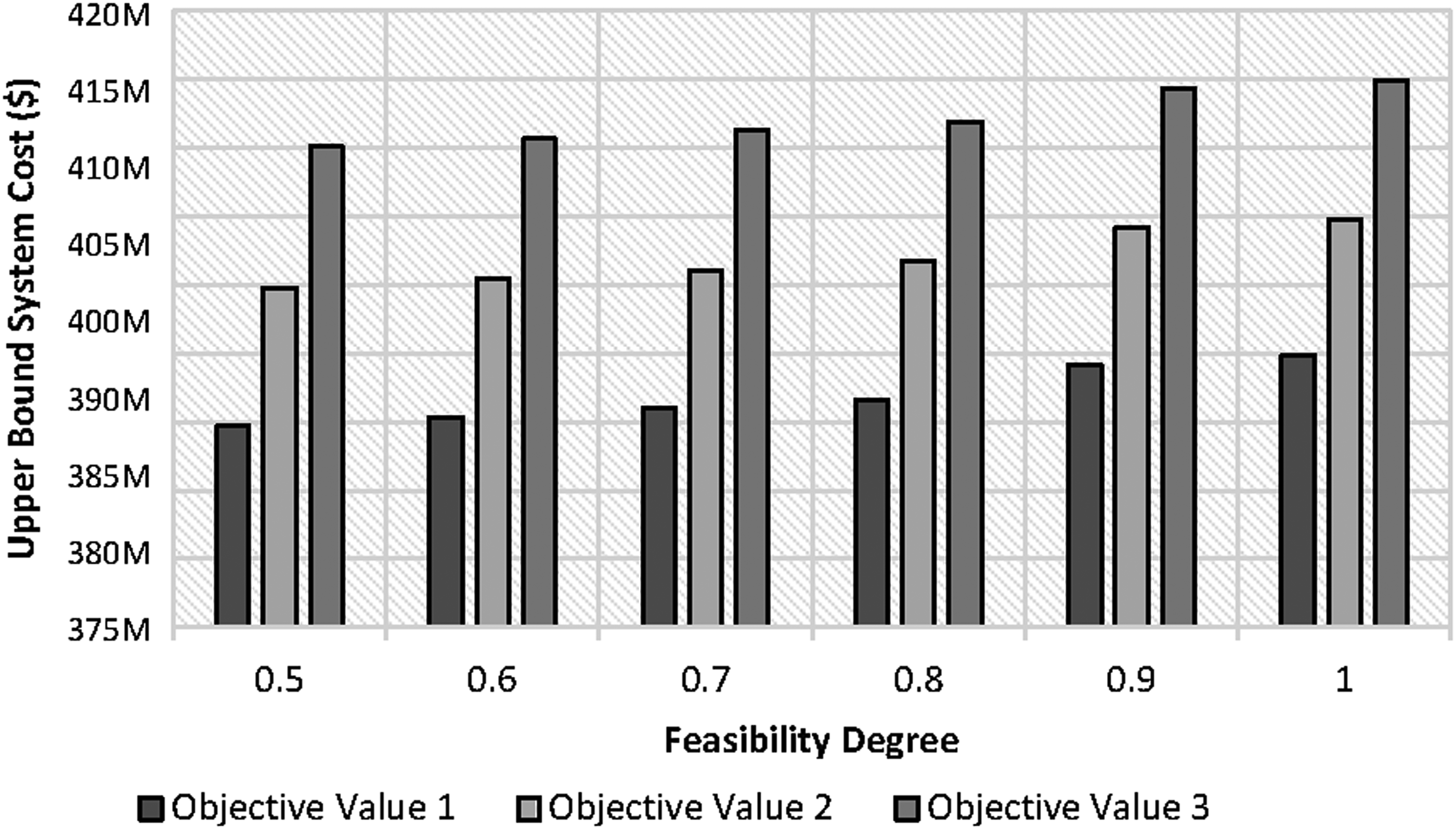
Figure 3 shows the upper fuzzy bound interval cost for six α levels. Figure 4 presents the lower fuzzy bound interval cost for the same six α levels. Figure 5 illustrates the interval fuzzy bounds reference as systems cost. The solutions indicate that the systems cost steadily increase by using the higher α feasibility. It also suggests that a looser constraint feasibility should relate to a lower systems cost. Therefore, the DMs have to identify a good balance between constraint feasibility and systems final goal in real solid waste management problems.

OPEN IN VIEWER

FIG. 3.

Upper bound system cost for waste management under uncertainty.

OPEN IN VIEWER

FIG. 4.

Lower bound system cost for waste management under uncertainty.

OPEN IN VIEWER

FIG. 5.

Interval objective costs for waste management under uncertainty.

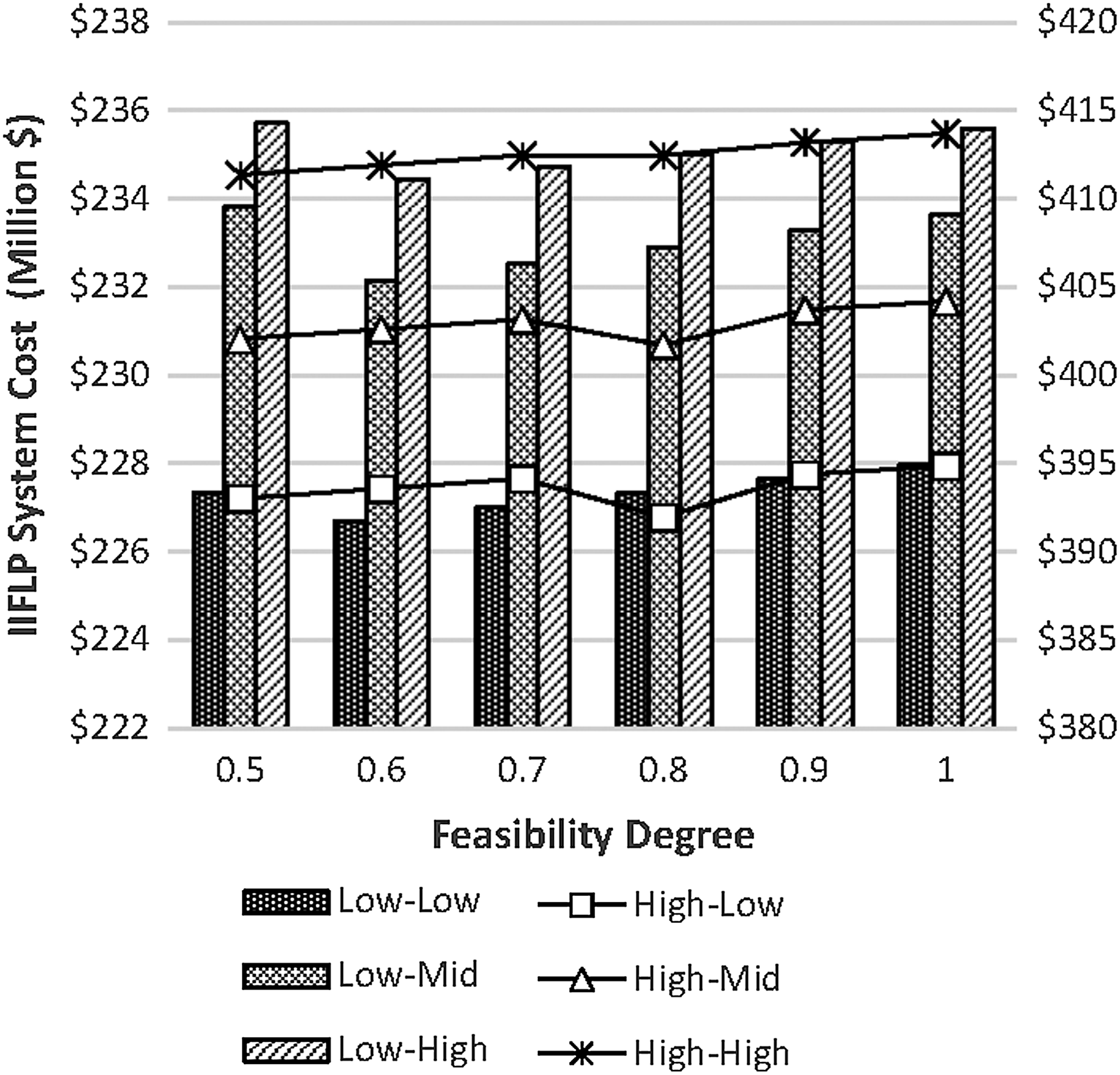
To get a balanced solution between the feasibility degree and the satisfaction degree, managers would be asked to specify a low cost goal \documentclass{aastex}\usepackage{amsbsy}\usepackage{amsfonts}\usepackage{amssymb}\usepackage{bm}\usepackage{mathrsfs}\usepackage{pifont}\usepackage{stmaryrd}\usepackage{textcomp}\usepackage{portland, xspace}\usepackage{amsmath, amsxtra}\pagestyle{empty}\DeclareMathSizes{10}{9}{7}{6}\begin{document} $$\overline {G}$$ \end{document} and its tolerance threshold \documentclass{aastex}\usepackage{amsbsy}\usepackage{amsfonts}\usepackage{amssymb}\usepackage{bm}\usepackage{mathrsfs}\usepackage{pifont}\usepackage{stmaryrd}\usepackage{textcomp}\usepackage{portland, xspace}\usepackage{amsmath, amsxtra}\pagestyle{empty}\DeclareMathSizes{10}{9}{7}{6}\begin{document} $$\underline{G}$$ \end{document} , which can be expressed as a fuzzy set ( \documentclass{aastex}\usepackage{amsbsy}\usepackage{amsfonts}\usepackage{amssymb}\usepackage{bm}\usepackage{mathrsfs}\usepackage{pifont}\usepackage{stmaryrd}\usepackage{textcomp}\usepackage{portland, xspace}\usepackage{amsmath, amsxtra}\pagestyle{empty}\DeclareMathSizes{10}{9}{7}{6}\begin{document} $$\widetilde {G}$$ \end{document} ). Table 7 shows lower and upper bounds of the satisfaction degree of the fuzzy goal under each α-acceptable system cost. If the t-norm algebraic constraint is considered, the membership degree of each α-acceptable optimal solution \documentclass{aastex}\usepackage{amsbsy}\usepackage{amsfonts}\usepackage{amssymb}\usepackage{bm}\usepackage{mathrsfs}\usepackage{pifont}\usepackage{stmaryrd}\usepackage{textcomp}\usepackage{portland, xspace}\usepackage{amsmath, amsxtra}\pagestyle{empty}\DeclareMathSizes{10}{9}{7}{6}\begin{document} $$\widetilde{D}$$ \end{document} (the fuzzy set that represents the balance between the feasibility degree of constraints and satisfaction degree of the fuzzy goal) would be achieved. In Table 7, the solution with 0.9 feasibility should be the optimal solution for this case because it has the lowest deviation value. Therefore, the optimal cost of this solid waste management should be obtained at $(230,408,400; 401,710,800). This feasible solution provided by the RIIFFLP model reflects various uncertainties of the solid waste management as well as the compromise of both constraints and objective function.

Discussion

In this study, a new RIIFFLP model has been established for solid waste management. Through the above results, the optimum cost value of this MSW optimum value can be found $(230,408,400; 401,710,800) at α=0.9. It should be chosen as the acceptable level of satisfaction for both constraints and objective value. This MSW management problem can also be solved through interactive interval FLP (IIFLP) by calculating the lower bound first without the RTSM, which can fix decision solutions under the best-case constraints. Table 8 shows the solution obtained from the IIFLP model and the RIIFFLP model in comparison.

OPEN IN VIEWER

\documentclass{aastex}\usepackage{amsbsy}\usepackage{amsfonts}\usepackage{amssymb}\usepackage{bm}\usepackage{mathrsfs}\usepackage{pifont}\usepackage{stmaryrd}\usepackage{textcomp}\usepackage{portland, xspace}\usepackage{amsmath, amsxtra}\pagestyle{empty}\DeclareMathSizes{10}{9}{7}{6}\begin{document} \begin{align*}\sum_{i = 1}^3 x_{i1k^{\prime}}^{\pm} \leq \alpha E_1^{TW^{\pm}} + (1 - \alpha) E_2^{TW^{\pm}} , \quad (k^{\prime} = 1 , 2 , 3) \tag{20{\rm b}}\end{align*} \end{document} \documentclass{aastex}\usepackage{amsbsy}\usepackage{amsfonts}\usepackage{amssymb}\usepackage{bm}\usepackage{mathrsfs}\usepackage{pifont}\usepackage{stmaryrd}\usepackage{textcomp}\usepackage{portland, xspace}\usepackage{amsmath, amsxtra}\pagestyle{empty}\DeclareMathSizes{10}{9}{7}{6}\begin{document} \begin{align*} \sum_{i = 1}^3 x_{i2k^{\prime}}^{\pm} - \sum_{l = 1}^3 \sum_{k = 1}^{k^{\prime}} [(1 - \alpha) E_1^{\Delta TC_l^{\pm}} + \alpha E_2^{\Delta TC_l^{\pm}}] \cdot \widetilde{YC}_{lk}^{\pm} \leq \alpha E_1^{TC^{\pm}} + (1 - \alpha) E_2^{TC^{\pm}} , \quad (k^{\prime} = 1 , 2 , 3) \tag{20{\rm c}}\end{align*} \end{document} \documentclass{aastex}\usepackage{amsbsy}\usepackage{amsfonts}\usepackage{amssymb}\usepackage{bm}\usepackage{mathrsfs}\usepackage{pifont}\usepackage{stmaryrd}\usepackage{textcomp}\usepackage{portland, xspace}\usepackage{amsmath, amsxtra}\pagestyle{empty}\DeclareMathSizes{10}{9}{7}{6}\begin{document} \begin{align*} {1825 \sum_{i = 1}^3 \sum_{k = 1}^{k^{\prime}} \Big(x_{i3k}^{\pm} + \sum_{j = 2}^3 ((1 - \alpha) E_1^{RF_j^{\pm}} + \alpha E_2^{RF_j^{\pm}}) \cdot x_{ijk}^{\pm} \Big) - ((1 - \alpha) E_1^{\Delta TL^{\pm}} + \alpha E_2^{\Delta TL^{\pm}})) \cdot \sum_{k = 1}^{k^{\prime}} \widetilde{Z}_k^{\pm}} \, \leq \alpha E_1^{TL ^{\pm}} + (1 - \alpha) E_2^{TL^{\pm}} \quad (k^{\prime} = 1 , 2 , 3) \tag{20{\rm d}}\end{align*} \end{document} \documentclass{aastex}\usepackage{amsbsy}\usepackage{amsfonts}\usepackage{amssymb}\usepackage{bm}\usepackage{mathrsfs}\usepackage{pifont}\usepackage{stmaryrd}\usepackage{textcomp}\usepackage{portland, xspace}\usepackage{amsmath, amsxtra}\pagestyle{empty}\DeclareMathSizes{10}{9}{7}{6}\begin{document} \begin{align*} \sum\limits_{i = 1}^3 x_{ijk}^{\pm} \geq \alpha E_2^{WG_{ik}^{\pm}} + (1 - \alpha) E_1^{WG_{ik}^{\pm}} , \quad \forall j , k \tag{20{\rm e}} \end{align*} \end{document} \documentclass{aastex}\usepackage{amsbsy}\usepackage{amsfonts}\usepackage{amssymb}\usepackage{bm}\usepackage{mathrsfs}\usepackage{pifont}\usepackage{stmaryrd}\usepackage{textcomp}\usepackage{portland, xspace}\usepackage{amsmath, amsxtra}\pagestyle{empty}\DeclareMathSizes{10}{9}{7}{6}\begin{document} \begin{align*}\sum\limits_{l = 1}^3 \widetilde{YC}_{lk}^{\pm} \leq 1 , \quad \forall \ k \tag{20{\rm f}}\end{align*} \end{document} \documentclass{aastex}\usepackage{amsbsy}\usepackage{amsfonts}\usepackage{amssymb}\usepackage{bm}\usepackage{mathrsfs}\usepackage{pifont}\usepackage{stmaryrd}\usepackage{textcomp}\usepackage{portland, xspace}\usepackage{amsmath, amsxtra}\pagestyle{empty}\DeclareMathSizes{10}{9}{7}{6}\begin{document} \begin{align*}\sum\limits_{k = 1}^3 \widetilde{Z}_k^{\pm} \leq 1 , \quad (k = 1 , 2 , 3) \tag{20{\rm g}}\end{align*} \end{document} \documentclass{aastex}\usepackage{amsbsy}\usepackage{amsfonts}\usepackage{amssymb}\usepackage{bm}\usepackage{mathrsfs}\usepackage{pifont}\usepackage{stmaryrd}\usepackage{textcomp}\usepackage{portland, xspace}\usepackage{amsmath, amsxtra}\pagestyle{empty}\DeclareMathSizes{10}{9}{7}{6}\begin{document} \begin{align*}\widetilde{YC}_{lk}^{\pm} \leq 1 , \quad \forall l , k \tag{20{\rm h}}\end{align*} \end{document} \documentclass{aastex}\usepackage{amsbsy}\usepackage{amsfonts}\usepackage{amssymb}\usepackage{bm}\usepackage{mathrsfs}\usepackage{pifont}\usepackage{stmaryrd}\usepackage{textcomp}\usepackage{portland, xspace}\usepackage{amsmath, amsxtra}\pagestyle{empty}\DeclareMathSizes{10}{9}{7}{6}\begin{document} \begin{align*}\widetilde {Z}_k^{\pm} \leq 1 , \quad \forall \ k \tag{20{\rm i}}\end{align*} \end{document} \documentclass{aastex}\usepackage{amsbsy}\usepackage{amsfonts}\usepackage{amssymb}\usepackage{bm}\usepackage{mathrsfs}\usepackage{pifont}\usepackage{stmaryrd}\usepackage{textcomp}\usepackage{portland, xspace}\usepackage{amsmath, amsxtra}\pagestyle{empty}\DeclareMathSizes{10}{9}{7}{6}\begin{document} \begin{align*}x_{ijk}^{\pm} \geq 0 , \quad \forall \ i , j , k \tag{20{\rm j}}\end{align*} \end{document} \documentclass{aastex}\usepackage{amsbsy}\usepackage{amsfonts}\usepackage{amssymb}\usepackage{bm}\usepackage{mathrsfs}\usepackage{pifont}\usepackage{stmaryrd}\usepackage{textcomp}\usepackage{portland, xspace}\usepackage{amsmath, amsxtra}\pagestyle{empty}\DeclareMathSizes{10}{9}{7}{6}\begin{document} \begin{align*}\widetilde{YC}_{lk}^{\pm} \geq 0 , \quad \forall l , k \tag{20{\rm k}}\end{align*} \end{document} \documentclass{aastex}\usepackage{amsbsy}\usepackage{amsfonts}\usepackage{amssymb}\usepackage{bm}\usepackage{mathrsfs}\usepackage{pifont}\usepackage{stmaryrd}\usepackage{textcomp}\usepackage{portland, xspace}\usepackage{amsmath, amsxtra}\pagestyle{empty}\DeclareMathSizes{10}{9}{7}{6}\begin{document} \begin{align*}\widetilde{Z}_k^{\pm} \geq 0 , \quad \forall \ k \tag{20{\rm l}}\end{align*} \end{document}

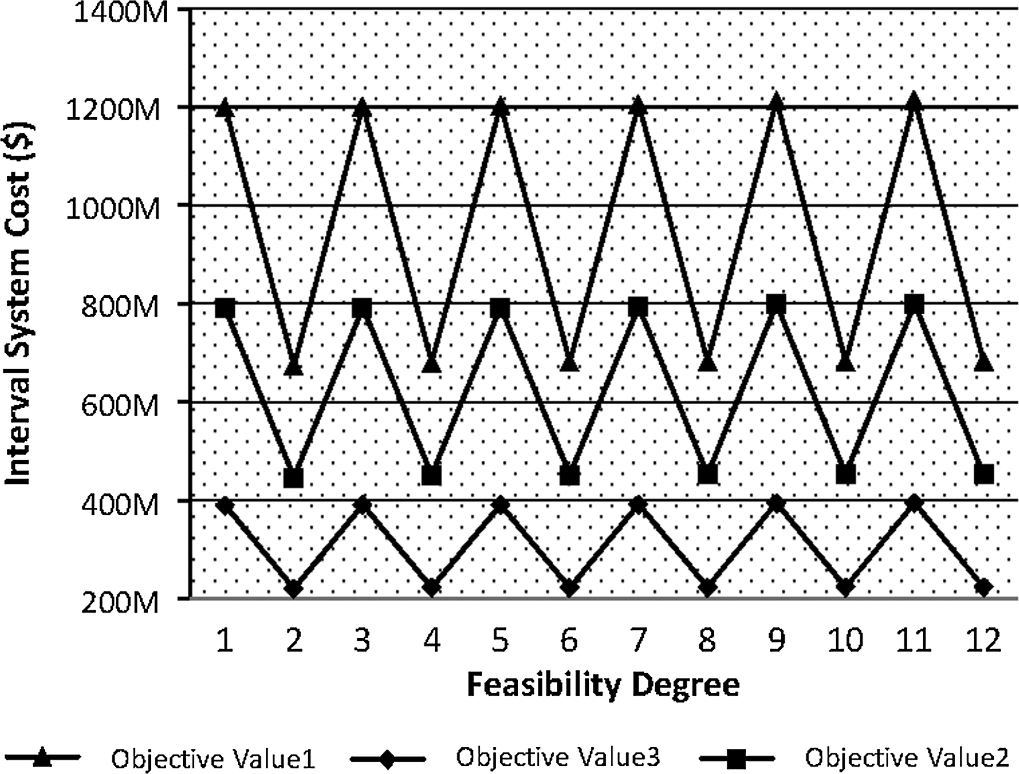
Figures 6 and 7 indicate two results from both the IIFLP and RIIFFLP model under different α levels. Comparing all results, the solutions of RIIFFLP are more accurate than IIFLP. It has a narrower interval range, which indicates a more precise solution. This is the reason the RIIFFLP model can avoid absolute constraint violation as the decision variables fluctuate with the generated decision space. This characteristic of RIIFFLP is very significant because such uncertainties existing in real-world problems can be well reflected. Therefore, the advantages of the RIIFFLP model are significant.

OPEN IN VIEWER

FIG. 6.

Solutions of interactive interval fuzzy linear programming (IIFLP) for waste management under uncertainty.

OPEN IN VIEWER

FIG. 7.

Solutions of robust IIFLP (RIIFLP) for waste management under uncertainty.

Conclusions

In this study, the RIIFFLP approach has been introduced into modeling of MSW management. This method can handle the more complex uncertainty that exists in systems, such as the interval fuzzy parameters. It has improved the fuzzy objective function value and the degree of the constraint requirements. In the future, it can be applied to many other environmental problems such as air pollution management and water resource management. It is recommended that an alternative fuzzy ranking method be used to reduce the complex defuzzification process, and it should also be applied to a real-world problem for further evaluation.

Further Reading

In addition to those works cited previously, readers are directed to other helpful sources in the literature (Huang et al., 2001a, 2001b; Van Hop, 2007; Li et al., 2007, 2008; Cai et al., 2009; Guo et al., 2009; Li and Huang, 2010; Tan et al., 2010a, 2010b; Xu et al., 2010; Zhang et al., 2010, 2011; Wang et al., 2011; Zhu et al., 2011).