Relevance Vector Machine Models of Suspended Fine Sediment Transport in a Shallow Lake

Abstract

Mud Lake is part of a wildlife refuge located in southeastern Idaho and is operated by a power company to maximize power consumption, while providing for delivery of irrigation flows. Mud Lake is used as a sediment trap for the water flowing from the Bear River into the adjacent Bear Lake. This study explores the use of multivariable relevance vector machine (MVRVM) modeling to predict suspended fine sediment and other water quality constituent concentrations, and their spatial and temporal distribution. In this article, the first of two, we describe an experimental design and data collection program for the observations of water quality constituent data and hydraulic parameters to support creation of the MVRVM model. We briefly describe the MVRVM modeling approach, describe the development of the experimental program and the resulting observations, and finally discuss the suitability of the data to modeling with the MVRVM. Details of the MVRVM model and its application are provided in a second article. Success of the MVRVM will confirm the ability of statistical learning tools to predict sediment concentrations, and will lead the way for scientists to expand the use of the MVRVM for modeling of suspended fine sediment and water quality in other complex natural systems.

Introduction

Management of fine sediment in rivers and lakes and its effect on surface water quality, aquatic habitat, and a variety of water resources and hydrological purposes, is an important challenge for engineers (ASCE, 2000; Dogan et al., 2007b; Yuksel et al., 2008). Tools for predicting fine sediment dynamics with the accuracy required for management are limited and often require large amounts of physical and morphological data that are typically either not available for most water bodies or are imprecise due to the heterogeneous nature of sediment sources in watersheds, stream flows, and the time-variable nature of natural and managed flows and sediments loads. More typically, water quality managers have limited data available, generally those required for ambient water quality monitoring. New tools are needed for accurate assessment of sediment dynamics under these circumstances.

When data are limited, we often turn to the use of models to help with management decisions. Although physics-based models for sediment transport are available, they are generally developed and used for the related problem of sediment transport from a geomorphological perspective, by determining the overall mass transport of all sediment sizes through watersheds and rivers, in which the bulk of the mass is in larger fractions that are less important to water quality. Here we are concerned with the fine suspended sediment that is more easily transported by stream flow and, with a high surface area, is more often associated with water quality problems. Although physics-based models predict transport of these fine sediments, the uncertainty of the predictions is often an order of magnitude, and more precise estimates are needed.

In recent years, the advent of a statistical learning theory (Dogan et al., 2009b; Kisi et al., 2008) has created new classes of empirical modeling tools that have been applied in a limited way to the problem of sediment transport and sediment concentration in rivers. These statistical learning tools, developed to represent complex patterns in data, have been used to estimate the sediment concentration in water bodies by a number of researchers (Jain, 2001; Nagy et al., 2002; Dogan et al., 2007), and combining these estimates with flow data produces estimates of the sediment yield. Three of these methods are artificial neural networks (ANNs), support vector machines (SVMs), and multivariate relevance vector machines (MVRVMs).

Artificial neural networks

ANNs, such as the multilayer back propagation neural network, and feed forward have been widely used in various applications concerned with the study of sediment transport, estimation of sediment load, and quality management and planning (Dogan et al., 2008, 2009a). Dogan et al. (2007a) described the disadvantages in using ANNs that include the problem that the search algorithms for traditional ANNs are often trapped in local minima, suggesting that the ANN may not be producing unique results.

Support vector machines

The growing need to model hydrology apart of traditional techniques based on physical properties lead to the evolution of hydroinformatics (Babovic and Abbott 1997; Babovic, 2005) and the use of a second statistical learning approach, SVM, developed for classification and regression. The SVM algorithm is based on separation between levels of input variables; if the levels are distinct, the SVM selects a model that minimizes the error, by locating and choosing data groups or support vectors that maximize the gaps between data levels. Where the data levels are nondistinct, the SVM tries to find the plane that maximizes the data level gaps, while minimizing the error. This can be achieved by projecting the inputs into a higher dimensional feature space to formulate a linear classification. SVMs were used to analyze chaotic time series with very large data records (Yu et al., 2004). Vapnik (1995) and Tipping (2001) suggested that the SVM suffers from similar uniqueness limitations with smaller data sets that can plague the ANN models.

Relevance vector machine

Tipping (2001) introduced the relevance vector machine (RVM), based on a Bayesian approach, which does not suffer from the limitations of the SVM and requires many fewer kernel functions. Thus, the RVM can be effective for the smaller data sets typically available to water quality managers. The RVM chooses so-called relevance vectors from data sets that are subsets found to explain significant amounts of the data variance using a Bayesian selection criterion. Although analogous, these relevance vectors are fundamentally different than the support vectors of the SVM approach and may be a small subset of the data.

An extension of the RVM to enable the use of several input data types is known as the multivariate RVM, or MVRVM. The MVRVM is a relatively new approach that has not been used widely in modeling suspended fine sediment that occurs in many natural environmental systems (Dogan et al., 2007b).

MVRVM is considered in this research for using temporal and spatial patterns of observation of velocity, turbidity, and other water quality measures as an alternative to physics-based models to address the practical problem of designing an efficient monitoring system for suspended fine sediment, and water quality constituents to better serve the management objectives in a wetland lake in southeast Idaho, USA. This is the first of the two articles that explore this approach. Here we describe a data collection program and observations designed to fulfill the needs of the MVRVM modeling approach. In the second article, we describe MVRVMs in detail and apply the MVRVM approach to these data in small lakes in southeastern Idaho.

Materials and Methods

The study area and challenges

The study area, Mud Lake, with a surface area of ∼20 km², is located north of the towns of Montpelier and Paris in southeastern Idaho (Fig. 1) and, since 1911, has served as a sediment trap for waters from the Bear River, as well as a refuge for migratory birds. The quality of nesting habitat for ducks and waterfowl has been observed to be inversely related with the turbidity due to the sediment's effects on the vegetation growth that is used for nesting and as a source of food (Bjornn, 1989). Although Mud Lake has never been assessed for the US EPA 303(d) list, this situation might change in the next few years without proper flow and sedimentation management and control (ADIMLW, 2002).

FIG. 1.

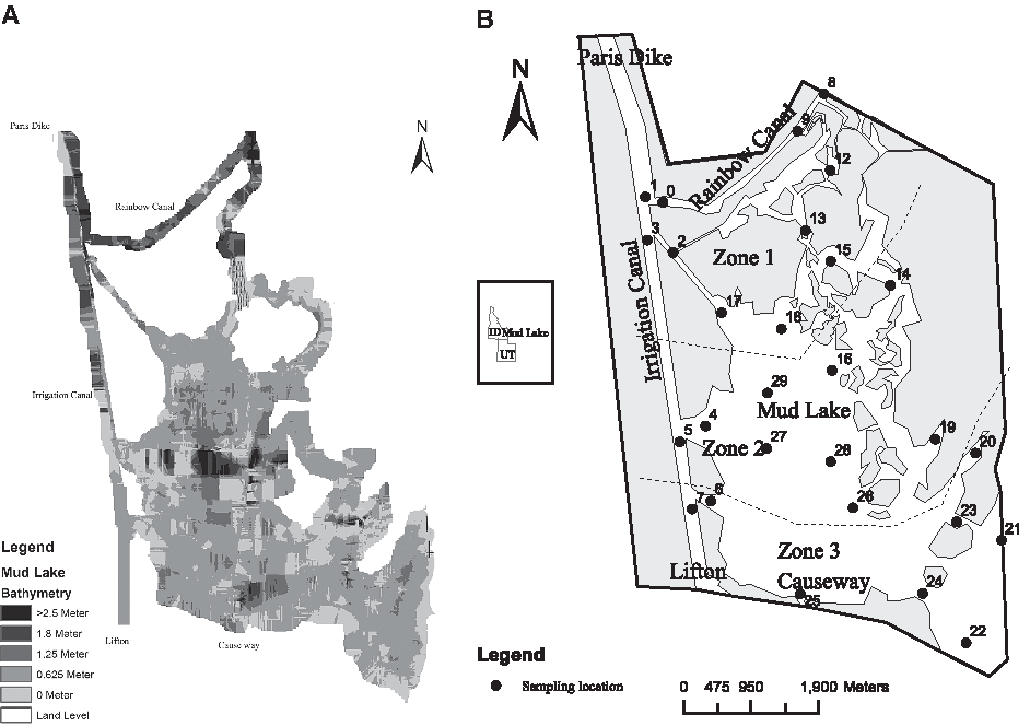
Mud Lake map as (A) bathymetry (B) sampling locations and zones (the dots mark the sample locations of change of hydraulics).

The current flow management strategy in Mud Lake is for downstream hydropower production and results in seasonal flow patterns that are annually variable because of differences in annual precipitation. The spatial distribution of suspended fine sediments in the light of complex hydrodynamics within Mud Lake, or any similar shallow impoundment, requires attention to spatial and temporal patterns in the data.

Objectives

We hypothesize and preliminary data collection suggested that the management of flow through Mud Lake produces the temporal and spatial patterns that would support MVRVM modeling to predict fine sediment concentrations and levels of other water quality constituents. We also introduce an experimental design that uses enough monitoring stations to confirm that we captured the dynamics of sediment in Mud Lake and that the MVRVM results will show how many locations are sufficient to build the model. Thus, the objectives of this research are to (1) evaluate the use of an MVRVM modeling approach and assess its efficacy in a complex hydraulic system with limited observations to model suspended fine sediment and water quality constituents, (2) expand the use of the MVRVM for the hydraulic and suspended fine sediment dynamics without the need of developing physics-based models, (3) verify that the collected data embody patterns that are required for effective use of the MVRVM, and (4) demonstrate that the data from the chosen locations are sufficient to capture the needed patterns resulting from operational time-based management of the lake.

In this article, we describe an experimental program for the collection of hydraulic data, turbidity, total suspended solids (TSS), and other water quality constituent data, and the production of hydrodynamic model output, as inputs to the MVRVM model. As mentioned briefly above, the characteristics of the data that will provide for the information needs of the MVRVM are that they possess consistent temporal and spatial patterns. The goal of this data collection program is to maximize the chance that the data collected will possess those patterns by considering the inherent seasonal hydrologic variability and the flow management scheme used.

It is possible to foresee several challenges in studying Mud Lake and similar systems.

1. Flow in Mud Lake is the driving force for patterns of all constituents in the Lake. However, the flow is controlled by a private third party who provided only flow estimates based on the daily average of recorded gate flow.

2. The magnitude and direction of the water velocity in the lake dictates the distribution of sediments. However, no historical velocity data inventory exists. Such data would allow identification of sediment distribution patterns and potential deposition patterns for different locations in the lake. Lack of knowledge of system hydrodynamics may contribute to filling some parts of the lake with sediment in the near future and limiting its usefulness as a refuge (BLWAMM, 2005).

3. In addition to fine sediment, the habitat for ducks and other waterfowls relies on the quality of water within Mud Lake and changes in operation can result in the loss of habitat (Bjornn, 1989).

To meet the challenges created by this complex natural system and achieve the objectives of our study, the following steps were taken.

1. Select monitoring locations: preliminary sampling revealed that the changes of hydraulic properties in the lake could be modeled by creating sampling locations that can track all the constituents' range of variability. To ensure that the MVRVM is provided with sufficient data to reproduce spatial and temporal patterns, thirty locations for monitoring and sampling were proposed as more than sufficient to track the suspended fine sediment circulating in Mud Lake.

2. Identify spatial and temporal patterns: spatial and temporal patterns were sought for suspended fine sediment water quality measures at the selected locations by monitoring over time at regular intervals at each location.

3. Examine flow scenarios: study of flow scenarios (e.g., spring and fall) combined with the transported suspended sediment will give a better understanding of the amount of fine sediment and water quality constituents in different locations in Mud Lake.

4. Create velocity inputs: flow scenarios are modeled to understand how the water flow is routed through Mud Lake. To do so, the MVRVM model requires flow velocities at each monitoring location; however, the large majority of velocity vector observations were below the detection limit of the instrumentation used. The collection for the 30 monitoring locations over 2 days showed that the velocity was measurable in only 7 locations even during high flow conditions. This necessitated the use of a mechanistic two-dimensional hydrodynamic model, CCHE2D (Zhang, 2005), to provide estimates of velocity vectors for each location to use as input for the MVRVM model.

Experimental design

The study aimed to collect and evaluate hydraulic, sediment-related, and water quality data to support the MVRVM modeling approach in the Mud Lake. The MVRVM approach has two requirements. First, the data must show subtle differences in patterns of sediment and other water quality constituents over time and space; and second, the data must be available in sufficient quantities that the MVRVM algorithm can discover those data that capture model-relevant information (relevance vectors), but exclude data that have little information content or are highly correlated with data that are retained by the MVRVM.

Sediment/water quality

The study of the fine sediment transport requires the study of the suspended load data. These data were obtained by weekly sampling during the ice-free periods of 2009 and 2010. TSS samples were collected at mid-depth using a Niskin type sampler (General Oceanic, Inc., Miami, FL), and TSS concentrations were measured at the Utah Water Research Laboratory following the procedure based on the US EPA Method 160.2 and Standard Methods 2540.D to determine the TSS concentration at all sampling locations. A Hydrolab Sonde series MS 5 (Hach Company, Loveland, CO) was used to measure the water quality constituent turbidity, pH, temperature, and dissolved oxygen (DO). The sensors were calibrated at the beginning and end of each field data collection trip. Statistical analysis was carried out using the R statistics package (Ihaka and Gentleman, 1996). For quality control purposes, we collected duplicate TSS samples for three random locations during every field trip. Analysis of the TSS duplicate samples showed that pooled coefficient of variation (standard deviation divided by the mean) was 0.5%, which compares well with the guidelines of EPA of 10% relative error being acceptable.

Velocity

Velocity measurements were made using an Acoustic Doppler profiler from the side of a boat at each of the monitoring stations. Collection of velocity observations was made difficult by the small velocity magnitude, usually below the detection limit of the instrumentation of 15 cm/s. Because of this, the velocity measurements were suspended early in the monitoring program and, as an alternative, the flow direction was observed indirectly in the field trips by noting the direction of the wake around on the current meter rod inserted in the flow stream, while the magnitude was estimated using the hydrodynamic model discussed above.

Results and Discussion

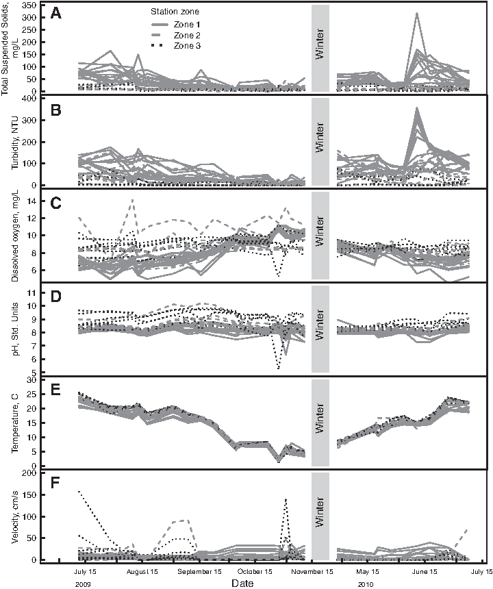
Flow data (Table 1) reveal that there are two main operating scenarios. The first is during the spring runoff season when the water flows from the Bear River via Rainbow Canal (Fig. 1) through the lake and into the adjacent Bear Lake. The second is during the late summer period when water is pumped from the Bear Lake back into Mud Lake to satisfy downstream irrigation requirements when the Bear River flow is not high enough to meet the irrigation demand (Fig. 2).

FIG. 2.

Box-whisker plots of collected observations in the 30 locations of Mud Lake during 2009–2010 as (A) DO, mg/L, (B) pH, standard units, (C) temperature, °C, (D) turbidity, NTU, (E) TSS, mg/L, and (F) velocity, cm/s. TSS, total suspended solids; DO, dissolved oxygen.

Table 1.

Operation Scenarios Used in Mud Lake as Inflows and Outflows in Mud Lake Measured in Rainbow Canal, Farmers Irrigation Canal, Causeway, and Lifton

	Flows location cfs
Day	Rainbow	Farmers	Causeway	Lifton
7/13/2009	800	986	0	360
7/30/2009	168	645	0	675
8/11/2009	144	424	0	360
8/14/2009	144	551	0	720
8/19/2009	207	571	0	345
9/2/2009	152	406	0	340
9/10/2009	140	328	0	340
11/2/2009	255	744	0	426
6/28/2010	857	1156	0	378
7/9/2010	485	708	0	1060
6/3/2009	919	5	983	0
9/19/2009	64	84	0	0
10/23/2009	220	5	131	0
10/29/2009	185	5	131	0
11/5/2009	256	194	0	0
11/12/2009	240	5	219	0
4/29/2010	200	5	219	0
5/19/2010	50	5	44	0
5/21/2010	135	5	44	0
5/28/2010	90	5	132	0
6/4/2010	160	5	132	0
6/11/2010	950	5	967	0
6/18/2010	2050	5	2050	0

The shaded cells represent summer 2009 operation scenario in the lake.

Assessment of water quality in Mud Lake

Dissolved oxygen

The minimum DO required for most aquatic life is 5–6 mg/L (DEQ, 2011). Fluctuations of DO levels can result from aquatic vegetation photosynthesis and respiration. Systems can lose DO due to decomposition of organic matter by bacteria and chemical reactions consuming oxygen. Low levels of DO can stress aquatic organisms and cause mortality (CEES, 2005). The levels of DO within Mud Lake were generally above the level for aquatic life; however, a small number of observations were recorded below the minimum in station 10 through 13 (Fig. 1) near where the Bear River flows into Mud Lake.

pH

Survival of aquatic organisms and health of an ecosystem require a specific range of pH [∼6.5–9.0 (DEQ, 2011)]. High pH can result from algae and aquatic vegetation using CO₂ for photosynthesis. Low pH, caused by respiration of the same organisms, can mobilize many toxic chemicals, particularly, heavy metals that become available for uptake by aquatic plants and animals, creating the potential for toxic conditions for aquatic life (CEES, 2005). Although the pH in Mud Lake was generally between 6.5 and 9, occasionally the pH fluctuated outside that range especially in the southeast corner of the lake, where the water is clear and plant density is high.

Water temperature

When temperature is outside the range, it can cause stress or death for aquatic organisms (CEES, 2005). Water temperature also influences the DO saturation in water that may strongly affect aquatic organisms. The Bull Trout standard for the state of Idaho is 9°C during spawning time (DEQ, 2011). The temperature range was spatially consistent throughout Mud Lake and varied temporally from near freezing to 25°C (Fig. 3).

FIG. 3.

Time series observations in the 30 locations of Mud Lake during 2009–2010 as (A) DO, mg/L, (B) pH, standard units, (C) temperature, °C, (D) turbidity, NTU, (E) TSS, mg/L, and (F) velocity, cm/s.

Turbidity and sediment

Increased sediment transport into water bodies has an impact on the quality of ecosystem required for the survival of inhabiting species (Schubel, 1977). Turbidity can reduce the light entering the water column and decrease photosynthesis from aquatic plants. Nutrients, particularly phosphorus, can adsorb onto sediment particles (Bjornn, 1989); thus, the spatial distribution of fine sediment is of great importance to determine the fate of nutrients (Schubel, 1977). Sediment can disrupt food production dynamics through decreased predator success with respect to prey survival (Moore, 1977; Simenstad, 1990; Coen, 1995). In the case of Mud Lake, the turbidity ranged from 0 NTU to 357 NTU [Idaho DEQ guidelines for turbidity state that the turbidity should be less than the background turbidity +50 NTU (DEQ, 2011)]. Figure 3 shows that from October, through the beginning of the runoff season, the turbidity is within the DEQ acceptable range, while during the rest of the year, the turbidity was often above 50 NTU. The patterns seen in the turbidity data are echoed in the TSS data.

Velocity vector magnitude

Velocity is the driving force responsible for determining the fate and transport of sediment through the lake. Because of their small magnitude, velocities were not as thoroughly quantified as the water quality constituents. The results from the hydrodynamic model (Fig. 3) showed that more than 90% of the velocity magnitudes are below the detection limit. The predicted velocity magnitudes were higher in the northern portion of the lake and decreased to near zero through the southern end.

Suitability of observations to the MVRVM

Field observations determined (Fig. 1) that Mud Lake could be divided into three zones (labeled Zone 1, Zone 2, and Zone 3 on Fig. 1), based on the location and on observed hydraulic and water quality similarities. Observations at some locations may be expected to be different than at other locations, due to ecological conditions observed during data collection, which might affect the modeling results. Some locations, especially in Zone 3, had significant aquatic vegetation and algae, which can affect the DO and pH observations and, since the observations reported here were taken during daylight, the DO and pH might be expected to be somewhat higher than the average over the day (Table 2).

Table 2.

Constituent Percentiles According to Zones in Mud Lakea

		Min	25 Percentile	50 Percentile	75 Percentile	Max
DO±0.2 mg/L	Zone 1	4.92	7.44	8.11	9.33	11.48
	Zone 2	4.48	6.81	7.88	9.35	11.19
	Zone 3	5.95	8.21	9.01	10.37	14.63
pH±0.2	Zone 1	6.35	7.98	8.12	8.26	8.95
	Zone 2	7.74	8.17	8.33	8.56	9.12
	Zone 3	5.22	8.32	8.62	9.07	10.18
Temperature±0.1 C	Zone 1	1.46	7.20	14.27	17.93	23.81
	Zone 2	1.41	7.91	14.88	18.82	25.01
	Zone 3	0.97	8.19	15.07	19.28	25.56
TSS±15% mg/L	Zone 1	0	14.67	27.67	52.00	170.67
	Zone 2	0	10.67	17.00	34.33	108.67
	Zone 3	0	3.33	6.00	10.67	100.00
Turbidity±3% NTU	Zone 1	0	19.38	49.75	94.55	357.30
	Zone 2	0	13.50	29.15	60.20	175.30
	Zone 3	0	0	2.95	14.48	78.40
Velocity magnitude 2%±1.5 cm/s	Zone 1	0	1.72	5.22	10.73	55.11
	Zone 2	0	0.07	0.40	3.14	91.64
	Zone 3	0	0	0.01	2.22	156.66

TSS, total suspended solids; DO, dissolved oxygen.

Zone 1 is characterized as a network of canals and provides the source for sediment into Mud Lake from the Bear River. Some parts of this zone are very shallow due to sediment deposition; during sampling, we observed that some channels have been dredged, to promote and distribute flow and sediment through all of Mud Lake (Bjornn, 1989). This zone is generally clear of vegetation in its water ways, but is vegetated between channels.

Zone 2 is near the center of Mud Lake with patchy vegetation; transition between turbid and clear water takes place in this zone. The vegetation is low-density rooted submerged vegetation (∼0.2 m height), which may affect the pH and DO observations.

Zone 3 is filled with rooted vegetation, often emergent, (>∼0.2 m height) at the majority of locations. The DO and pH increase significantly relative to Zones 1 and 2, likely due to the photosynthetic activity during the daytime sampling. Zone 3 is characterized by extremely low velocities, especially in the east, thus providing an opportunity for the fine sediment to settle, and leading to low TSS and turbidity.

Pattern type I (Figs. 2 and 3)

Temperature is characterized by consistent percentile ranges for observations at all the locations: the temperature pattern did not vary significantly between zones.

Pattern type II (Figs. 2 and 3)

pH and DO are characterized by change in the percentile range of observations across locations, especially in Zone 3, where there is an increase of vegetation and algae; this would be expected to increase the pH and DO observations relative to Zone 2, due to the presence of small amounts of vegetation in Zone 2 compared with Zone 3.

Pattern type III (Figs. 2 and 3 described by the turbidity, TSS, and velocity magnitude)

It is described by a variable range of change for percentiles in Zones 1 and 2, and then drop to near zero in Zone 3. The turbidity is related to the TSS; however, the accuracy of measuring turbidity is higher. TSS is heterogeneous and during collection of grab samples, we might capture clumps of sediment in either the sample or the smaller portion taken for filtering, which does not represent the whole water. These problems lead to errors in observing TSS as high as 10–20%.

The observations (Figs. 2 and 3) support the presence of patterns (the observations in every location with respect to time act in an arrangement of repeated features over the 2-year monitoring campaign) for all locations. The time series were used to represent the data during the ice-free periods for the three zones (Fig. 3). The general similarity among observations in each zone suggests that the MVRVM model, for which a subset of the observations is selected for model fitting, should have sufficient data for accurate representation of the variables at each sampling location.

Conclusion

The review of previous modeling efforts used for sediment transport emphasizes the conclusion that these models are less suitable to simulate the spatial sediment distribution because of the fine sediment nature of Mud Lake and low in-lake velocity. It was also demonstrated that the data collected embody patterns that can be useful for the use of the MVRVM, to capture the patterns resulting from time-based operation and management of the lake. The operation of the lake caused the presence of these patterns for the modeled constituents.

The observations show distinct patterns with respect to the flow conditions at each location and also reveal that some of the observations were outside the range designated by the Idaho Department of Environmental Quality that supports aquatic growth (DEQ, 2011). Even though we have large number of observations, experience has shown that they are insufficient to support the use of ANN or SVM models. We hypothesize that the data set is more than adequate for modeling using the MVRVM. As will be seen in the next article, the MVRVM shows promise in modeling systems with complex patterns not only in hydraulics, but also for modeling water quality constituents.

Footnotes

Acknowledgments

We would like to thank the Utah Water Research Laboratory for funding this research. We would also like to thank US Fish and Wildlife Service and PacifiCorp for their support during data collection. Special thanks to the Utah Water Research Laboratory team: Jim Millesan, Mark Winklaar, Chris Thomas, Shannon Clemens, Austin Jensen, Jeff Horsburgh, and Cody Allen.

References

ASCE Task Committee on Application of Artificial Neural Networks in Hydrology. 2000. Artificial neural networks in hydrology. I: Preliminary concepts. J. Hydrol. Eng., 5:115.

Assessment Data for Idaho, Medicine Lodge Watershed (ADIMLW). 2002. http://epadev.induscorp.com/epadevdb_tmdl_web/w305b_report_v2.hucp_huc=17040215&p_state=ID. 2009 March 31.

Babovic

2005. Data mining in hydrology. J. Hydrol. Process., 19:1511.

Babovic

, Abbott

1997. The evolution of equations from hydraulic data. Part I: Theory. J. Hydraul. Res., 35:397.

Bear Lake Watch Annual Membership Meeting (BLWAMM). 2005. www.bearlakewatch.com/membernotes/blwannmtg07.htm. 2009 March 31.

Bjornn

T.C.

1989. An evaluation of sediment and nutrient loading on fish and wildlife production at Bear Lake National Wildlife Refuge. Tech. Rep., 87:199.

Center of Earth and Earth Science (CEES). 2005. Use of long-term research for enhancing water quality in the Great Lakes Region. www.cees.iupui.edu/education/Workshops/Project_Seam/water_quality.htm. 2012 February .

Coen

L.D.

1995. A Review of the Potential Impacts of Mechanical Harvesting on Subtidal and Intertidal Shellfish Resources. Charleston, SC: South Carolina Department of Natural Resources, Marine Resources Research Institute.

Department of Environmental Quality Idaho (DEQ). 2011. Water Quality Standards. http://adminrules.idaho.gov/rules/2011/58/0102.pdf

10.

Dogan

, Ates

, Yılmaz

C.E.

, Eren

2008. Application of artificial neural networks to estimate wastewater treatment plant inlet BOD. Environ. Prog., 27:439.

11.

Dogan

, Sengörür

, Köklü

2009a. Modeling biological oxygen demand of the Melen River in Turkey using an artificial neural network technique. J. Environ. Manage., 90:1229.

12.

Dogan

, Tripathi

, Govindaraju

2007a. Application of relevance vector machine for sediment transport estimation. World Environmental and Water Resources Congress 2007, 1–10. 10.1061/40927(243)389.

13.

Dogan

, Tripathi

, Lyn

D.A.

, Govindaraju

R.S.

2009b. From flumes to rivers: Can sediment transport in natural alluvial channels be predicted from observations at the laboratory scale? Water Resour. Res., 45:W08433.

14.

Dogan

, Yuksel

, Kisi

2007b. Estimation of total sediment load concentration obtained by experimental study using artificial neural networks. Environ. Fluid Mech., 7:271.

15.

Ihaka

, Gentleman

1996. R: A language for data analysis and graphics. J. Comput. Graph. Stat., 5:299.

16.

Jain

S.K.

2001. Development of integrated sediment rating curves using ANNs. J. Hydrol. Eng., 127:30.

17.

Kisi

Ö.

, Yüksel

, Dogan

2008. Modelling daily suspended sediment of rivers in Turkey using several data driven techniques. Hydrol. Sci. J., 53:1270.

18.

Moore

P.G.

1977. Inorganic particulate suspensions in the sea and their effects on marine animals. Oceanogr. Mar. Biol. Ann. Rev., 15:225.

19.

Nagy

H.M.

, Watanabe

, Hirano

2002. Prediction of sediment load concentration in rivers using artificial neural network model. J. Hydraul. Eng., 6:588.

20.

Schubel

J.R.

1977. Sediment and the quality of the estuarine environment: some observations. Suffet

I.H.

Fate of Pollutants in the Air and Water Environments. Part 1. Mechanism of Interaction Between Environments and the Mathematical Modeling and the Physical Fate of Pollutants. New York: John Wiley and Sons, 399–424.

21.

Simenstad

C.A.

1990. Effects of Dredging on an Adromous Pacific Coast Fishes, Workshop Proceedings. Seattle, WA: University of Washington Sea Grant Program.

22.

Tipping

M.E.

2001. Sparse Bayesian learning and the relevance vector machine. J. Mach. Learn. Res., l:211.

23.

Vapnik

1995. The Nature of Statistical Learning Theory. New York: Springer-Verlag, Inc.

24.

, Liong

, Babovic

2004. EC-SVM approach for real-time hydrologic forecasting. J. Hydroinform., 6:209.

25.

Zhang

2005. CCHE2D Mesh Generator Users' Manual-Version 2.50. NCCHE Technical Report. NCCHE-TR-2005-01 January 2005.

Relevance Vector Machine Models of Suspended Fine Sediment Transport in a Shallow Lake—I: Data Collection

Abstract

Abstract

Introduction

Artificial neural networks

Support vector machines

Relevance vector machine

Materials and Methods

The study area and challenges

Objectives

Experimental design

Sediment/water quality

Velocity

Results and Discussion

Assessment of water quality in Mud Lake

Dissolved oxygen

pH

Water temperature

Turbidity and sediment

Velocity vector magnitude

Suitability of observations to the MVRVM

Pattern type I (Figs. 2 and 3)

Pattern type II (Figs. 2 and 3)

Pattern type III (Figs. 2 and 3 described by the turbidity, TSS, and velocity magnitude)

Conclusion

Footnotes

Acknowledgments

References