Influence of Soil Moisture on Soil Gas Vapor Concentration for Vapor Intrusion

Abstract

Mathematical models have been widely used in analyzing the effects of various environmental factors in the vapor intrusion process. Soil moisture content is one of the key factors determining the subsurface vapor concentration profile. This manuscript considers the effects of soil moisture profiles on the soil gas vapor concentration away from any surface capping by buildings or pavement. The “open field” soil gas vapor concentration profile is observed to be sensitive to the soil moisture distribution. The van Genuchten relations can be used for describing the soil moisture retention curve, and give results consistent with the results from a previous experimental study. Other modeling methods that account for soil moisture are evaluated. These modeling results are also compared with the measured subsurface concentration profiles in the U.S. EPA vapor intrusion database.

Introduction

In the 1970s and 1980s, residential indoor air quality became a focus of interest, in relation to both volatile organic compounds (VOCs) and radon. The assessment of extent and hazard posed by vapor intrusion of VOCs into buildings has received increasing attention in recent years (Murphy and Chan, 2011; Eklund et al., 2012; McHugh et al., 2012; Picone et al., 2012; Turczynowicz et al., 2012; Wang et al., 2012). With ∼500,000 contaminated sites in the United States presenting uncertain VOC vapor intrusion risk (Schuver, 2007), the assessment of risk from inhalation of these vapors has been a topic of recent discussion, field investigations (Fitzpatrick and Fitzgerald, 2002; Sanders and Hers, 2006; William et al., 2007), and modeling studies (Abreu and Johnson, 2005; DeVaull, 2007; Tillman and Weaver, 2007; Bozkurt et al., 2009; Pennell et al., 2009; Yao et al., 2011). In 2002, the U.S. EPA issued a draft guidance for vapor intrusion assessment (EPA, 2002), and new final guidance is imminent. Since the issuance of the draft guidance, many field data have been added to the U.S. EPA vapor intrusion database (EPA, 2012).

In the U.S. EPA document evaluating its vapor intrusion database (EPA, 2012), statistical tests have been used for examining attenuation factors (indoor air vapor concentration/subsurface vapor concentration) and for selecting various screening objectives. The subsurface measurements that are captured in this database include the subslab vapor concentration c_ss, the soil gas vapor concentration c_sg, and the vapor concentration c_gw calculated assuming equilibrium with groundwater contaminant concentration. The large variation in values of the ratio c_ss/c_gw as noted by EPA has been further examined in recent publications (Suuberg et al., 2011; Yao et al., 2012, 2013b, 2013c).

In our previous work (Shen et al., 2013a), a simplified analytical relation has been offered to describe the relationship between the subslab concentration c_ss and the soil gas concentration measured at some distance from a building of interest, c_sg. At steady state, the difference between these two vapor concentrations, if taken at the same depth below ground surface, arises from the slab capping effect. This diffusional blockage effect increases the concentration beneath the building slab relative to the open ground surface beneath it (Bozkurt et al., 2009; Shen et al., 2013a, 2013b). Therefore, it is important to consider the lateral distance of separation between any soil gas samples from any soil capping when evaluating the potential for risk, based upon those soil gas values. From our evaluation of the U.S. EPA database, it appeared that about 70% of the soil gas and groundwater samples were taken more than 15 m away from, but within 50 m of, the building they were assigned to. We assume here that such data points were far enough removed from any capping effect that they represent “open field” soil gas values. Considering such soil gas vapor concentration data points in the database, the number that are paired with corresponding groundwater vapor concentration data points is 182 for chlorinated hydrocarbons. The chlorinated hydrocarbon data are selected to avoid any complications in interpretation related to possible biodegradation, which can affect the petroleum-derived hydrocarbons. All of the selected data points are plotted in Fig. 1.

FIG. 1.

Soil gas vapor concentration as a function of groundwater vapor concentration assumed to be in equilibrium with groundwater, from the U.S. EPA vapor intrusion database.

The absolute values of both concentrations in Fig. 1 are seen to vary by more than six orders of magnitude. The dependency of c_sg on c_gw is not obvious. As is common in most vapor intrusion scenarios, the contaminant species dissolved in groundwater has been characterized as the main contaminant vapor source for all the data included in the database (EPA, 2012). However, Pearson's correlation coefficient R (Borradaile, 2003), widely used to assess the degree of association between a dependent response variable (the soil gas concentration) and an independent variable (the source concentration), is 0.14 confirming the weak correlation between even logarithmic values of c_gw and c_sg (EPA, 2012). In other words, there is no simple linear dependency observed between the source vapor concentration and the soil gas vapor concentration. The weak dependency can be the consequence of various specific site and sampling conditions, such as sampling locations (Abreu and Johnson, 2005), source concentration distribution (Yu et al., 2009), soil heterogeneity (Bozkurt et al., 2009), open ground surface capping effects (Shen et al., 2013a), transient effects, such as groundwater fluctuations (Picone et al., 2012), barometric changes (Garbesi and Sextro, 1989; McHugh et al., 2012), and so on. On the other hand, there is one major factor that often does not receive sufficient attention- that of soil moisture content. It is the influence of this factor that will receive attention in this manuscript.

Among the factors that characterize actual field conditions, soil moisture content is one of the most difficult to characterize, but among those with biggest effect on vapor concentration profiles (Sanders and Talimcioglu, 1997). The importance of soil moisture distribution has been pointed out in several field studies (Hers and Zapf-Gilje, 1998; Hers et al., 2000) and theoretical studies (McHugh and McAlary, 2009; EPA, 2012). In a review of vapor intrusion by the U.S. Department of the Navy (McAlary, et al., 2009), the need to better understand the soil texture and moisture effects on vapor intrusion was pointed out. Hers et al. (2003) mentioned that diffusive flux in the U.S. EPA (2004) implementation of the U.S. EPA Johnson and Ettinger model was significantly affected by a soil layer with high moisture content. While there is recognition of the importance of soil moisture content, there has been limited quantitative analysis related to its influence.

The vapor intrusion modeling studies related to soil moisture were mostly focused on transient effects (Sanders and Talimcioglu, 1997; Tillman and Weaver, 2007; Picone et al., 2012; Shen et al., 2012). A previous study (Shen et al., 2012) coupled transient soil water and gas flow processes with the vapor transport process. Such models are complicated to solve in two- or three-dimensions; therefore, previous work (Sanders and Talimcioglu, 1997; Tillman and Weaver, 2007; Picone et al., 2012; Shen et al., 2012) either simplified the scenarios into one-dimensional (1D) scenarios, or assumed quasi-equilibrium of either the flow or transport process. A full description of transient vapor transport processes must include the role of soil moisture, even in a hydrostatic state (Bear, 1988). Moreover, the soil moisture may affect open field soil gas profiles and subslab vapor concentration profiles differently.

Soil moisture distribution is characterized by three zones above the groundwater table—the surface soil layer, the vadose zone, and the capillary fringe. The capillary fringe is located immediately above the groundwater table, where liquid water is drawn into the soil pores by capillary forces. The capillary fringe extends upward from the groundwater table and the upper limit of this zone has an irregular shape (Bear, 1988). There may, however, sometimes also exist within the vadose zone a fully saturated “perched water” zone, with its own capillary zone, and of course there can be transient saturation of any of the layers. Here we do not consider this extra complexity.

Experimental and field measurements of soil moisture profiles are well established (Robinson et al., 2008; Vereecken et al., 2008). Empirical relations between pressure, saturation, and permeability (Burdine, 1953; Brooks and Corey, 1964; Jeppson, 1974; Mualem, 1976; Chen et al., 1999; van Genuchten, 1980) have been developed. One of the best known sets of descriptive equations, the van Genuchten relations, will be used in this manuscript to obtain a realistic soil moisture content profile in the hydrostatic state.

In this manuscript, we focus on comparing different methods for computing soil gas contaminant vapor concentration profiles for different soil types, which will allow evaluating the influence of different key variables, including moisture content, on these profiles. This will allow addressing the question of why there might at first appear to be a weak correlation between soil gas and source concentration values when comparing different vapor intrusion scenarios. Different modeling methods are compared, including those explicitly using the van Genuchten relations and others using a layered soil simplification. The results from a 1D vapor transport model, using the van Genuchten relations, will be shown to be consistent with results from a previous experimental study. It is noted that different assumptions of soil moisture content lead to very different results for the soil gas vapor concentration profiles. We finally compare the results from a vapor intrusion model assuming a uniform soil, with actual c_sg/c_gw values in the U.S. EPA database.

Modeling Methodology and Validation

A typical vapor intrusion modeling schematic is shown in Fig. 2. Consider first that a soil gas sampling point is located far from the building slab, as shown. Then a 1D model can be used to describe the soil gas vapor concentration profile, with boundary conditions c=c_gw at the groundwater surface and c=0 at the ground surface. If the soil between these boundaries, shown on the right of Fig. 2, were uniform in transport properties, then the resulting contaminant gas profile would of course be linear. The governing equation and boundary conditions are shown in Table 1. It should be noted that if the effective soil gas diffusivity is a function of height (z), then the concentration profile cannot be linear. A finite element code, COMSOL, is used in solving the equations, when we take into account such variability in soil properties. The contaminant is assumed to be uniformly distributed in the groundwater beneath the whole modeling domain. Considerations of the lateral separation of source from building structure have been included in previous research (Murphy and Chan, 2011; Yao et al., 2013a). The vapor concentration immediately above the groundwater table is calculated assuming Henry's law.

FIG. 2.

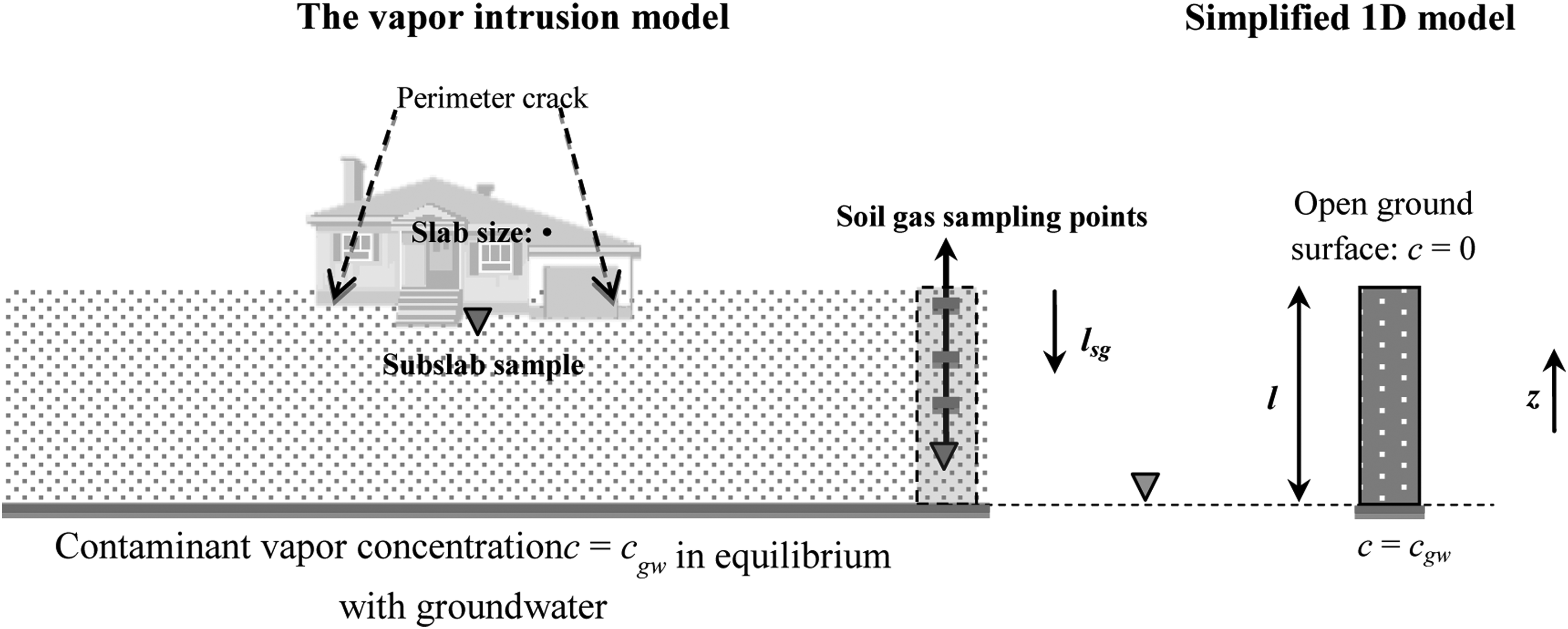
Typical vapor intrusion modeling scenario and simplified one-dimensional modeling scenario for soil gas.

Table 1.

Equations and Boundary Conditions

Governing equation
Contaminant vapor transport	\documentclass{aastex}\usepackage{amsbsy}\usepackage{amsfonts}\usepackage{amssymb}\usepackage{bm}\usepackage{mathrsfs}\usepackage{pifont}\usepackage{stmaryrd}\usepackage{textcomp}\usepackage{portland, xspace}\usepackage{amsmath, amsxtra}\pagestyle{empty}\DeclareMathSizes{10}{9}{7}{6}\begin{document} $$ \frac { \partial } { \partial z } \left( D^ { eff } \frac { \partial } { \partial z } c \right) = 0 \quad\quad\quad\quad\quad\quad\quad\quad\quad\ \ \ ( 1 )$$ \end{document}
Boundary conditions
Contaminant source	c=c_gw
Open field	c=0
Constitutive equations
van Genuchten relations (van Genuchten, 1980)	\documentclass{aastex}\usepackage{amsbsy}\usepackage{amsfonts}\usepackage{amssymb}\usepackage{bm}\usepackage{mathrsfs}\usepackage{pifont}\usepackage{stmaryrd}\usepackage{textcomp}\usepackage{portland, xspace}\usepackage{amsmath, amsxtra}\pagestyle{empty}\DeclareMathSizes{10}{9}{7}{6}\begin{document} $$ \frac { \theta_w - \theta_r } { \theta_t - \theta_r } = \left[ 1 + ( \alpha^{} H_c ) ^ { 1 / ( 1 - M^ {} ) } \right] ^ { - M^ {*} } \ \quad\quad \, ( 2 )$$ \end{document}
	\documentclass{aastex}\usepackage{amsbsy}\usepackage{amsfonts}\usepackage{amssymb}\usepackage{bm}\usepackage{mathrsfs}\usepackage{pifont}\usepackage{stmaryrd}\usepackage{textcomp}\usepackage{portland, xspace}\usepackage{amsmath, amsxtra}\pagestyle{empty}\DeclareMathSizes{10}{9}{7}{6}\begin{document} $$\theta_g = \theta_t - \theta_w \quad\quad\quad\quad\quad\quad\quad\quad\quad ( 3 )$$ \end{document}
Relative permeability for water flow	\documentclass{aastex}\usepackage{amsbsy}\usepackage{amsfonts}\usepackage{amssymb}\usepackage{bm}\usepackage{mathrsfs}\usepackage{pifont}\usepackage{stmaryrd}\usepackage{textcomp}\usepackage{portland, xspace}\usepackage{amsmath, amsxtra}\pagestyle{empty}\DeclareMathSizes{10}{9}{7}{6}\begin{document} $$k_{r , w} = Se_w^{1 / 2} \left[ 1 - \left( 1 - Se_w^{1 / M^{}} \right) M^{} \right] ^2 \ ( 4 )$$ \end{document}
Relative permeability for soil gas flow	\documentclass{aastex}\usepackage{amsbsy}\usepackage{amsfonts}\usepackage{amssymb}\usepackage{bm}\usepackage{mathrsfs}\usepackage{pifont}\usepackage{stmaryrd}\usepackage{textcomp}\usepackage{portland, xspace}\usepackage{amsmath, amsxtra}\pagestyle{empty}\DeclareMathSizes{10}{9}{7}{6}\begin{document} $$k_{r , g} = ( 1 - Se_w ) ^{1 / 3} \left( 1 - Se_w^{1 / M^{}} \right) ^{2M^{}} \ \ \ \quad( 5 )$$ \end{document}
Henry's law	\documentclass{aastex}\usepackage{amsbsy}\usepackage{amsfonts}\usepackage{amssymb}\usepackage{bm}\usepackage{mathrsfs}\usepackage{pifont}\usepackage{stmaryrd}\usepackage{textcomp}\usepackage{portland, xspace}\usepackage{amsmath, amsxtra}\pagestyle{empty}\DeclareMathSizes{10}{9}{7}{6}\begin{document} $$c_{gw} = K_H c_{GW} \ \quad\quad\quad\quad\quad\quad\quad\quad\quad\quad \ \ ( 6 )$$ \end{document}
Effective in-soil diffusivity using Millington–Quirk equation (Millington and Quirk, 1961)	\documentclass{aastex}\usepackage{amsbsy}\usepackage{amsfonts}\usepackage{amssymb}\usepackage{bm}\usepackage{mathrsfs}\usepackage{pifont}\usepackage{stmaryrd}\usepackage{textcomp}\usepackage{portland, xspace}\usepackage{amsmath, amsxtra}\pagestyle{empty}\DeclareMathSizes{10}{9}{7}{6}\begin{document} $$D^ { eff } = D_g \frac { \theta_g^ { 10 / 3 } } { \theta_t^2 } + \frac { D_w } { K_H } \frac { \theta_w^ { 10 / 3 } } { \theta_t^2 } \quad\quad\quad\quad\quad\quad \ ( 7 )$$ \end{document}
Effective in-soil diffusivity using Moldrup equation (Kristensen et al., 2010)	\documentclass{aastex}\usepackage{amsbsy}\usepackage{amsfonts}\usepackage{amssymb}\usepackage{bm}\usepackage{mathrsfs}\usepackage{pifont}\usepackage{stmaryrd}\usepackage{textcomp}\usepackage{portland, xspace}\usepackage{amsmath, amsxtra}\pagestyle{empty}\DeclareMathSizes{10}{9}{7}{6}\begin{document} $$D^ { eff } = D_g \frac { \theta_g^ { 2.5 } } { \theta_t } + \frac { D_w } { K_H } \frac { \theta_w^ { 2.5 } } { \theta_t } \ \quad\quad\quad\quad\quad\quad \ \ \ ( 8 )$$ \end{document}
Effective in-soil diffusivity using accounting for dispersion (Atteia and Hohener, 2010)	\documentclass{aastex}\usepackage{amsbsy}\usepackage{amsfonts}\usepackage{amssymb}\usepackage{bm}\usepackage{mathrsfs}\usepackage{pifont}\usepackage{stmaryrd}\usepackage{textcomp}\usepackage{portland, xspace}\usepackage{amsmath, amsxtra}\pagestyle{empty}\DeclareMathSizes{10}{9}{7}{6}\begin{document} $$D^ { eff } = D_g \frac { \theta_g^ { 10 / 3 } } { \theta_t^2 } + \frac { D_w } { K_H } \frac { \theta_w^ { 10 / 3 } } { \theta_t^2 } + \xi_z \ u_ { GW } \ \frac { k_ { r , w } } { K_H } \ \quad( 9 )$$ \end{document}

See Nomenclature for definitions of mathematical variables.

The van Genuchten relations [Eqs. (2) and (3)] basically use two main parameters, α* and M*, for defining the soil moisture retention curve. The parameter α* scales the capillary pressure head or the elevation above the groundwater table (in steady state), and M* determines the curvature of the retention curve. The van Genuchten parameters are commonly obtained from laboratory tests for field soil samples.

The soil moisture content is related to the capillary pressure head which is sometimes called the “suction” or “matrix suction”: \documentclass{aastex}\usepackage{amsbsy}\usepackage{amsfonts}\usepackage{amssymb}\usepackage{bm}\usepackage{mathrsfs}\usepackage{pifont}\usepackage{stmaryrd}\usepackage{textcomp}\usepackage{portland, xspace}\usepackage{amsmath, amsxtra}\pagestyle{empty}\DeclareMathSizes{10}{9}{7}{6}\begin{document} \begin{align*}H_c = \frac { p_c } { \rho_w g } = \frac { p_g - p_w } { \rho_w g } \tag { 10 } \end{align*} \end{document}

keeping in mind that this property is also related to water surface tension. Setting the groundwater table as the datum, at steady state when the gas phase pressure gradient is relatively small as compared to water pressure gradient, then \documentclass{aastex}\usepackage{amsbsy}\usepackage{amsfonts}\usepackage{amssymb}\usepackage{bm}\usepackage{mathrsfs}\usepackage{pifont}\usepackage{stmaryrd}\usepackage{textcomp}\usepackage{portland, xspace}\usepackage{amsmath, amsxtra}\pagestyle{empty}\DeclareMathSizes{10}{9}{7}{6}\begin{document} \begin{align*}H_c = - \frac { p_w } { \rho_w g } = z \tag {11} \end{align*} \end{document}

where z is the pressure head in terms of elevation above the datum, and which is then used as the z-axis with zero point reference at the groundwater level. It is this value of H_c that is used in Equation (2) to obtain the moisture content distribution when gas pressure head is ignored.

The height of the capillary fringe is here represented by the capillary pressure head at the inflection point of the retention curve when soil moisture content is plotted as a function of log(H_c) (Dexter and Bird, 2001): \documentclass{aastex}\usepackage{amsbsy}\usepackage{amsfonts}\usepackage{amssymb}\usepackage{bm}\usepackage{mathrsfs}\usepackage{pifont}\usepackage{stmaryrd}\usepackage{textcomp}\usepackage{portland, xspace}\usepackage{amsmath, amsxtra}\pagestyle{empty}\DeclareMathSizes{10}{9}{7}{6}\begin{document} \begin{align*}H_ { c , \inf } = \frac { 1 } { \alpha^* } \left( \frac { 1 } { M^* } \right) ^ { { 1 - M } ^* } \tag { 12 } \end{align*} \end{document}

Soil gas or moisture advection in transient processes, such as with atmospheric pressure change (Picone et al., 2012), groundwater level fluctuation (Picone et al., 2012), and rainfall (Tillman and Weaver, 2007; Shen et al., 2012), have been considered in previous work and are ignored here.

An experimental study (McCarthy and Johnson, 1993) of soil moisture distribution in sandy soil is considered as a basis for a 1D modeling scenario. The reported measured soil moisture content profile, shown in Fig. 3a was first curve fit by us, using the Levenberg–Marquardt algorithm, giving the van Genuchten parameters: α*=5.31/m, M*=0.834, θ_r=0.0142, θ_t=0.351. These parameters are close to those obtained by others for the same data set (Atteia and Hohener, 2010). In the McCarthy and Johnson experimental study, trichloroethylene (TCE) was selected to be the contaminant vapor and this compound was introduced into simulated groundwater at the bottom of the experimental soil column. From this simulated groundwater source, the evaporation of the TCE took place into the soil. The simulated groundwater velocity was 0.1 m/day. The steady state vapor concentration profile for this experimental situation may be calculated using the equations in Table 1, and the results are shown in Fig. 3.

FIG. 3.

Measurements of soil moisture profile and its curve fit using the van Genuchten relations (a) and calculated soil gas contaminant vapor profile (b) showing effects of different dispersivity assumptions.

Dispersion was also taken into account when modeling this experimental column study. When considering mechanical dispersion (often simply termed dispersion) (Gelhar et al., 1992) induced by groundwater flow, the most relevant process in the contaminant vapor transport through soils is in the transverse vertical direction (here, the z-direction) (Klenk and Grathwohl, 2002; Olsson and Grathwohl, 2007). For groundwater flow in the unsaturated zone, Atteia and Hohener (2010) suggested modifying the Millington–Quirk equation as shown in Equation (9). The third term of Equation (9) accounts for the dispersion contribution to diffusion through the capillary zone, resulting from the groundwater flow below that zone.

The soil moisture content is observed to be an important factor in determining soil permeability, diffusivity, and dispersivity. It can be seen how steep the contaminant gradient is through the high moisture content capillary fringe, as compared to the relatively drier soil above. The predicted values of TCE concentration using the Millington–Quirk approximation for soil vapor diffusivity agree well with the experimentally measured values, but are sensitive to the assumed value of dispersivity, as seen in Fig. 3b. Another commonly used equation for describing the diffusion through the capillary fringe, the Moldrup equation (Kristensen et al., 2010), gives values quite similar to those from the Millington–Quirk equation, at zero dispersion. Obviously adding a similar dispersion consideration into the Moldrup equation can likewise improve its fit to the data.

The ratio of c_sg/c_gw decreased about two orders of magnitude within the shaded area, that is, in the capillary fringe, which is about 0.2 m thick above the groundwater table. This thickness was calculated by using Equation (12). Hence, the critical role of the capillary zone in reducing soil vapor concentration from its value at the source is affirmed. This model, taking into account the predicted structure of the capillary fringe, is now applied to considering how contaminant vapor concentration profiles in other soils can be influenced by similar processes.

Results and Discussion

The above cited laboratory study was conducted using sandy soil. The capillary fringe thickness for other soil types can be calculated using appropriate van Genuchten parameters. In the U.S. EPA Johnson and Ettinger model, the van Genuchten parameters for 12 kinds of soil type (SCS soils) are given in that reference (EPA, 2004). The approximate capillary zone thickness for each soil type is also given, though these were calculated using a different method (EPA, 2004), which is not used here. The comparison of the capillary fringe thicknesses obtained using Equation (12) and the values in the U.S. EPA Johnson and Ettinger model are shown in Table 2. The soil moisture retention curves for sand, sandy loam and clay are shown in the left panels of Fig. 4 as examples. It is worth noting that sand is a more likely aquifer medium than is clay. The left hand panels compare the predictions for the true capillary zone profiles (the smooth curves) to the predictions of a pseudo-capillary zone thickness, from the EPA method (EPA, 2004). Note that in this latter method, the capillary zone is characterized by a single moisture content, and the soil above it by another single moisture value.

FIG. 4.

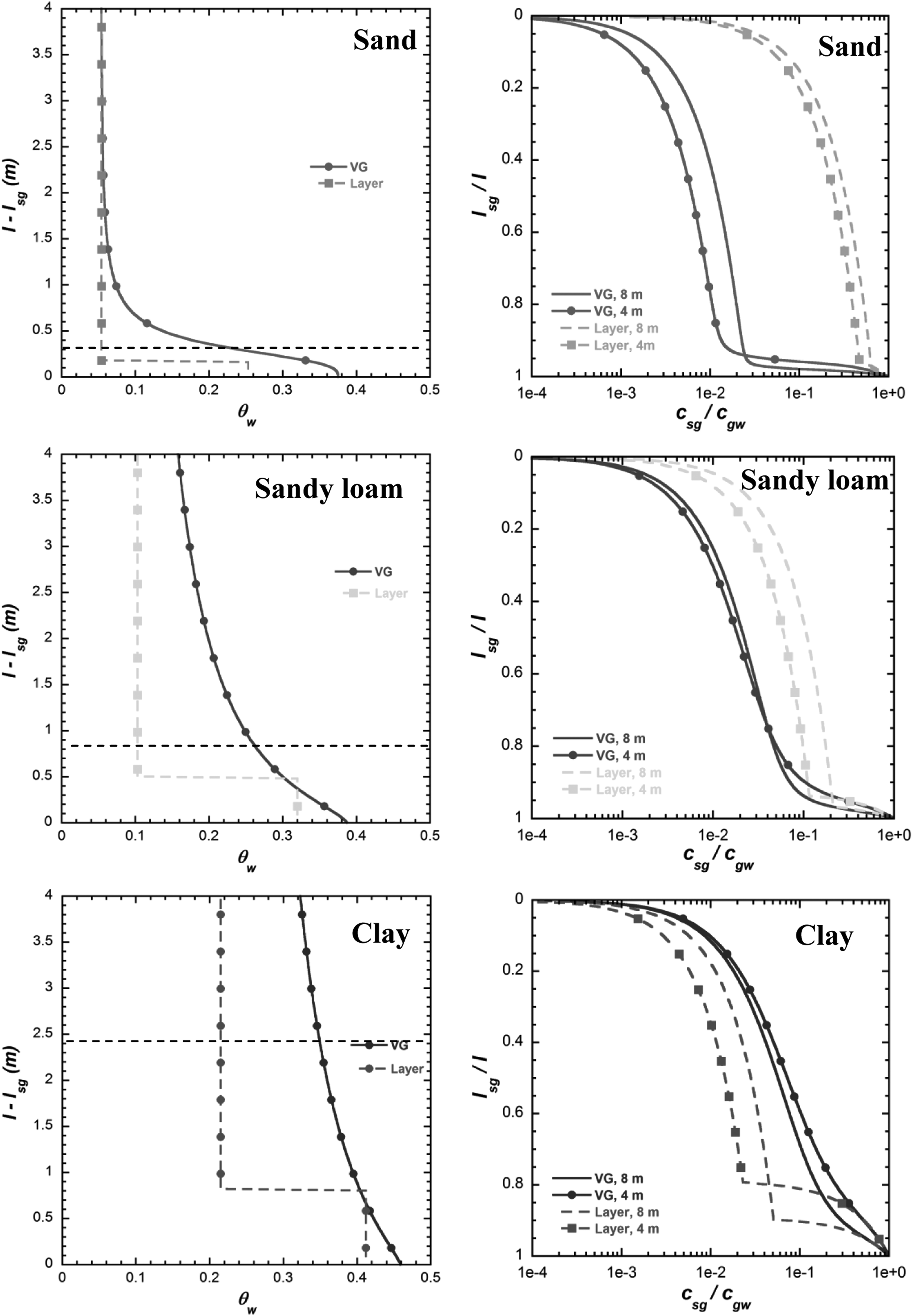
Left: Soil moisture profiles calculated using both van Genuchten (VG) relations and U.S. EPA Johnson and Ettinger model built-in values (assuming a layered soil). Right: Calculated soil gas concentration profiles plotted as a function of depth below ground surface (bgs) divided by total soil column depth. Horizontal dashed lines are located at the top of capillary fringe calculated using Equation (12).

Table 2.

Capillary Fringe Thickness

SCS soil name	Capillary fringe thickness using Equation (4) (m)	Capillary fringe thickness in U.S. EPA Johnson and Ettinger model [derived in Eqs. (8)–(10) in EPA (2004)] (m)
Clay loam	1.5	0.47
Silty clay	1.8	1.92
Silty clay loam	2.41	1.34
Sandy clay	1.28	0.3
Loam	1.95	0.38
Sandy clay loam	1.35	0.26
Clay	2.4	0.82
Silt loam	3.44	0.68
Sandy loam	0.84	0.25
Silt	2.61	1.63
Loamy sand	0.47	0.19
Sand	0.32	0.17

Soil types are ranked by intrinsic permeability from smallest value to largest.

It should be noted that the assigned SCS soil names are only qualitative descriptors of the properties of many different types of soil. A single set of van Genuchten parameters or capillary rise thicknesses may not represent the possible variability in quantitative parameters. In fact, data on soil properties (Carsel and Parrish, 1988) show that most of the different soil types overlap each other to some extent. Despite the fact that “sand” is expected to have a lower capillary rise than “clay,” “sand” itself consists of very coarse or very fine materials which would have very different van Genuchten parameter values.

After calculating the soil moisture distributions, numerical solutions for the vapor concentration profiles were obtained and are shown on the right hand panels of Fig. 4. Here for simulation purposes the conditions were selected to represent tetrachloroethylene (PCE) vapor transport, though the results are not particularly sensitive to that choice, since they are shown as nondimensional concentrations relative to source concentration (predicted from Henry's law). The soil was taken to be isothermal at 10°C. The total height of the soil column from the groundwater table to the open surface was taken as either 4 or 8 m. The vertical axes are the soil gas sampling depths (bgs) divided by the total soil column length.

The moisture content curve for sand, obtained from the van Genuchten relations, breaks very abruptly, as its van Genuchten parameter M* is the smallest of all soil types. This, in turn, results in the sharpest decline in the vapor concentration profile through the capillary fringe, as seen in the solid curves in the right panel. The abrupt break in the contaminant concentration profile is associated with the very strong influence of moisture content on vapor diffusivity through the capillary zone. It can be seen that the detailed prediction of the moisture profile is somewhat mirrored in the simple “layered soil” prediction; both give fairly thin capillary zones as compared to those for other soil types. However, the predicted influence of the capillary zone on contaminant vapor profiles is vastly different for the two different capillary zone models. The layered soil model does not predict the nearly two order of magnitude decrease of contaminant concentration across the capillary zone. This can clearly have major implications for accurate prediction of vapor intrusion potential.

In contrast to the above, clay soil shows the least distinct capillary zone, as calculated using the van Genuchten method, and shown in the left panel of Fig. 4. Consequently there is not a very drastic change in vapor diffusivity across the capillary zone. Thus, in this case, the contaminant vapor concentration profile is the smoothest, through the capillary zone. The soil vapor concentration profiles using van Genuchten relations are different than that using a layered soil model with the same source depth, but not to the same degree as in the case of sand.

In all cases, the two-layer approximation from the U.S. EPA spreadsheet shows a different predicted capillary zone thickness than that calculated using the inflection point method of Equation (12). This can significantly impact prediction of vapor profiles, as is clearly visible in Fig. 4. With sandy soils, orders of magnitude uncertainty in vapor concentration may be involved, whereas in other cases, only roughly an order of magnitude difference is noted.

Thus, one of the significant reasons to define a capillary fringe thickness is to enable proper calculation of the effective soil vapor diffusivity. Vapor intrusion models often assume uniform soil properties, including averaged soil moisture content and thus, employ uniform diffusivity values for the soil. As vapor diffusion is the primary process of interest in vapor intrusion, two different methods to obtain the vapor diffusivity are compared here.

Considering a uniform soil example, the U.S. EPA Johnson and Ettinger model treats the capillary zone and unsaturated soil as two separate, but uniform, layers, as shown in the left panels of Fig. 4. In the U.S. EPA Johnson and Ettinger model, a total effective diffusivity (Hers et al., 2002) is defined using a series resistance model, involving the wet and dry soil layers: \documentclass{aastex}\usepackage{amsbsy}\usepackage{amsfonts}\usepackage{amssymb}\usepackage{bm}\usepackage{mathrsfs}\usepackage{pifont}\usepackage{stmaryrd}\usepackage{textcomp}\usepackage{portland, xspace}\usepackage{amsmath, amsxtra}\pagestyle{empty}\DeclareMathSizes{10}{9}{7}{6}\begin{document} \begin{align*}D_ { t } ^ { eff } = \frac { l } { \frac { l_1 } { D_1^ { eff } } + \frac { l - l_1 } { D_0^ { eff } } } \tag { 13 } \end{align*} \end{document}

An alternative method involves assuming a realistic water retention curve, either from direct measurement of the soil moisture content at different vertical locations, or by relating the soil to the already-defined soil type with associated van Genuchten parameters as was done above. Then, the total effective diffusivity is calculable only by integration: \documentclass{aastex}\usepackage{amsbsy}\usepackage{amsfonts}\usepackage{amssymb}\usepackage{bm}\usepackage{mathrsfs}\usepackage{pifont}\usepackage{stmaryrd}\usepackage{textcomp}\usepackage{portland, xspace}\usepackage{amsmath, amsxtra}\pagestyle{empty}\DeclareMathSizes{10}{9}{7}{6}\begin{document} \begin{align*}D_ { t } ^ { eff } = \frac { l } { \int \limits_0^1 \frac { dz } { D^ { eff } } } \tag { 14 } \end{align*} \end{document}

Equations (13) and (14) can be used for calculating the vapor flow rate across a horizontal area in a 1D model. However, if a total effective diffusivity is used to obtain the subsurface vapor concentration profile, the soil moisture profile is assumed to be constant (linear) and the details of profile in the capillary fringe are ignored. Thus, c_sg/c_gw linearly increases with the sampling depth (bgs), as a simple consequence of the Fickian diffusion law. There is also a linear relation between c_sg and c_gw when sampling depth is fixed (Fischer and Uchrin, 1996). This linear vapor concentration profile is shown in Fig. 5b. Note that while the rate of contaminant transport depends upon the actual value of diffusivity, the concentration profile cannot, which is why there is only a single curve shown for the constant diffusivity case.

FIG. 5.

Ratios of soil gas vapor concentration to groundwater vapor concentration in U.S. EPA vapor intrusion database. (a) Concentration ratios are plotted with respect to absolute elevation above groundwater table. (b) Concentration ratios are plotted with respect to relative sampling depth bgs.

The above result needs to be compared with the actual field data, shown as the data points in Fig. 5. The data from Fig. 1 for which there were vertical location information provided, are plotted in Fig. 5a and b as nondimensional soil gas vapor concentrations obtained by dividing the soil gas concentration by the corresponding groundwater vapor concentrations (c_sg/c_gw).

In Fig. 5a, the concentration ratio is plotted as a function of the absolute elevation of the soil gas sampling point above the groundwater table. It can be seen that a large fraction of the soil gas samples were taken within 4 m above the groundwater table. A variation of five orders of magnitude in c_sg/c_gw (10⁻⁴–10) can be seen within this range of elevation. It is apparent from these data that they reflect very different vapor phase diffusional resistances in a zone quite near the water table (and thus, near the capillary zone).

In Fig. 5b, the same data points are replotted as a function of their sampling depth (l_sg) below the open ground surface (bgs), rather than the elevation above the groundwater table as in Fig. 5a. Plotted in this manner, the data may be compared with the types of concentration profiles predicted above. Most of the data points fall several orders of magnitude below the earlier discussed solid line obtained assuming D^eff=constant, showing that a linear relation obtained in this way will generally over-predict actual soil gas vapor concentration. That is, the concentration ratio predicted from the constant effective diffusivity curve generally occurs at a higher than actually observed ratio of l_sg/l, meaning that higher concentrations are predicted higher in the soil column than are typically observed. The calculation results, using the soil moisture profiles based upon the van Genuchten relations, are also shown in Fig. 5b. The results from these models begin to show better agreement when comparing to the field measured concentration ratios, in that lower values of (c_sg/c_gw) are predicted for any value of l_sg/l, as compared with the constant diffusivity case. In fact, the curves for this realistic set of soils begin to capture many of the actual database values, though there are still some that are quite a bit lower for reasons that remain unclear.

It can also be seen from Fig. 5b is that the dashed and dotted curves become somewhat linear in the upper part of the vadose zone when l_sg<< l; that is, c_sg/c_gw increases almost linearly with l_sg/l near the open field surface. This is true for all 12 kinds of soils listed in Table 2, for soil columns either 4 or 8 m in height (results for all soils not shown). This is easily understood in terms of the low moisture content of the upper portions of the soil column, such that the local effective diffusivity is no longer a strong function of height.

The above results indicate the importance of characterizing the details of soil moisture profile and thus, the effective diffusivity in the soil. The above comparison is intended to show the difference that the choice of calculation method for soil diffusivity might lead to, particularly when making an assumption of single effective diffusivity, based on the series resistance of two soil layers.

It is clear that measurements of soil gas contaminant vapor concentration will very much depend on the depth of soil gas sampling. If it is not known what the influence and location of the capillary fringe is, such data may be very difficult to interpret. The available field data on soil gas concentrations obtained at “higher” and “lower” locations, relative to the open ground surface are plotted in Fig. 6. In Fig. 6a, the data are chosen to be those with l_sg/l<0.5, meaning that they are obtained relatively closer to the surface, whereas in Fig. 6b, they are chosen to be those for l_sg/l≥0.5, meaning closer to the source. This cutoff depth ratio was arbitrarily chosen here. We know that the data involve various soil types that have different capillary fringe thicknesses (Table 2). We are fairly certain that many of the data in Fig. 6a are above the capillary fringe. Once again, the great variability in near surface soil gas contaminant concentrations may be seen at just around the source concentration of 10⁻³ μg/m³. This means that the difference in resistances below these depths already spread the soil gas concentrations over several orders of magnitude. The same may be seen when one goes deeper into the soil. In both Fig. 6a and b, the soil gas vapor concentrations both appear to increase with increasing groundwater concentration, though the soil gas concentrations in Fig. 6a extend three orders of magnitude lower than those in Fig. 6b. If all the data in Fig. 6a and b were to be plotted together, there would again be no clear trend of soil gas concentration with c_gw. This helps explain the apparently low correlation coefficient of the data in Fig. 1. That is to say, when limited data sets are examined, the expected concentration profile trends might be expected. On the other hand, when all data, for many soil types involving many different types of resistances are examined together, the underlying trends may no longer be nearly as visible.

FIG. 6.

Soil gas vapor concentration versus the groundwater vapor concentration in the U.S. EPA vapor intrusion database. (a) The data point is chosen to be that the paired soil gas sampling depth bgs compared to the paired groundwater depth bgs is <0.5. (b) The data point is chosen to be that the paired soil gas sampling depth bgs compared to the paired groundwater depth bgs is ≥0.5.

Conclusion

This paper illustrates the importance of the soil moisture content in determining soil gas vapor concentration profiles. While there is no standard method currently in use for describing the soil moisture profile in vapor intrusion modeling, different methods can result in very different predictions of soil gas concentration profiles. As soil gas sampling is an integral part of field investigations, attention should be paid to the effect of soil moisture content profiles in interpreting such data. These observations may have relevance in explaining some of the apparent discrepancy between field data and EPA Johnson and Ettinger model predictions, in particular, on why filed measurements of soil gas concentrations are generally lower than model results.

The above analysis also shows the importance of groundwater source sampling locations at a given site. Groundwater taken from within the capillary fringe may well offer a very different picture than the deeper groundwater, due to the large concentration gradient in the capillary fringe. The inclusion of soil moisture measurements in the field study was presented by Pennell et al. (2013). The usage of a conceptual model, including consideration of soil moisture variation for the specific site was evaluated.

Footnotes

Acknowledgment

This project was supported by Grant P42ES013660 from the National Institute of Environmental Health Sciences.

Author Disclosure Statement

No competing financial interests exist.

References

Abreu

L.D.V.

, Johnson

P.C.

2005. Effect of vapor source-building separation and building construction on soil vapor intrusion as studied with a three-dimensional numerical model. Environ. Sci. Technol., 39:4550.

Atteia

, Hohener

2010. Semianalytical model predicting transfer of volatile pollutants from groundwater to the soil surface. Environ. Sci. Technol., 44:6228.

Bear

1988. Dynamics of Fluids in Porous Media. Mineola, NY: Courier Dover Publications, Inc.

Borradaile

G.J.

2003. Statistics of Earth Science Data: Their Distribution in Time, Space and Orientation. Berlin, Germany: Springer.

Bozkurt

, Pennell

K.G.

, Suuberg

E.M.

2009. Simulation of the vapor intrusion process for nonhomogeneous soils using a three dimensional numerical model. Ground Water Monit. Remed., 29:92.

Brooks

R.H.

, Corey

A.T.

1964. Hydraulic Properties of Porous Media. Hydrology Papers. Fort Collins, CO: Colorado State University, 24.

Burdine

1953. Relative permeability calculations from pore-size distribution data. Petr. Trans. Am. Inst. Mining Metall. Eng., 198:71.

Carsel

R.F.

, Parrish

R.S.

1988. Developing joint probability distributions of soil water retention characteristics. Water Resour. Res., 24:755.

Chen

, Hopmans

, Grismer

1999. Parameter estimation of two-fluid capillary pressure-saturation and permeability functions. Adv. Water Resour., 22:479.

10.

DeVaull

G.E.

2007. Indoor vapor intrusion with oxygen-limited biodegradation for a subsurface gasoline source. Environ. Sci. Technol., 41:3241.

11.

Dexter

, Bird

2001. Methods for predicting the optimum and the range of soil water contents for tillage based on the water retention curve. Soil Till. Res., 57:203.

12.

Eklund

, Beckley

, Yates

, McHugh

T.E.

2012. Overview of state approaches to vapor intrusion. Remediat. J., 22:7.

13.

EPA. 2002. OSWER Draft Guidance for Evaluating the Vapor Intrusion to Indoor Air Pathway from Groundwater and Soils (Subsurface Vapor Intrusion Guidance)EPA530-D-02-004http://www.epa.gov/osw/hazard/correctiveaction/eis/vapor/complete.pdf.

14.

EPA. 2004. User's Guide for Ealuating Subsurface Vapor Intrusion Into BuildingsEPA Contract Number: 68-W-02-33http://www.epa.gov/oswer/riskassessment/airmodel/pdf/2004_0222_3phase_users_guide.pdf.

15.

EPA. 2012. EPA's Vapor Intrusion Database: Evaluation and Characterization of Attenuation Factors for Chlorinated Volatile Organic Compounds and Residential BuildingsEPA 530-R-10-002http://www.epa.gov/oswer/vaporintrusion/documents/OSWER_2010_Database_Report_03-16-2012_Final.pdf.

16.

Fischer

, Uchrin

C.G.

1996. Laboratory simulation of VOC entry into residence basements from soil gas. Environ. Sci. Technol., 30:2598.

17.

Fitzpatrick

N.A

, Fitzgerald

J.J.

2002. An evaluation of vapor intrusion into buildings through a study of field data. Soil Sediment. Contam., 11:603.

18.

Garbesi

, Sextro

R.G.

1989. Modeling and field evidence of pressure-driven entry of soil gas into a house through permeable below-grade walls. Environ. Sci. Technol., 23:1481.

19.

Gelhar

L.W.

, Welty

, Rehfeldt

K.R.

1992. A critical review of data on field-scale dispersion in aquifers. Water Resour. Res., 28:1955.

20.

Hers

, Zapf-Gilje

1998. Canadian consortium research project: Field validation of soil gas transport to indoor air pathway. In Proceedings of the 1998 Petroleum Hydrocarbon and Organic Chemicals in Ground Water Conference. Houston, TX: API/NGWA, 251.

21.

Hers

, Atwater

, Li

, Zapf-Gilje

2000. Evaluation of vadose zone biodegradation of BTX vapours. J. Contam. Hydrol., 46:233.

22.

Hers

, Zapf-Gilje

, Evans

, Li

2002. Comparison, validation, and use of models for predicting indoor air quality from soil and groundwater contamination. Soil Sediment Contam., 11:491.

23.

Hers

, Zapf-Gilje

, Johnson

P.C

, Li

. 2003. Evaluation of the Johnson and Ettinger model for prediction of indoor air quality. Ground Water Monit. Remed., 23:119.

24.

Jeppson

1974. Axisymmetric infiltration in soils, II. Summary of infiltration characteristics related to problem specifications. J. Hydrol., 23:191.

25.

Klenk

, Grathwohl

2002. Transverse vertical dispersion in groundwater and the capillary fringe. J. Contam. Hydrol., 58:111.

26.

Kristensen

A.H.

, Thorbjørn

, Jensen

M.P.

, Pedersen

, Moldrup

2010. Gas-phase diffusivity and tortuosity of structured soils. J. Contam. Hydrol., 115:26.

27.

McAlary

, Ettinger

, Johnson

, Eklund

, Hayes

, Chadwick

D.B.

, Rivera-Duarte

2009. Review of Best Practices, Knowledge and Data Gaps, and Research Opportunities for the U.S. Department of Navy Vapor Intrusion Focus Areas. Technical Report, 1982 San Diego, CA: SSC Pacific.

28.

McCarthy

K.A.

, Johnson

R.L.

1993. Transport of volatile organic compounds across the capillary fringe. Water Resour. Res., 29:1675.

29.

McHugh

T.E.

, McAlary

2009. Important physical processes for vapor intrusion: A literature review. In Proceedings of AWMA Vapor Intrusion Conference, San Diego, CA.

30.

McHugh

T.E.

, Beckley

, Bailey

, Gorder

, Dettenmaier

, Rivera-Duarte

, Brock

, MacGregor

I.C.

2012. Evaluation of vapor intrusion using controlled building pressure. Environ. Sci. Technol., 46:4792.

31.

Millington

, Quirk

. 1961. Permeability of porous solids. Trans. Faraday Soc., 57:1200.

32.

Mualem

1976. A new model for predicting the hydraulic conductivity of unsaturated porous media. Water Resour. Res., 12:513.

33.

Murphy

B.L.

, Chan

W.R.

2011. A multi-compartment mass transfer model applied to building vapor intrusion. Atmos. Environ., 45:6650.

34.

Olsson

, Grathwohl

2007. Transverse dispersion of non-reactive tracers in porous media: A new nonlinear relationship to predict dispersion coefficients. J. Contam. Hydrol., 92:149.

35.

Pennell

K.G.

, Bozkurt

, Suuberg

E.M.

2009. Development and application of a three-dimensional finite element vapor intrusion model. J. Air Waste Manage., 59:447.

36.

Pennell

K.G.

, Scammell

M.K.

, McClean

M.D.

, Ames

, Weldon

, Friguglietti

, Suuberg

E.M.

, Shen

, Indeglia

P.A.

, Heiger-Bernays

W.J.

2013. Sewer gas: An indoor air source of PCE to consider during vapor intrusion investigations. Ground Water Monit. Remed., 33:119.

37.

Picone

, Valstar

, van Gaans

, Grotenhuis

, Rijnaarts

2012. Sensitivity analysis on parameters and processes affecting vapor intrusion risk. Environ. Toxicol. Chem., 2012:31.

38.

Robinson

, Campbell

, Hopmans

, Hornbuckle

, Jones

, Knight

, Ogden

, Selker

, Wendroth

2008. Soil moisture measurement for ecological and hydrological watershed-scale observatories: A review. Vadose Zone J., 7:358.

39.

Sanders

P.F.

, Hers

2006. Vapor intrusion in homes over gasoline contaminated ground water in Stafford, New Jersey. Ground Water Monit. Remed., 26:63.

40.

Sanders

P.F.

, Talimcioglu

N.M.

1997. Soil‐to‐indoor air exposure models for volatile organic compounds: The effect of soil moisture. Environ. Toxicol. Chem., 16:2597.

41.

Schuver

2007. Vapor Intrusion: risks and challenges. EM, 2007 Feb. 6.

42.

Shen

, Pennell

K.G.

, Suuberg

E.M.

2012. A numerical investigation of vapor intrusion—The dynamic response of contaminant vapors to rainfall events. Sci. Total Environ., 437:110.

43.

Shen

, Pennell

K.G.

, Suuberg

E.M.

2013a. Analytical modeling of the subsurface volatile organic vapor concentration in vapor intrusion. Chemosphere, 15:1444.

44.

Shen

, Pennell

K.G.

, Suuberg

E.M.

2013b. Modeling quantification of the influence of soil moisture on subslab vapor concentration. Environ. Sci. Processes Impacts, 15:1444.

45.

Suuberg

, Yao

, Shen

, Bozkurt

, Pennell

2011. Modeling vapor intrusion processes and evaluating risks using subslab data. Environ. Health Biomed., 15:115.

46.

Tillman

F.D.

, Weaver

J.W.

2007. Temporal moisture content variability beneath and external to a building and the potential effects on vapor intrusion risk assessment. Sci. Total Environ., 379:1.

47.

Turczynowicz

, Pisaniello

, Williamson

2012. Health risk assessment and vapor intrusion: A review and Australian perspective. Hum. Ecol. Risk Assess., 18:984.

48.

van Genuchten

M.T.

1980. A closed-form equation for predicting the hydraulic conductivity of unsaturated soils. Soil Sci. Soc. Am. J., 44:892.

49.

Vereecken

, Huisman

, Bogena

, Vanderborght

, Vrugt

, Hopmans

2008. On the value of soil moisture measurements in vadose zone hydrology: A review. Water Resour. Res, 44:W00D06.

50.

Wang

, Unger

A.J.A.

, Parker

B.L.

2012. Simulating an exclusion zone for vapour intrusion of TCE from groundwater into indoor air. J. Contam. Hydrol., 140–141, 124.

51.

William

, Liu

, Rigby

M.C.

, Brenner

2007. Time-variable simulation of soil vapor intrusion into a building with a combined crawl space and basement. Environ. Sci. Technol., 41:4993.

52.

Yao

, Shen

, Pennell

K.G.

, Suuberg

E.M.

2011. Comparison of the Johnson-Ettinger vapor intrusion screening model predictions with full three-dimensional model results. Environ. Sci. Technol., 45:2227.

53.

Yao

, Shen

, Pennell

K.G.

, Suuberg

E.M.

2012. Examination of the influence of environmental factors in contaminant vapor concentration attenuation factor with U.S. EPA's vapor intrusion database. Environ. Sci. Technol., 47:906.

54.

Yao

, Shen

, Pennell

K.G.

, Suuberg

E.M.

2013a. Estimation of contaminant subslab concentration in vapor intrusion including lateral source-building separation. Vadose Zone J., 12. 10.2136/vzj2012.0157.

55.

Yao

, Shen

, Pennell

K.G.

, Suuberg

E.M.

2013b. Examination of the U.S. EPA's Vapor Intrusion Database based on models. Environ. Sci. Technol., 47:1425.

56.

Yao

, Shen

, Pennell

K.G.

, Suuberg

E.M.

2013c. A review of vapor intrusion models. Environ. Sci. Technol., 47:2457.

57.

, Unger

A.J.A.

, Parker

2009. Simulating the fate and transport of TCE from groundwater to indoor air. J. Contam. Hydrol., 107:140.