Computational Study of Surface Signature of Anthropogenic CO 2 at a Potential Carbon Sequestration Site,San Juan Basin

Abstract

Injection of anthropogenic carbon dioxide into geologic formations is a technology that can be deployed in the relatively short term in order to avoid potential harm to the environment caused by excess CO₂ in the atmosphere. Success of sequestering CO₂ in underground reservoirs is strongly dependent on the prevention of leakage back into the atmosphere and the ability to mitigate should significant leakage occur. Both detection of leakage and reliable risk mitigation plans require a robust monitoring system. The space and time span of CO₂ sequestration projects is large, which results in trade-offs between cost and robustness of monitoring. In order to make a cost-effective decision without compromising monitoring effectiveness, knowledge of CO₂ transport in the vadose zone and seepage mechanisms into the atmosphere is essential. This study focuses on the simulations of hypothetical CO₂ leakage into the ∼100 m thick vadose zone at an actual site in the San Juan Basin, the United States. Hypothetical leaks were assumed to occur through abandoned wellbores whose integrity had been compromised below the water table. Results show that, at the leak rates analyzed, CO₂ did not express itself at the wellhead for extended periods due to the extremely thick vadose zone. It was also seen that even after decades of simulated leakage, point measurements of CO₂ flux into the atmosphere may not reach levels distinguishable from the background. The regional seepage pattern, however, is both measurable and distinguishable. This finding can be used for designing cost-effective and robust near-surface monitoring networks and algorithms.

Introduction

Geologic sequestration of carbon is one of the solutions in the portfolio that is used to mitigate the effects on the environment due to anthropogenic greenhouse gas emissions. Main geologic storage candidates under consideration are deep saline aquifers, depleted oil and gas reservoirs, and unminable coal seams. Among these, deep saline aquifers are the least penetrated ones, and they constitute the larger portion of the storage potential (Kolenkovic et al., 2013).

Depleted oil and gas reservoirs are next in the list of targets for carbon sequestration due to their suitable reservoir permeability and proven capability to contain buoyant fluids for geologic time scales (Gentzis, 2000), as well as their potential to offset costs by enhanced production. Targeted storage reservoirs have a caprock that traps the injected CO₂ through various mechanisms. For some cases, the caprock itself can sorb the CO₂ diffusing into it, resulting in a self-blocking mechanism (Busch et al., 2008).

Ideally, storage reservoirs and formations are selected so that containment targets for CO₂ are met. However, many wells have often been drilled through oil and gas reservoirs. Considering that oil and gas extraction has a history of more than a century, one can easily see that some of the wells are older, were permitted under past regulations, and may carry a risk of allowing or enhancing fluid leakage from the target reservoirs (Patroni, 2007). Furthermore, many abandoned wells may have been “lost” due to inadequate record keeping. Such possibilities should be assessed in objective risk mitigation plans and by environmental impact analyses, because they may cause leaks (Koornneef et al., 2012).

A well that was drilled for oil or gas extraction is potentially subject to several hazards during its lifetime and after abandonment. These can be briefly listed as follows:

During the drilling: casing wear due to high rotating hours (Sun et al., 2012) or pressure and temperature cycles (van der Kuip et al., 2011), cracks within the wellbore cement, or target formation (Brown and Ferg, 2005).

After drilling: cement shrinkage followed by crack formation and/or cement-rock debonding (van der Kuip et al., 2011), exposure to formation fluids (Le Guen et al., 2009), and crack formation due to geologic movements (Mainguy et al., 2007).

When CO₂ is introduced into depleted oil and gas reservoirs, the hazards mentioned earlier will contribute to the risks of leakage. These risks include a leakage along or around the wellbore into the formations above the targeted one. In addition, the presence of CO₂ in the reservoir can pose further problems due to the effect that CO₂-saturated brine has on traditional Portland cement (Barlet-Gouédard et al., 2007; Kutchko et al., 2007). It should be noted that current research suggests that it is not likely that CO₂ will create a permeable pathway for any great distance along a wellbore, but that it could alter an existing pathway through the cement (Huerta et al., 2011) or at the cement-rock interface (Carey et al., 2007).

Given the original depth and the path it needs to travel, it is unlikely that significant rates of CO₂ leakage into the environment would occur (van der Kuip et al., 2011). As a testimony to this fact, during the 30 year history of CO₂ injection for enhanced oil recovery in Alberta, Canada, failures never reached a point to threaten the public safety (Bachu and Watson 2009). Recently, another claim of CO₂ leakage from the Weyburn sequestration project in Saskatchewan, Canada, was confirmed to be a false alarm, confirming the safety and reliability of the application (Romanak and Sherk, 2013). Another factor that may reduce the surface flux of a potential leak is the possible partitioning of the leaking fluid through the leaky portions of several wells, resulting in out-of-reservoir underground containment and a very diffuse signature near the surface (Pawar et al., 2009). Therefore, it is a challenge to monitor leakage events from the surface.

Due to the vulnerabilities explained so far and the attenuation of leakage as it travels underground, a sequestration project should verify its promise for long-term containment. This involves the monitoring of the movement of the injected CO₂ (Mathieson et al., 2009) and the detection of any potential leakages (Yang et al., 2011; Sun et al., 2013). In this regard, to study the behavior of leaking CO₂ in the vadose zone and to check the performance of the available detection technologies, controlled CO₂-release experiments (Lewicki et al., 2007; Strazisar et al., 2009; Spangler et al., 2010) and computational simulations (Oldenburg and Unger, 2004; Ogretim et al., 2009) have been performed.

Computer simulations are easier and cheaper to do, whereas on-site experimentation with actual equipment is costly, which increases the already existing financial burden related to carbon sequestration. Therefore, optimized and refined methods are necessary to meet the monitoring targets without increasing the costs significantly. Use of site-specific identifiers (Helium or tracer gases, etc.) (Annunziatellis et al., 2008) or perfluorocarbon tracers, soil gas monitoring (Strazisar et al., 2009), and distinguishing the temporal and/or spatial behavior of natural and artificial CO₂ fluxes (Lewicki et al., 2005; Pan et al., 2010; Romanak et al., 2013) are among the methods that have been investigated for this purpose.

After deep saline aquifers and depleted oil and gas reservoirs, unminable coal seams form a third option for geologic sequestration of carbon. It is known that coal seams often contain significant amounts of methane, which is generated during the formation of coal (Harpalani and Chen, 1995). With the improvement of available technology, such as hydraulic fracturing (Rahman et al., 2007; Wang, 2009), coal bed methane has become a significant source of fuel both in the United States and around the world (Economides et al., 2012) in the past few decades. In addition, when exposed to CO₂, coal desorbs methane as it adsorbs the carbon dioxide. Coal can sorb approximately 15 times as much CO₂ as methane by volume (Mazumder and Wolf, 2008). So, enhanced coal bed methane (ECBM) production is a method of carbon storage that has both environmental and economic benefits.

Several field tests have been held around the world to determine the feasibility of this idea, including at the Allison unit (Ozdemir, 2009; Shi and Durucan, 2010) and the Pump Canyon site in the San Juan Basin, which is a part of the U.S. Department of Energy's Southwest Regional Carbon Sequestration Partnership (Wilson et al., 2012). It should be noted that the wells which are going to be drilled for this purpose are going to be made from CO₂-resistant cement, and so will not suffer from the risks related to CO₂ exposure. However, there are other risks as discussed earlier, which still affect these new wells.

Storage in the San Juan Basin coal seam

For a detailed description of this basin and its geology, see the papers by Marroquin and Hart (2004) and Shuck et al. (1996). ECBM production with CO₂ involves the dewatering of the reservoir and the subsequent methane production in order to open up the pore space and increase injectivity. Although with the injection of CO₂, swelling of coal (Korre et al., 2007; Siriwardane et al., 2012) and the subsequent decrease in injectivity were observed in both the Allison unit and Pump Canyon field tests, long-term consistency in the injection rate may result in excess stress, which can induce microfractures that will improve near-wellbore permeability and, therefore, injectivity (Harpalani and Mitra, 2010).

The San Juan Basin is the top producer of coal bed methane in the world (Marroquin and Hart, 2004). Natural fractures present in the reservoir result in a high system-level permeability (Hart, 2006; Clarkson et al., 2010), and they make it possible to produce this field at economically attractive rates. The upper methane-containing coal seam is at 800–850 m (2600–2800 ft) below the surface (Shuck et al., 1996). With the contraction of the coal matrix due to the desorption of methane, the system permeability of coal generally increases during years of production (Mavor and Vaughn, 1998; Palmer, 2009; Pillalamarry et al., 2011). Using various well drilling and completion technologies, the gas recovery efficiency has increased to such levels that this single basin is a major source of natural gas in the United States (Palmer, 2010). Given its current status and the experiments already performed, the San Juan Basin is a potential target for CO₂ ECBM activity in the long term.

The present study uses computer simulations to investigate how a leak at the Pump Canyon site in the San Juan Basin (Fig. 1) would express itself in the near surface, and how readily it would be seen by monitoring devices at the surface. Similar studies have been performed at locations with shallow vadose zones and flat terrains (Lewicki et al., 2005; Lewicki et al., 2007; Yang et al., 2011). The unique aspect of the site used in this study is that the vadose zone spans approximately 140 m (Fig. 2), and the terrain is very irregular (Fig. 1). Although in the current study a CBM site is used, the risks pertaining to carbon sequestration under deep vadose zones are valid for the other geologic storage options explained earlier.

FIG. 1.

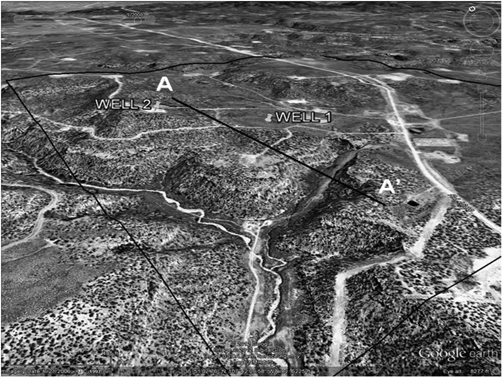
Overview of the simulated area from Google Earth and the locations of the wells where leakage was simulated.

FIG. 2.

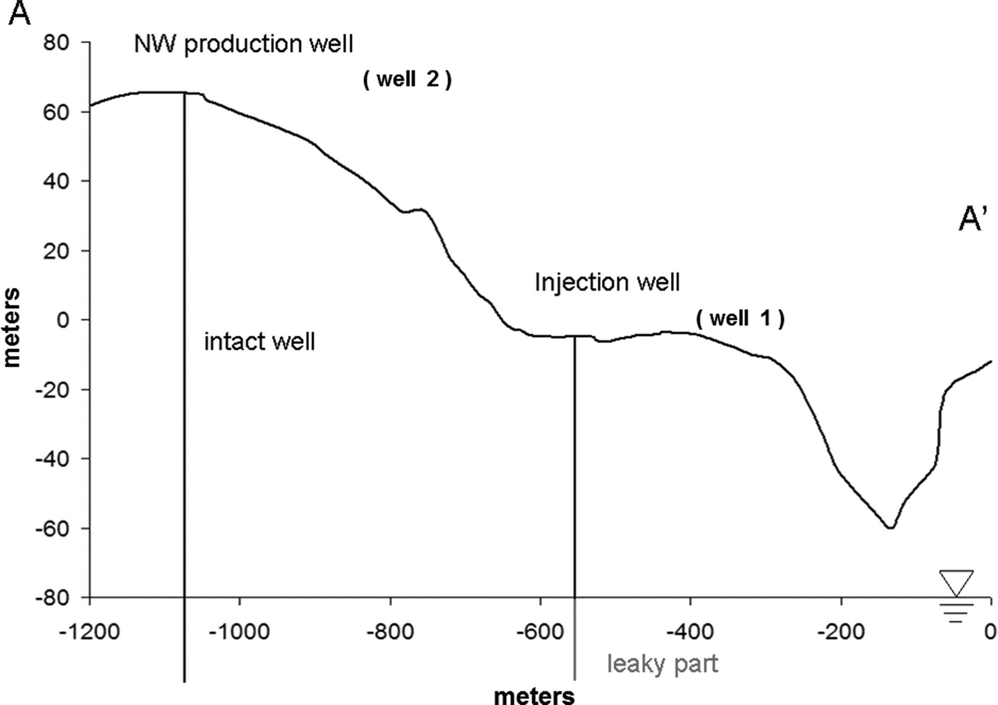
Sketch of the vadose zone along the A–A′ transect in Fig. 1 showing leakage from injection well.

In this study, we consider the possible leakage of CO₂ along a wellbore from a deep source and into the vadose zone. The development of the plume in the vadose zone from such a leak was simulated for two different wells shown in Fig. 1. The surface seepage flux distribution was analyzed to extract some lessons for the improvement of surface monitoring techniques that are applicable at other locations having thick vadose zones.

Methods

In the event of an accidental release of CO₂ from its reservoir, the path back to the atmosphere goes through several formations. Along this path, CO₂ can disperse into these formations, and it can dissolve in the resident fluids. On its way toward the surface, the CO₂ plume can branch into several paths due to heterogeneity of the medium. In the vadose zone, the vertical migration of the leaking CO₂ plume is impeded due to its negative buoyancy here. As a result of all these factors, only a small fraction of the original CO₂ leak may reach the surface. Therefore, a leakage of concern, even if it stays as a single branch throughout its path, may reveal a faint signature at or near the surface. To simulate such a case, three arbitrary leakage rates (10⁻⁴, 10⁻³, and 10⁻² kg/s) were simulated as point sources at the top of the water table at each well. Assuming 5 Mt of annual CO₂ emission from a mid-sized power plant, these leakage rates would correspond to leakage rates that are “less than critical,” “critical,” and “more than critical” levels, respectively, according to the criterion given in the IPCC Special Report on Carbon Capture and Storage (Metz et al., 2005).

Simulations were performed with the TOUGH2 code (Pruess et al., 1999) and its EOS7CA module (Oldenburg and Unger, 2003). Handling of the surface and manipulation of the computational grid accordingly was done by using an in-house preprocessor, INCONCEPT. The preprocessor uses the real topological data to automatically decide which grid cells fall in the computational domain and which do not. Subsequently, it assigns the cells at the surface as boundary cells.

For the simulations, permeability of the topsoil (first 0.5 m from the surface) was experimentally found using samples of the site. The remaining information was determined through observations of the site stratigraphy and the available publications on it (Mavor and Vaughn, 1998; Shi and Durucan, 2010; Wilson et al., 2012). The general stratigraphy of the actual site is such that thin layers of shale are present between thick layers of sandstone. To model this layered structure, a single anisotropic rock type was assumed in which horizontal permeability was 100 times higher than the vertical permeability. Further details on the underground layers and the corresponding functions for capillary pressure and relative permeability are given in Table 1.

Table 1.

Porous Medium Properties Used in the Computational Study

Property	Topsoil	Rock	Well
Porosity	0.2	0.05	0.5
Vertical permeability	1.0×10⁻¹³ m²	1.0×10⁻¹⁵ m²	1.0×10⁻¹² m²
Relative permeability^a
λ	0.7	0.4	0.9
S_lr	0.17	0.12	0.05
S_ls	1.0	1.0	1.0
S_gr	0.1	0.05	0.15
Capillary pressure^b
λ	0.7	0.4	0.9
S_lr	0.15	0.10	0.05
1/P₀ (Pa⁻¹)	2.04×10⁻⁴	1.48×10⁻³	2.04×10⁻³
P_max	5×10⁵	5×10⁵	5×10⁵
S_ls	1.0	1.0	1.0

van Genuchten function for relative permeability: for gases: \documentclass{aastex}\usepackage{amsbsy}\usepackage{amsfonts}\usepackage{amssymb}\usepackage{bm}\usepackage{mathrsfs}\usepackage{pifont}\usepackage{stmaryrd}\usepackage{textcomp}\usepackage{portland, xspace}\usepackage{amsmath, amsxtra}\pagestyle{empty}\DeclareMathSizes{10}{9}{7}{6}\begin{document} $$k_{rg} = \left( 1 - \hat{S} \right) ^2 \left( 1 - \hat{S}^2 \right)$$ \end{document} for liquids: \documentclass{aastex}\usepackage{amsbsy}\usepackage{amsfonts}\usepackage{amssymb}\usepackage{bm}\usepackage{mathrsfs}\usepackage{pifont}\usepackage{stmaryrd}\usepackage{textcomp}\usepackage{portland, xspace}\usepackage{amsmath, amsxtra}\pagestyle{empty}\DeclareMathSizes{10}{9}{7}{6}\begin{document} $$k_{rt} = \sqrt{S^*} \left\{ 1 - \left( 1 - \left[ S^* \right] ^{1 / \lambda} \right) ^ \lambda \right\} ^2$$ \end{document}

van Genuchten function for capillary pressure: \documentclass{aastex}\usepackage{amsbsy}\usepackage{amsfonts}\usepackage{amssymb}\usepackage{bm}\usepackage{mathrsfs}\usepackage{pifont}\usepackage{stmaryrd}\usepackage{textcomp}\usepackage{portland, xspace}\usepackage{amsmath, amsxtra}\pagestyle{empty}\DeclareMathSizes{10}{9}{7}{6}\begin{document} $$P_{\rm cap} = - P_0 \left( [ S^* ] ^{ - 1 / \lambda} - 1 \right) ^{1 - \lambda}$$ \end{document} where \documentclass{aastex}\usepackage{amsbsy}\usepackage{amsfonts}\usepackage{amssymb}\usepackage{bm}\usepackage{mathrsfs}\usepackage{pifont}\usepackage{stmaryrd}\usepackage{textcomp}\usepackage{portland, xspace}\usepackage{amsmath, amsxtra}\pagestyle{empty}\DeclareMathSizes{10}{9}{7}{6}\begin{document} $$- P_{ \max} \le P_{\rm cap} \le 0$$ \end{document} \documentclass{aastex}\usepackage{amsbsy}\usepackage{amsfonts}\usepackage{amssymb}\usepackage{bm}\usepackage{mathrsfs}\usepackage{pifont}\usepackage{stmaryrd}\usepackage{textcomp}\usepackage{portland, xspace}\usepackage{amsmath, amsxtra}\pagestyle{empty}\DeclareMathSizes{10}{9}{7}{6}\begin{document} $$S^* = ( S_l - S_{lr} ) / ( S_{ls} - S_{lr} )$$ \end{document} \documentclass{aastex}\usepackage{amsbsy}\usepackage{amsfonts}\usepackage{amssymb}\usepackage{bm}\usepackage{mathrsfs}\usepackage{pifont}\usepackage{stmaryrd}\usepackage{textcomp}\usepackage{portland, xspace}\usepackage{amsmath, amsxtra}\pagestyle{empty}\DeclareMathSizes{10}{9}{7}{6}\begin{document} $$\hat{S} = ( S_l - S_{lr} ) / ( 1 - S_{lr} - {S_{gr}} )$$ \end{document}

The computational domain included two wells, as shown in Fig. 1. Well 1 is an injection well at the center and well 2 is a production well to the northwest. It was assumed that both of these wells were abandoned after a future CO₂ ECBM production activity. Simulations were performed within the vadose zone to see the fate and surface signature of the CO₂ leaking through these wells.

For each simulation, only one well was assumed to be leaky. A rough sketch of the cross-section of the vadose zone along the A–A′ transect of Fig. 1 is shown in Fig. 2 for the case of leakage from well 1. Note that although this figure is two dimensional for illustration purposes, the simulations were three dimensional and were based on actual topography.

The computational domain included around 30,000 cells of various sizes, concentrating around the leaking well. For each case, the coordinates were adjusted so that the leaking well was located at the origin of the coordinate axes. Leakage simulations were preceded by an initialization run to achieve gravity-capillary equilibrium. During the initialization run, and later during the CO₂ injection runs, atmospheric conditions were assumed static; hence, temperature and pressure fluctuations at the surface were not accounted for. Then, the CO₂ was injected at a constant rate at the groundwater table directly under the well head for a simulated time of 40 years. For the boundary conditions on the computational domain, fixed-pressure and constant-zero-CO₂ concentration were used. The resultant seepage patterns were compared with two criteria: (1) a background value of 7.6 g/(m²·day), typical of arid biomes (Cable et al., 2011) similar to those found at the San Juan Basin site; (2) the minimum measuring capability of common CO₂ flux chambers (0.01 g/[m²·day]) (Bernardo and de Vries, 2011).

Results and Discussion

History of the spatially integrated seepage over the entire domain is shown in Fig. 3 for well 1 and in Fig. 4 for well 2. For well 1, the first appearance of measurable levels of CO₂ seepage occurs only 3–15 years after the onset of the leakage. For well 2, the same happens 4–25 years from the start of the leakage. Comparing the seepage histories for the same leakage rates, it is seen that there is a delay in the arrival of measurable CO₂ fluxes to the surface due to larger vadose zone thickness at well 2. This delay is reduced with an increase in leakage rate.

FIG. 3.

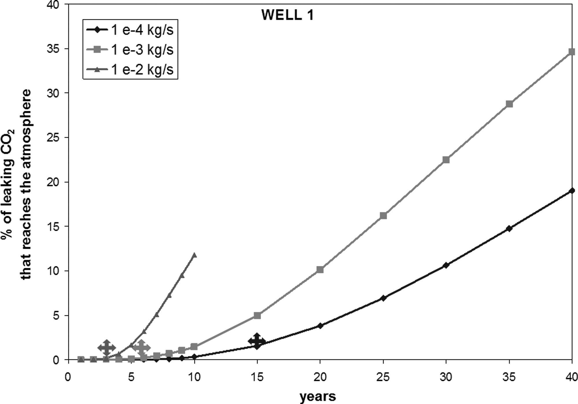
Total seepage history for the case with leakage at well 1. The thick crosses indicate the time of the first appearance of measurable levels of CO₂ seepage at the surface at any point in the domain.

FIG. 4.

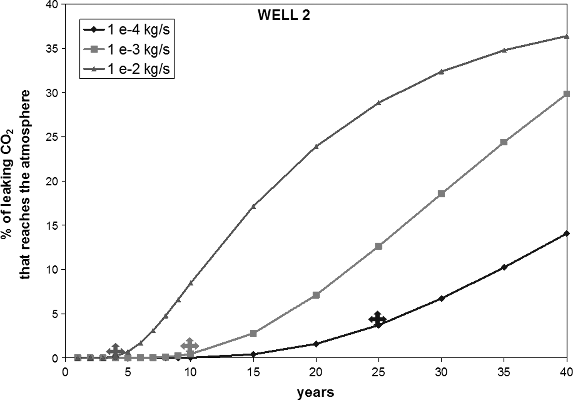
Total seepage history for the case with leakage at well 2. The thick crosses indicate the time of the first appearance of measurable levels of CO₂ seepage at the surface at any point in the domain.

Another observation from these figures is that, within the simulated time frame, none of the cases approaches a point where the entrance rate of CO₂ to the vadose zone from below is equal to the rate it is released to the atmosphere, which suggests a substantial accumulation in the vadose zone.

In Figs. 5 and 6, the ground surface seepage distribution for well 1 from a leakage of 10⁻⁴ kg/s is shown after 20 and 40 years, respectively. Figure 7 shows the ground-level distribution from a leakage of 10⁻⁴ kg/s from well 2 after 40 years. Keeping in mind that the (0,0) location for each case is the leaky well location, so the same coordinates in different figures do not refer to the same geographic location. Similarly, the elevation contours in each plot are measured from the elevation of the head of the leaking well. Indicated coordinates are in terms of meters. The gray-scale legend was adjusted so that any seepage below measuring capabilities is white.

FIG. 5.

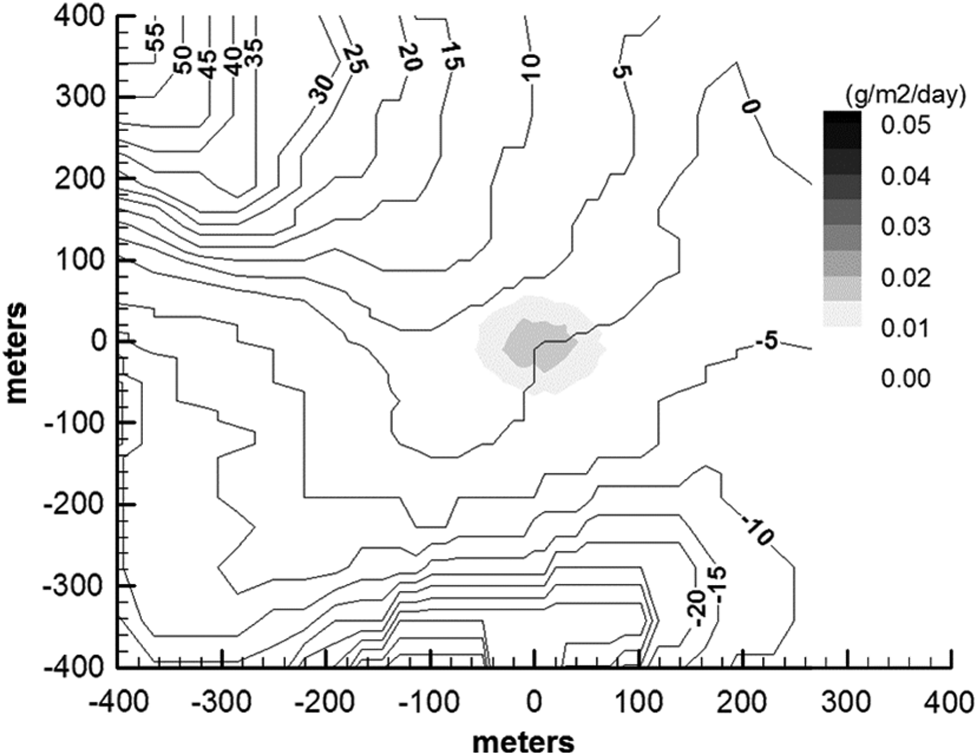
CO₂ seepage plot for well 1 (injection well) after 20 years.

FIG. 6.

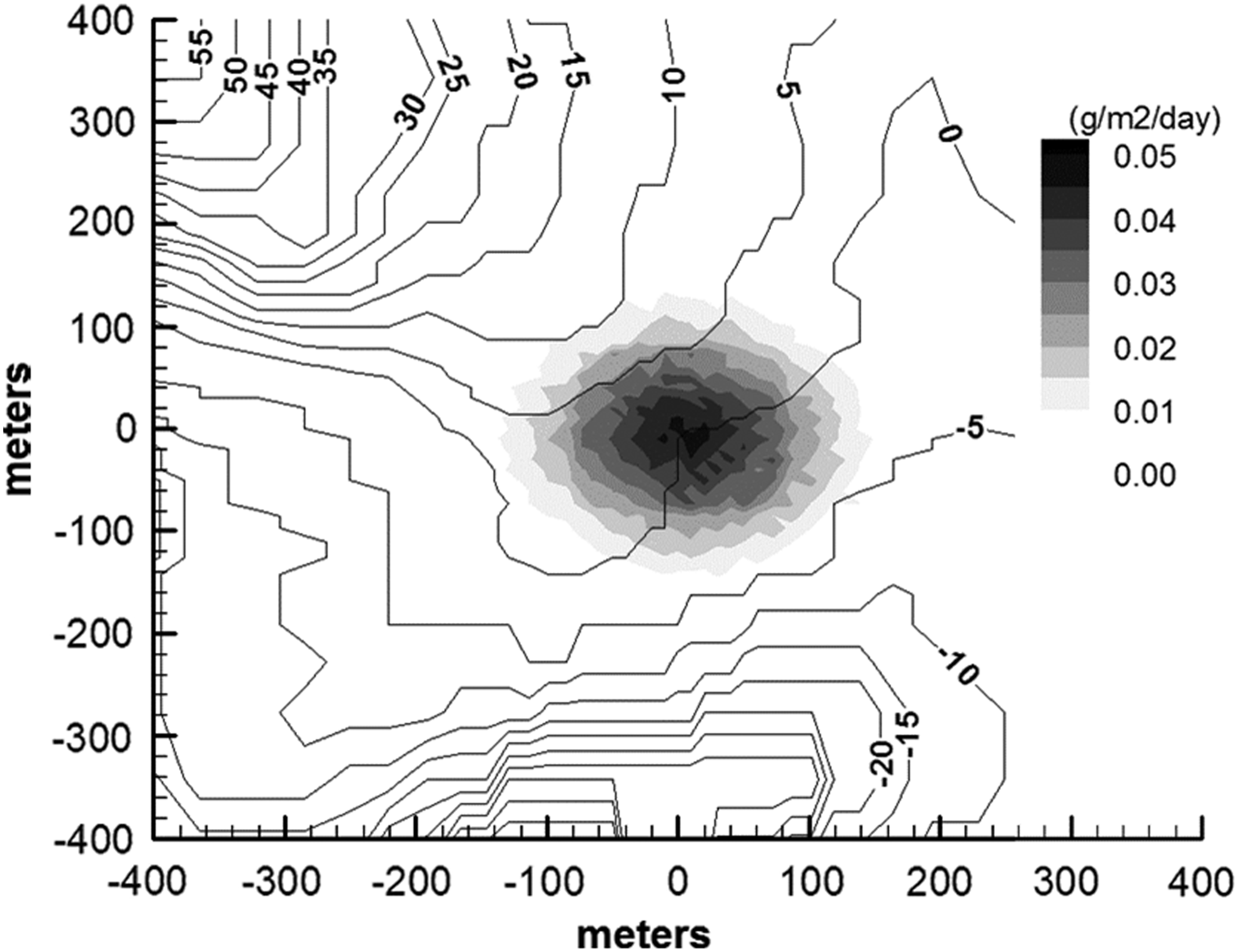
CO₂ seepage plot for well 1 (injection well) after 40 years.

FIG. 7.

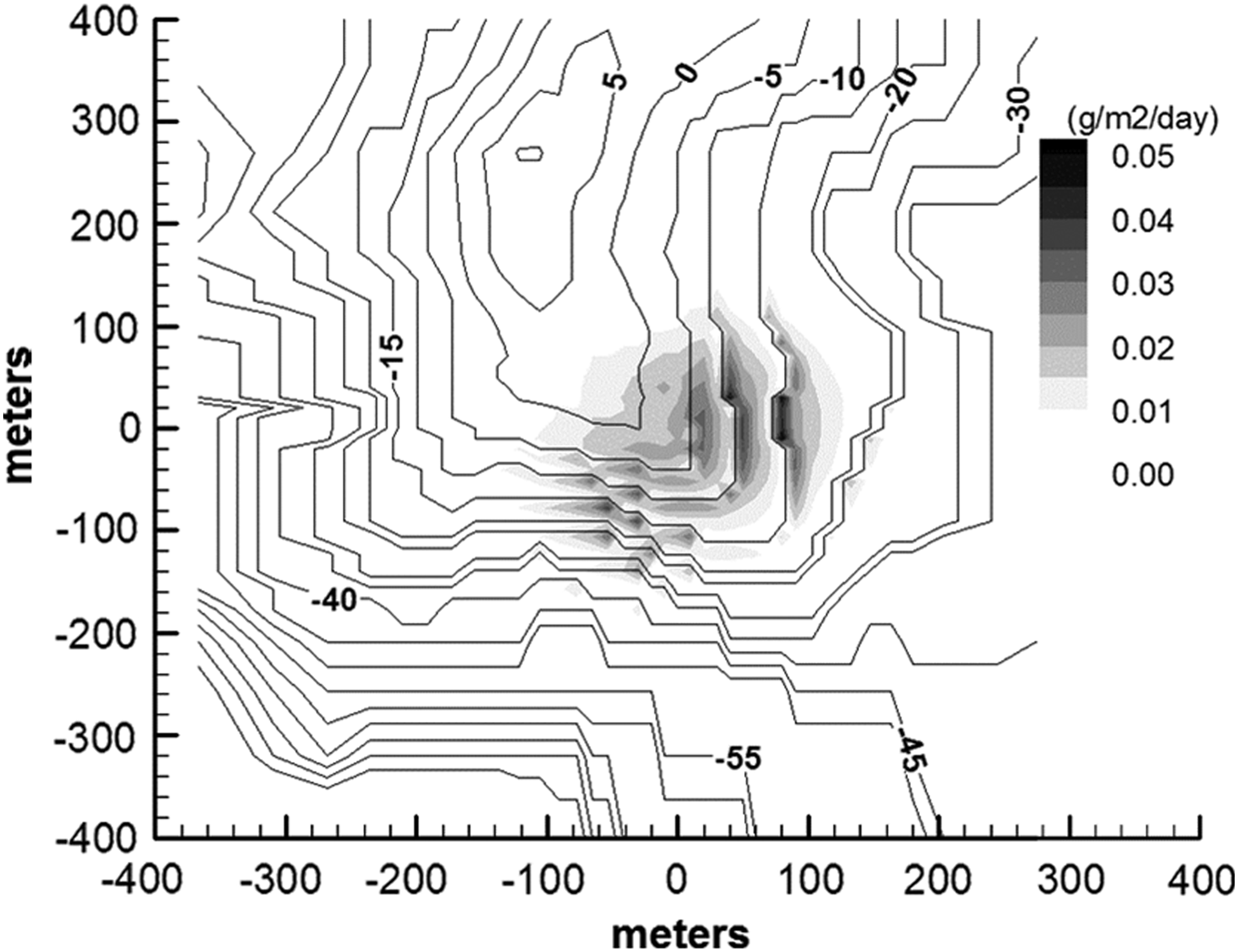
CO₂ seepage plot for well 2 (northwest production well) after 40 years.

For well 1, the vadose zone at the leaking well is about 80 m thick; whereas for well 2, the vadose zone is about 140 m thick. Consequently, after 20 years of leakage, although the plume expresses itself at measurable levels in well 1, it still remains unmeasurable for well 2; which is why a 20 year plot for well 2 was not included. Similarly, after 40 years of leakage, the seepage at the surface is more significant in well 1 than in well 2. It should be noted that “measurability” can change according to the technology used in the equipment. However, measurability does not necessarily warrant detection. When compared with a typical background CO₂ seepage flux of 7.6 g/(m²·day) in this kind of biome, none of the cases reveals values that are distinguishable from the natural background fluctuations in seepage. Although not shown here pictorially, increasing the leakage rate to 100 times (i.e., 10⁻² kg/s) for well 1 produced distinguishable seepage flux values (∼5 g/[m²·day]) within the first decade. Well 2 showed seepage values that are distinguishable from the background (∼3 g/[m²·day]) only after two decades with the same increased leakage rate of 10⁻² kg/s.

For well 1, which is located on a relatively flat surface, the seepage patterns are concentrated around the well. For well 2, which is located near the bank of a hill, the seepage pattern seems to be offset toward the embankment. Thus, the highest fluxes are observed not around the well head but on the hillside. This is due to the negative buoyancy of the CO₂ in the vadose zone, and the anisotropy of the rock type favoring horizontal migration.

The findings so far can be summarized as follows. For thick vadose zones, although “measurability” changes from one device to another, measurable levels of CO₂ flux at the surface occur years after the first entry to the vadose zone through the water table. Even then, measurability does not necessarily mean detectability, as the background fluctuations inhibit such a conclusion. This result still holds true even if much less background values are considered due to seasonal changes. Moreover, depending on the topography, the highest seepage fluxes may be displaced from the wellhead due to steepness and abrupt changes in the topography. Nevertheless, when looked at carefully, it is seen that the seepage flux distribution due to a leakage event covers an area with increased intensity at the inner locations. Moreover, this pattern is persistent over time and is at measurable levels. This is unlike a spatially haphazard or temporally periodic variation of flux in a natural background. Therefore, instead of comparing a single-point measurement at a specific time and place to background values, one could use statistical pattern recognition techniques to interpret spatially distributed measurements to come up with a satisfactory monitoring capability and sensitivity, without necessarily looking for single flux values that stand out of the natural background variation. The findings here not only highlight the need for statistical methods as discussed in Lewicki et al. (2005) and in Romanak et al. (2013) but also call for further improvement to address the challenges of thick vadose zones.

Summary

In summary, it is found that it may take several years, even decades, for a small leak into a thick vadose zone to produce measurable levels of CO₂ at the surface. In the simulations, the time required to reach such measurable levels is directly proportional to the vadose zone thickness and inversely proportional to the leakage rate, both nonlinearly. A great challenge is that even if the flux values are measurable, they are not necessarily distinguishable from the natural background. Therefore, a point flux measurement will not necessarily lead to leak detection. In order to overcome this issue, instead of using the comparison of single measurements to predetermined criteria, one can use statistical methods that detect patterns which are consistent over time and space. This will enable a more timely detection of leakages into the vadose zone, should they occur.

Footnotes

Acknowledgments

The authors thank Dustin Crandall from URS Corporation for his contribution to topographic data handling, Tom Wilson for his detailed geologic knowledge of the site, and Hema Siriwardane for the permeability measurements for the topsoil samples. As a part of the National Energy Technology Laboratory's Regional University Alliance (NETL-RUA), a collaborative initiative of the NETL, this technical effort was performed under the RES contract DE-FE0004000.

Author Disclosure Statement

No competing financial interests exist.

References

Annunziatellis

, Beaubien

S.E.

, Bigi

, Ciotoli

, Coltella

, and Lombardi

(2008). Gas migration along fault systems and through the vadose zone in the Latera caldera (central Italy): Implications for CO₂ geological storage. Int. J. Greenhouse Gas Control, 2, 353.

Bachu

, and Watson

T.L.

(2009). Review of failures for wells used for CO₂ and acid gas injection in Alberta, Canada. Energy Procedia, 1, 3531.

Barlet-Gouédard

, Rimmelé

, Goffé

, and Porcheria

(2007). Well technologies for CO₂ geological storage: CO₂-resistant cement. Oil Gas Sci. Technol., 62, 325.

Bernardo

, and de Vries

D.F.

(2011). Permanent shallow subsoil CO₂ flux chambers for monitoring of onshore CO₂ geological storage sites. Int. J. Greenhouse Gas Control, 5, 565.

Brown

, and Ferg

(2005). The use of lightweight cement slurries and downhole chokes on air-drilled wells. SPE Drill. Completion, 2, 123.

Busch

, Alles

, Gensterblum

, Prinz

, Dewhurst

D.N.

, Raven

M.D.

, Stanjek

, and Krooss

B.M.

(2008). Carbon dioxide storage potential of shales. Int. J. Greenhouse Gas Control, 2, 297.

Cable

J.M.

, Ogle

, Lucas

R.W.

, Huxman

T.E.

, Loik

M.E.

, Smith

S.D.

, Tissue

D.T.

, Ewers

B.E.

, Pendall

, Welker

J.M.

, Charlet

T.N.

, Cleary

, Griffith

, Nowak

R.S.

, Rogers

, Steltzer

, Sullivan

P.F.

, van Gestel

N.C.

(2011). The temperature responses of soil respiration in deserts: A seven desert synthesis. Biogeochemistry, 103, 71.

Carey

J.W.

, Wigand

, Chipera

S.J.

, WoldeGabriel

, Pawar

, Lichtner

P.C.

, Wehner

S.C.

, Raines

M.A.

, and Guthrie

G.D.

(2007). Analysis and performance of oil well cement with 30 years of CO₂ exposure from the SACROC unit, west Texas, USA. Int. J. Greenhouse Gas Control, 1, 75.

Clarkson

C.R.

, Rahmanian

, Kantzas

, and Morad

(2010). Relative permeability of CBM reservoirs: Controls on curve shape. Int. J. Coal Geol., 88, 204.

10.

Economides

M.J.

, Oligney

R.E.

, and Lewis

P.E.

(2012). U.S. natural gas in 2011 and beyond. J. Nat. Gas Sci. Eng., 8, 2.

11.

Feng

, Hongming

, Yingfeng

, Gao

, and Xijin

(2009). Damage evaluation for water-based underbalanaced drilling in low-permeability and tight sandstone gas reservoirs. Petrol. Explor. Dev., 36, 113.

12.

Gentzis

(2000). Subsurface sequestration of carbon dioxide—An overview from an Alberta (Canada) perspective. Int. J. Coal Geol., 43, 287.

13.

Harpalani

, and Chen

(1995). Estimation of changes in fracture porosity of coal with gas emission. Fuel, 74, 1491.

14.

Harpalani

, and Mitra

(2010). Impact of CO₂ injection on flow behavior of coalbed methane reservoirs. Transp. Porous Med., 82, 141.

15.

Hart

B.S.

(2006). Seismic expression of fracture-swarm sweet spots, Upper Cretaceous tight-gas reservoirs, San Juan basin. AAPG Bull., 90, 1519.

16.

Huerta

N.J.

, Bryant

S.L.

, Strazisar

B.R.

, and Hesse

(2011). Dynamic alteration along a fractured cement/cement interface: Implications for long term leakage risk along a well with an annulus defect. Energy Procedia, 4, 5398.

17.

Kolenkovic

, Saftic

, and Peresin

(2013). Regional capacity estimates for CO₂ geological storage in deep saline aquifers–Upper Miocene sandstones in the SW part of the Pannonian basin. Int. J. Greenhouse Gas Control, 16, 180.

18.

Koornneef

, Ramirez

, Turkenburg

, and Faaij

(2012). The environmental impact and risk assessment of CO₂ capture, transport and storage—An evaluation of the knowledge base. Prog. Energy Combust. Sci., 38, 62.

19.

Korre

, Shi

J.Q.

, Imrie

, Grattoni

, and Durucan

(2007). Coalbed methane reservoir data and simulator parameter uncertainty modeling for CO₂ storage performance assessment. Int. J. Greenhouse Gas Control, 1, 492.

20.

Kutchko

B.G.

, Strazisar

B.R.

, Dzombak

D.A.

, Lowry

G.V.

, and Thaulow

(2007). Degradation of well cement by CO₂ under geologic sequestration conditions. Environ. Sci. Technol., 41, 4787.

21.

Le Guen

, Poupard

, and Loizzo

(2009). Optimization of plugging design for well abandonment—Risk management of long-term well integrity. Energy Procedia, 1, 3587.

22.

Lewicki

J.L.

, Hilley

G.E.

, and Oldenburg

C.M.

(2005). An improved strategy to detect CO₂ leakage for verification of geologic carbon sequestration. Geophys. Res. Lett., 32, L19403.

23.

Lewicki

J.L.

, Oldenburg

C.M.

, Dobeck

, and Spangler

(2007). Surface CO₂ leakage during two shallow subsurface CO₂ releases. Geophy. Res. Lett., 34, L24402.

24.

Mainguy

, Longuemare

, Audibert

, and Lécolier

(2007). Analyzing the risk of well plug failure after abandonment. Oil Gas Sci. Technol. 62/3, 311.

25.

Marroquin

I.D.

, and Hart

B.S.

(2004). Seismic attribute-based characterization of coalbed methane reservoirs: An example from the Fruitland formation, San Juan basin, New Mexico. AAPG Bull., 88, 1603.

26.

Mathieson

, Wright

, Roberts

, and Ringrose

(2009). Satellite imaging to monitor CO₂ movement at Krechba, Algeria. Energy Procedia, 1, 2201.

27.

Mavor

M.J.

, and Vaughn

J.E.

(1998). Increasing coal absolute permeability in the San Juan basin Fruitland formation. SPE Reservoir Eval. Eng., 1, 201.

28.

Mazumder

, and Wolf

K.H.

(2008). Differential swelling and permeability change of coal in response to CO₂ injection for ECBM. Int. Journ. Coal Geol., 74, 123.

29.

Metz

, Davidson

, de Coninck

, Loos

, and Meyer

(Eds.) (2005). IPCC Special Report on Carbon Capture and Storage. Cambridge, United Kingdom: Cambridge University Press.

30.

Ogretim

, Gray

D.D.

, and Bromhal

G.S.

(2009). Effects of topography induced pressure variation on the near-surface migration of a potential CO₂ leak. Energy Procedia, 1, 2341.

31.

Oldenburg

C.M.

, and Unger

A.J.A.

(2004). Coupled vadose zone and atmospheric surface-layer transport of carbon dioxide from geologic carbon sequestration sites. Vadose Zone J., 3, 848.

32.

Oldenburg

C.M.

, and Unger

A.J.A.

(2003). On leakage and seepage from geologic carbon sequestration sites: Unsaturated zone attenuation. Vadose Zone J., 2, 287.

33.

Ozdemir

(2009). Modeling of coal bed methane (CBM) production and CO₂ sequestration in coal seams. Int. J. Coal Geol., 77, 145.

34.

Palmer

(2010). Coalbed methane completions: A world view. Int. J. Coal Geol., 82, 184.

35.

Palmer

(2009). Permeability changes in coal: Analytical modeling. Int. J. Coal Geol., 77, 119.

36.

Pan

, Lewicki

J.L.

, Oldenburg

C.M.

, and Fisher

M.L.

(2010). Time-windows-based filtering method for near-surface detection of leakage from geologic carbon sequestration sites. Env. Earth Sci., 60, 359.

37.

Patroni

J.M.

(2007). Lifetime of a natural gas storage well assessment of well-field maintenance cost. Oil Gas Sci. Technol., 62, 297.

38.

Pawar

, Watson

T.L.

, and Gable

C.W.

(2009). Numerical simulation of CO₂ leakage through abandoned wells: Model for an abandoned site with observed gas migration in Alberta, Canada. Energy Procedia, 1, 3625.

39.

Pillalamarry

, Harpalani

, and Liu

(2011). Gas diffusion behavior of coal and its impact on production from coalbed methane reservoirs. Int. J. Coal Geol., 86, 342.

40.

Pruess

, Oldenburg

C.M.

, and Moridis

G.J.

(1999). TOUGH2 User's Guide Version 2. LBNL Report LBNL-43134.

41.

Rahman

M.K.

, Suarez

Y.A.

, Chen

, and Rahman

S.S.

(2007). Unsuccessful hydraulic fracturing cases in Australia: investigation into causes of failures and their remedies. J. Pet. Sci. Eng., 57, 70.

42.

Romanak

, and Sherk

G.W.

(2013). Protocol for Response to Claims of CO₂ Leakage Developed at The Kerr Farm: Weyburn-Midale Oilfield. Presented at the 7th Trondheim Conference on CO2 Capture, Transport and Storage, June 4–6, Trondheim, Norway.

43.

Romanak

, Dobeck

, Dixon

, and Spangler

(2013). Potential for a process-based monitoring method above geologic carbon storage sites using dissolved gases in freshwater aquifers. Procedia Earth Planet. Sci., 7, 746.

44.

Shi

J.-Q.

, and Durucan

(2010). Exponential growth in San Juan basin Fruitland coalbed permeability with reservoir drawdown: Model match and new insights. SPE Reservoir Eval. Eng., 13, 914.

45.

Shuck

E.L.

, Davis

T.L.

, and Benson

R.D.

(1996). Multicomponent 3-D characterization of a coalbed methane reservoir. Geophysics, 61, 315.

46.

Siriwardane

H.J.

, Bowes

B.D.

, Bromhal

G.S.

, Gondle

R.K.

, Wells

A.W.

, Strazisar

B.R.

(2012). Modeling of CBM production, CO₂ injection, and tracer movement at a field CO₂ sequestration site. Int. J. Coal Geol., 96, 120.

47.

Spangler

L.H.

, Dobeck

L.M.

, Repasky

K.S.

, Nehrir

A.R.

, Humphries

S.D.

, Barr

J.L.

, Keith

C.J.

, Shaw

J.A.

, Rouse

J.H.

, Cunningham

A.B.

, Benson

S.M.

, Oldenburg

C.M.

, Lewicki

J.L.

, Wells

A.W.

, Diehl

J.R.

, Strazisar

B.R.

, Fessenden

J.E.

, Rahn

T.A.

, Amonette

J.E.

, Barr

J.L.

, Pickles

W.L.

, Jacobson

J.D.

, Silver

E.A.

, Male

E.J.

, Rauch

H.W.

, Gullickson

K.S.

, Trautz

, Kharaka

, Birkholzer

, and Wielopolski

(2010). A shallow subsurface controlled release facility in Bozeman, Montana, USA, for testing near surface CO₂ detection techniques and transport models. Environ. Earth Sci., 60, 227.

48.

Strazisar

B.R.

, Wells

A.W.

, Diehl

J.R.

, Hammack

R.W.

, and Veloski

G.A.

(2009). Near surface monitoring for the ZERT shallow CO₂ injection project. Int. J. Greenhouse Gas Control, 3, 736.

49.

Sun

, Gao

, and Zhu

(2012). Models & tests of casing wear in drilling for oil & gas. J. Nat. Gas Sci. Eng., 4, 44.

50.

Sun

A.Y.

, Zeidouni

, Nicot

J-P.

, Lu

, and Zhang

(2013). Assessing leakage detectability at geologic CO₂ sequestration sites using the probabilistic collocation method. Adv. Water Resour., 56, 49.

51.

van der Kuip

M.D.C.

, Benedictus

, Wildgust

, and Aiken

(2011). High-level integrity assessment of abandoned wells. Energy Procedia, 4, 5320.

52.

Wang

(2009). The state-of-the-art in natural gas production. J. Nat. Gas Sci. Eng., 1, 14.

53.

Wilson

T.H.

, Wells

, and Peters

(2012). Fracture and 3D seismic interpretations of the fruitland formation and cover strata: Implications for CO₂ retention and tracer movement, San Juan Basin Pilot Test. Int. J. Coal Geol., 99, 35.

54.

Yang

Ya-Mei

, Small

, Ogretim

, Gray

D.D.

, Bromhal

G.S.

, Strazisar

, and Wells

(2011). Probabilistic design of a near surface CO₂ leak detection system. Environ. Sci. Tech., 45, 6380.