Statistical Model for Scaling and Corrosion Potentials of Cooling-System Source Waters

Abstract

Determination of make-up cooling water scaling and corrosion potentials for power plants is essential to prevent cooling system fouling challenges linked to source water quality. In this study, a statistical model is proposed to evaluate the probability that scaling or corrosion could occur. These probabilities were determined from derived distributions for the Langelier saturation index (LSI) and the aggressive index (AI), computed from a fitted joint normal distribution for pH, log[Ca²⁺], log([Ca²⁺]+[Mg²⁺]), and log[Alk]. In most cases only one outcome (scaling or corrosion) exhibited a probability of concern, though highly variable source waters could exhibit significant probability for both. To illustrate application of the method, freshwater and treated municipal wastewater samples collected from the western Pennsylvanian region were analyzed for alkalinity, pH, [Mg²⁺] and [Ca²⁺] concentrations. The LSI and AI were calculated using the measured characteristics of the water samples, and their observed distributions were compared to the derived normal distributions for each. This study used the uncertainty associated with water quality inputs to evaluate the uncertainty of scaling and corrosion potentials, and provides a practical approach for power plant operators to evaluate the uncertainty associated with scaling and corrosion indices of cooling waters without use of expensive software or complicated coding.

Introduction

Since 1965, freshwater withdrawal and use in the United States has been greatly influenced by the power-generation industry, especially by the generation of thermoelectric power. According to the U.S. Geological Survey (Kenny et al., 2009), ∼41% of water withdrawal in the United States is for thermoelectric cooling systems, and data from the National Renewable Energy Laboratory (Macknick, 2012) indicate that 41% of U.S. water withdrawal and 3% of U.S. water consumption occur in thermoelectric power production.

Two common types of wet cooling systems currently employed in thermoelectric power plants include once-through and recirculating towers. In once-through cooling systems, cooling water circulated once through the system is directly discharged back to the source. In a recirculating cooling system (shown in Fig. 1), cooling water is circulated from the make-up water basin to the heat exchanger and then to the cooling tower and back to the basin completing one cycle of concentration (CoC). During each flow cycle, evaporation and drift in the cooling tower cause a decrease in the cooling water quantity, which leads to an increase in the ionic concentrations of the make-up water. To maintain the CoC=4 or 5 and to ensure that the heat exchanger functions efficiently with minimal fouling, it is necessary for the influent make-up water to have low solid/ion concentrations and organic matter (Vidic and Dzombak, 2009). The focuses of this article are inorganic scale formation caused by high calcium concentration and high alkalinity, and corrosion caused by low pH. However, organic matters in cooling water also play an important role in heat exchanger fouling, because organic matters are food source for microorganisms and the growth of microorganisms results in biofilm formation and subsequent clogging of heat exchanger and reduction of heat-exchange efficiency (Cloete et al., 1998; Meesters et al., 2003).

FIG. 1.

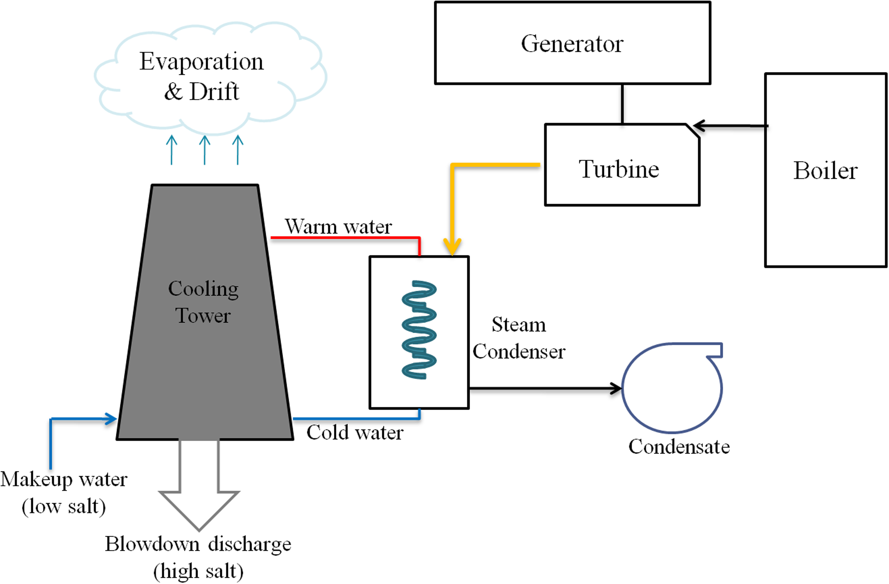
Schematic of coal-fired power plant cooling system (Vidic and Dzombak, 2009).

About 43% of U.S. thermoelectric plants utilize once-through cooling configurations (Vidic and Dzombak, 2009), and the resulting effects on instream flows and temperatures could lead to significant ecosystem impacts. To regulate the effects on aquatic life, the U.S. Clean Water Act 316 (b) (U.S. EPA, 2010) is driving power plants to implement recirculating cooling towers and seek alternative sources for cooling water make-up. Gross withdrawals from natural water systems can be reduced substantially by replacing once-through cooling systems with recirculating cooling systems. Additionally, alternative sources of make-up water can further reduce freshwater withdrawal for thermoelectric power generation. The reclamation of municipal wastewater (MWW) in cooling systems represents a viable, long-term solution to the challenges presented by growing municipal, industrial, and agricultural demands for water (Liu et al., 2012). Use of treated MWW as make-up water for cooling in power plants has been in full-scale operation for several decades (Ehrhardt et al., 1986). Secondary-treated wastewaters from publicly operated treatment works (POTWs) were reported to be easily accessible and can satisfy ∼75% of the cooling water needs for electricity generation (Vidic and Dzombak, 2009).

Using a freshwater or treated wastewater source in a cooling system requires evaluation of the scaling and corrosion potentials of the waters under higher CoC recirculation, since the presence of elevated total dissolved solid (TDS) levels leads to accelerated solid precipitation or reaction with the heat exchanger metal when water is concentrated due to evaporation. The cooling system may encounter various problems related to water properties, such as scale formation, corrosion, and microorganism growth (Zdaniuk et al., 2006; Chien et al., 2009; Buyuksagis and Erol, 2012). Specifically, if water quality indices are not in their desired range (e.g., high calcium hardness, high alkalinity, too high or too low pH, and high temperature), tower scaling and corrosion problems may occur (Cheremisinoff and Cheremisinoff, 1981). Previously, pilot-scale cooling system studies have been carried out to evaluate the scaling and corrosion potentials of alternative sources of make-up water (Swart and Engelbrecht, 2004; Li et al., 2011; Chien, et al., 2012; Liu et al., 2012). These studies have reported the need for tertiary and/or chemical treatment for effective reuse of degraded water sources (e.g., sewage or industrial wastewater) for cooling. These studies provide a detailed and necessary feasibility analysis, but to test multiple sources simultaneously at the preliminary stage, the use of pilot-scale systems can be time consuming and resource intensive. A screening model that considers the inherent variation in water quality from a given source is proposed here to provide an initial prioritization of source waters for these more detailed studies.

Evaluation of scaling and corrosion potentials can now be conducted with the use of scale and corrosion modeling software (e.g., WaterCycle^® Rx) (French Creek Software, Inc., 1999). WaterCycle Rx allows users to evaluate scaling and corrosion potentials for common scalants over the range of water chemistry, temperature, and pH anticipated in an operational cooling system. Results of scaling and corrosion indices can be presented in graphical or tabular form (French Creek Software, Inc., 1999). The software evaluates the uncertainty of scaling and corrosion indices by repeating calculations of these indices using a range for each input parameter (e.g., if a range of 6–8 for pH is given, then the software will calculate the values of scaling and corrosion indices using a set of pH values between 6 and 8). By doing that, ranges of both scaling and corrosion indices can be obtained, and the maximum and minimum values of the ranges reflect uncertainties of scaling and corrosion indices.

Different from WaterCycle Rx, this article uses statistical analysis to evaluate uncertainties of scaling and corrosion indices. To be specific, cumulative distribution functions (CDFs) of both scaling index (the Langelier saturation index [LSI]) and corrosion index (aggressive index [AI]) were calculated. The calculation was based on water quality parameters obtained from water sampling. The CDFs can then be used to quantify uncertainties of both Langelier index and AI. In summary, this article presents a methodology to quantify uncertainties associated with LSI and AI with the use of statistics and probability distribution, which is different from commonly used scale and corrosion modeling software.

In this study, the LSI and the AI are used to identify the corrosion and scaling potential of river water (Monongahela River in southwestern Pennsylvania) and secondary- and tertiary-treated wastewater (Franklin Township Municipal Sanitation Authority [FTMSA] in Murrysville, southwestern PA). Scaling and corrosion potentials of the Monongahela River water and the secondary and tertiary wastewater from FTMSA is investigated because the Monongahela River basin and FTMSA are located in a region with a high density of power plants (see Fig. 2). Nine power plants along the Monongahela River have already used river water as cooling water, and the wastewater from FTMSA can be used as cooling water in the future to offset the cooling water withdrawal from river water to run the eight power plants within 20-mile radius of FTMSA. The two sampling locations along Monongahela River and the location of FTMSA can be seen in Fig. 2.

FIG. 2.

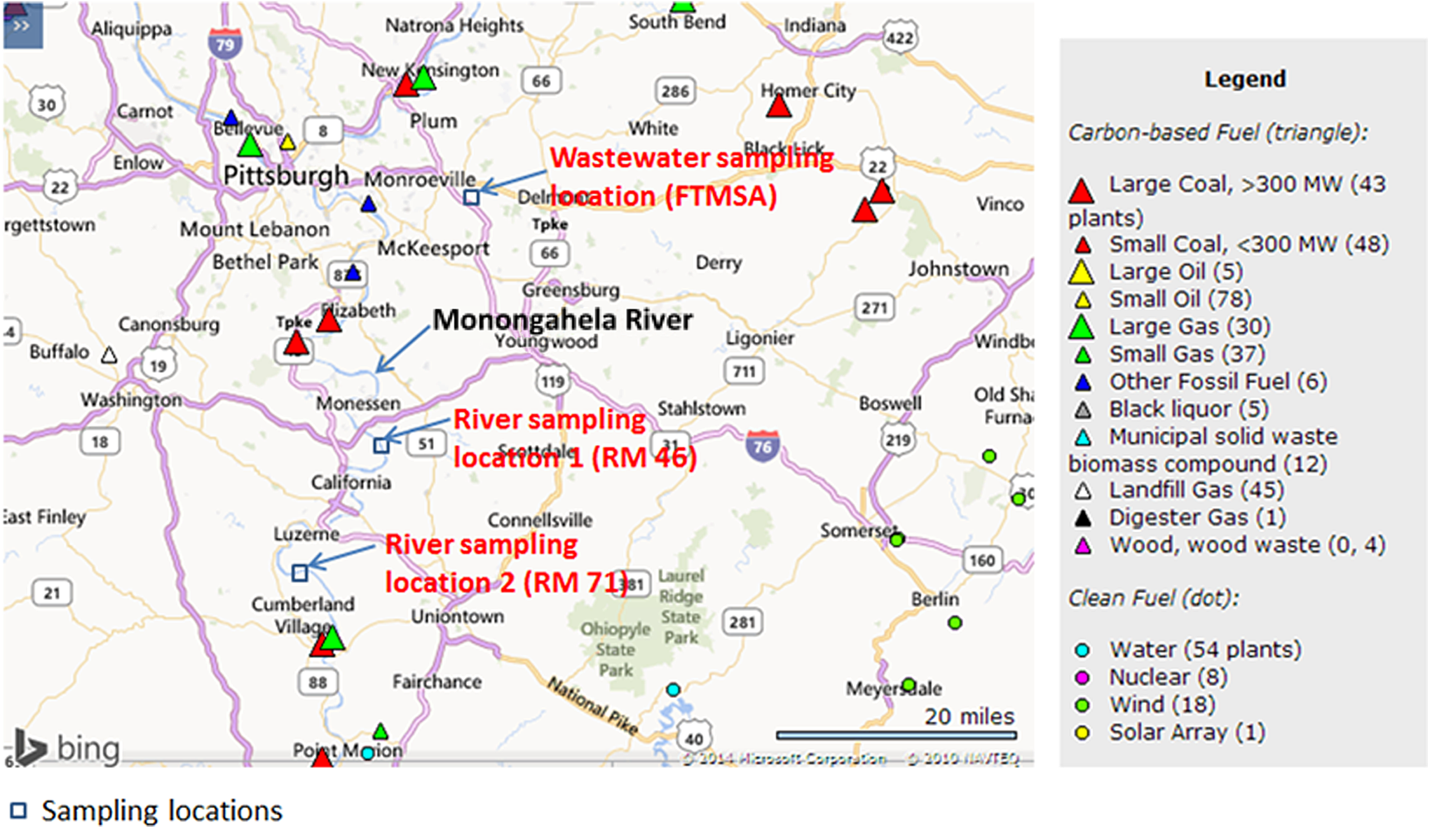
Map showing power plants close to Monongahela River and FTMSA, and two sampling locations along Monongahela River (modified from U.S. EPA, 2014).

LSI reflects the equilibrium pH of water with respect to calcium and alkalinity. This index is used to indicate the tendency of both corrosion and the deposition of scale (Langelier, 1936; U.S. EPA, 2009). The AI is sometimes substituted for the LSI as an indicator of corrosivity of water and is derived from the actual pH, total hardness, and total alkalinity (Hach, 2009). Scaling and corrosion in the cooling system and fouling in the heat exchanger are extremely complex phenomena and the use of scaling and corrosion indices may not fully describe the time-dependent nature of these processes (Sheikh et al., 2001). Nonetheless, the LSI and AI are broadly used to help understand possible causes of corrosion (Taghipour et al., 2012).

The calculations of LSI and AI are based on the pH, alkalinity, calcium concentration, total hardness values, and temperature measured from water samples, and the results of LSI and AI are always associated with variability and uncertainty. To address these issues and obtain a reliable correlation between influent water quality and the tendency for scaling/corrosion, the results of LSI and AI may be expressed in a probabilistic way. The objectives of this study are (1) to demonstrate a statistical approach to evaluate the probability of cooling water causing scaling and corrosion, using fitted distributions for the water quality inputs (i.e., pH, alkalinity, calcium concentration, and total hardness) included in the scaling and corrosion index equations, and (2) to use this approach to evaluate the probability of river water and wastewater samples causing scaling and corrosion in an area with high power plant density in southwestern Pennsylvania. The novelty of this approach is that this approach correlates the uncertainty associated with water quality inputs with the uncertainty of scaling and corrosion indices without use of expensive software or complicated calculation. This approach is practical and can be used by power plant operators as a standard method to evaluate scaling and corrosion potentials of their cooling water.

Statistical and Experimental Analysis

Model formulation

To calculate LSI and AI in a probabilistic way, a joint lognormal distribution was fit to observed co-occurrence of source water alkalinity, calcium, hardness, and hydrogen ion concentration (equivalent to a normal distribution for pH), leading to derived normal distributions for the computed LSI and AI. From these derived distributions, we are able to directly estimate the probabilities that these indices are either above or below critical values.

LSI for scaling potential

The LSI is based on the solubility of calcium carbonate and the potential of the water to form scale (Langelier, 1936; Assembly of Life Sciences [U.S.], 1982). The LSI was chosen to characterize scaling potential because of its ease of calculation and the wide application of this index to different types of waters and to different water usage conditions around the world (Assembly of Life Sciences [U.S.], 1982; Rafferty, 1999; Luo et al., 2009; Gupta et al., 2011; Kinsela et al., 2012). The expression for LSI is written as (Ahmad, 2006) follows: \documentclass{aastex}\usepackage{amsbsy}\usepackage{amsfonts}\usepackage{amssymb}\usepackage{bm}\usepackage{mathrsfs}\usepackage{pifont}\usepackage{stmaryrd}\usepackage{textcomp}\usepackage{portland, xspace}\usepackage{amsmath, amsxtra}\pagestyle{empty}\DeclareMathSizes{10}{9}{7}{6}\begin{document} \begin{align*}LSI = pH - pH_s \tag{1}\end{align*} \end{document}

where pH_s is the saturation pH (the pH at which the carbonate alkalinity and [Ca²⁺] are in equilibrium with CaCO₃), and pH is the actual pH of the water.

The pH_s is calculated as follows (Ahmad, 2006): \documentclass{aastex}\usepackage{amsbsy}\usepackage{amsfonts}\usepackage{amssymb}\usepackage{bm}\usepackage{mathrsfs}\usepackage{pifont}\usepackage{stmaryrd}\usepackage{textcomp}\usepackage{portland, xspace}\usepackage{amsmath, amsxtra}\pagestyle{empty}\DeclareMathSizes{10}{9}{7}{6}\begin{document} \begin{align*}{ \rm pH}_{ \rm s} = A + B - \log [ { \rm Ca}^{2 + } ] - \log [ { \rm Alk} ] \tag{2}\end{align*} \end{document}

where log[Ca²⁺] is the (base 10) logarithm of Ca²⁺ in mg/L as CaCO₃ and log[Alk] is the logarithm of total alkalinity in mg/L as CaCO₃. A is a parameter describing the impact of water temperature on the scaling potential, and B is a parameter describing the impact of the TDS concentration on the scaling potential. A can be expressed as a function of temperature. \documentclass{aastex}\usepackage{amsbsy}\usepackage{amsfonts}\usepackage{amssymb}\usepackage{bm}\usepackage{mathrsfs}\usepackage{pifont}\usepackage{stmaryrd}\usepackage{textcomp}\usepackage{portland, xspace}\usepackage{amsmath, amsxtra}\pagestyle{empty}\DeclareMathSizes{10}{9}{7}{6}\begin{document} \begin{align*}A = - 0.0183T + 2.5127 \tag{3}\end{align*} \end{document}

where T is temperature in the unit of °C. Details about how the expression was obtained can be seen in Supplementary Data.

B can be expressed as a function of TDS: \documentclass{aastex}\usepackage{amsbsy}\usepackage{amsfonts}\usepackage{amssymb}\usepackage{bm}\usepackage{mathrsfs}\usepackage{pifont}\usepackage{stmaryrd}\usepackage{textcomp}\usepackage{portland, xspace}\usepackage{amsmath, amsxtra}\pagestyle{empty}\DeclareMathSizes{10}{9}{7}{6}\begin{document} \begin{align*}B = 0.19 \times \log ( { \rm TDS} + 100 ) + 9.3351 \tag{4}\end{align*} \end{document}

where TDS is TDS concentration in the unit of mg/L. Details about how the expression was obtained can be seen in Supplementary Data.

Equation (4) shows that the change in TDS only results in a small change in B. For example, a TDS value of 400 mg/L yields a B value of 9.86, and a TDS value of 1,000 mg/L yields a B value of 9.91. Therefore, only one value is assigned for B (B=9.86, corresponding to a TDS of 400 mg/L) in the following calculations.

An LSI>0 means that the solution is supersaturated with CaCO₃ and will tend to form scale; an LSI<0 means that the water is undersaturated with CaCO₃ and there will be no scale formation (Ahmad, 2006). Here “supersaturated” means [Ca²⁺][CO₃²⁻]>K_sp(CaCO₃) and CaCO₃ tends to precipitate; “undersaturated” means [Ca²⁺][CO₃²⁻]<K_sp(CaCO₃) and CaCO₃ would not precipitate. It is important to note that an LSI value slightly higher than zero is actually beneficial for the pipeline, as the formation of a small amount of scale will not block the pipeline and is protective against corrosion. Nonetheless, a value of LSI=0 is usually considered to be the threshold where scaling begins to occur, and values of LSI>0 are thus assumed to indicate this concern. Note that Equations (1) and (2) may be combined to yield: \documentclass{aastex}\usepackage{amsbsy}\usepackage{amsfonts}\usepackage{amssymb}\usepackage{bm}\usepackage{mathrsfs}\usepackage{pifont}\usepackage{stmaryrd}\usepackage{textcomp}\usepackage{portland, xspace}\usepackage{amsmath, amsxtra}\pagestyle{empty}\DeclareMathSizes{10}{9}{7}{6}\begin{document} \begin{align*}{ \rm LSI = pH} - ( { A + B} ) + \log [ { \rm Ca}^{2 + } ] + \log [ Alk ] \tag{5}\end{align*} \end{document}

and, for (A+B)=−0.0183T+12.37, we obtain \documentclass{aastex}\usepackage{amsbsy}\usepackage{amsfonts}\usepackage{amssymb}\usepackage{bm}\usepackage{mathrsfs}\usepackage{pifont}\usepackage{stmaryrd}\usepackage{textcomp}\usepackage{portland, xspace}\usepackage{amsmath, amsxtra}\pagestyle{empty}\DeclareMathSizes{10}{9}{7}{6}\begin{document} \begin{align*}LSI = pH + 0.0183T - 12.37 + \log [ Ca^{2 + } ] + \log [ Alk ] \tag{6}\end{align*} \end{document}

It is important to note that the water undergoes temperature increase when the water goes through the cooling system, which impacts the scale formation potential. As a result, it is recommended to measure the temperature of the cooling water in the cooling system and to choose an A value that is consistent with the measured temperature when applying the model. In this study, we chose three temperature points (T=10°C, 20°C, and 30°C) and calculated probability distributions of LSI at these temperature points, so as to investigate the impact of temperature change on the scaling potential.

Aggressive index

AI, Ryzner index, and Riddick corrosion index are three indices that are most widely used to evaluate the corrosion potential of a given water sample (Ahmad, 2006). AI and Ryzner index have the same inputs (pH, alkalinity, calcium hardness, TDS, and temperature) and are widely used due to easiness to use. Riddick corrosion index requires more inputs (i.e., nitrate ion concentration, CO₂ concentration, dissolved O₂ concentration, Cl⁻ concentration, and dissolved SiO₂ concentration) for calculation, and may only be considered when the data of the required inputs are available. In this study, the AI is used. The expression for AI is (Zuane, 1997) as follows: \documentclass{aastex}\usepackage{amsbsy}\usepackage{amsfonts}\usepackage{amssymb}\usepackage{bm}\usepackage{mathrsfs}\usepackage{pifont}\usepackage{stmaryrd}\usepackage{textcomp}\usepackage{portland, xspace}\usepackage{amsmath, amsxtra}\pagestyle{empty}\DeclareMathSizes{10}{9}{7}{6}\begin{document} \begin{align*}{ \rm AI} = { \rm pH} + \log [ ( { \rm Alk} ) ( H ) ] \tag{7}\end{align*} \end{document}

where (Alk) has been defined previously and H is total hardness in mg/L as CaCO₃. In our study, H=[Ca²⁺]+[Mg²⁺]. Expanding the last (logarithmic) term we obtain the following equation: \documentclass{aastex}\usepackage{amsbsy}\usepackage{amsfonts}\usepackage{amssymb}\usepackage{bm}\usepackage{mathrsfs}\usepackage{pifont}\usepackage{stmaryrd}\usepackage{textcomp}\usepackage{portland, xspace}\usepackage{amsmath, amsxtra}\pagestyle{empty}\DeclareMathSizes{10}{9}{7}{6}\begin{document} \begin{align*}{ \rm AI} = { \rm pH} + \log [ { \rm Alk} ] + \log [ { \rm Ca}^{2 + } + { \rm Mg}^{2 + } ] \tag{8}\end{align*} \end{document}

An AI <10 means that the water sample is very corrosive; an AI between 10 and 12 means that the water is moderately corrosive and an AI>12 indicates that the water is not corrosive.

The underlying statistical model assumes lognormal distributions for the hydrogen ion concentration, calcium ion concentration, and alkalinity, resulting in normal distributions for pH, log[Ca²⁺], and log[Alk]. The assumption is realistic because the lognormal distribution has been found to provide a good approximation for chemical concentrations in air, soil, and water (Ott, 1990), for example, in describing the variation of chemical concentrations in groundwater (Bjerg and Christensen, 1992), and in lakes impacted by acid deposition (e.g., Small et al., 1988). If pH, log[Ca²⁺], and log[Alk] follow normal distribution, then both LSI and AI would follow normal distribution as well, because the sum of multiple variables following normal distribution is normally distributed. To investigate how well the LSI and AI data can be fit by normal distribution, the goodness-of-fit of normal distribution to both LSI and AI data was examined and results are presented in “Results and Discussion” section.

To demonstrate application of the statistical model, data for pH, alkalinity, [Ca²⁺], and [Mg²⁺] were collected from two river water sampling locations (river mile 46 [RM 46] and river mile 71 [RM 71]) and one wastewater treatment plant (FTMSA, Murrysville, PA) in southwestern Pennsylvania. Waters collected at FTMSA included secondary-treated MWW (MWW-2) and tertiary-treated MWW (MWW-3). Data collected were used in the statistical model to calculate the probabilities of scaling and corrosion of water samples. A total of seven samples were collected at each sampling location and all samples were collected from April 17, 2012, to August 6, 2012, at an average frequency of one sample per 18 days. pH values of samples were measured by a pH meter, alkalinity values of samples were measured by H₂SO₄ titration, and [Ca²⁺] and [Mg²⁺] values were measured by atomic absorption spectrophotometry. Details of sample collection and raw data can be found in Supplementary Data (Supplementary Table S1). Calculated LSI and AI values for each sample with the use of Equations (4) and (6) are presented in Table 1 (given a temperature of 20°C). It is important to note that the data collected mainly serve to demonstrate how the statistical model is applied. The number of samples collected at each sampling location may not be large enough to derive scaling and corrosion potentials for the corresponding waters, and the characteristics of the samples may not be representative of the characteristics of the corresponding waters. As a result, more water quality data need to be collected in the future to validate the results derived from the seven data points presented in this article.

Table 1.

Sample-Specific LSI and AI Values Calculated from Samples Collected

	LSI				AI
Sampling date	RM 46	RM 71	MWW-2	MWW-3	RM 46	RM 71	MWW-2	MWW-3
4/17/2012	0.17	−0.02	−0.76	−1.61	12.3	12.1	11.4	10.5
5/1/2012	−1.73	−1.85	−1.16	−2.47	10.4	10.3	11.0	9.65
5/29/2012	−2.14	−2.08	−1.49	−1.97	10.1	10.1	10.6	10.2
6/21/2012	−1.65	−1.69	−1.37	−2.17	10.5	10.5	10.8	9.96
7/20/2012	−0.93	−1.73	−0.70	−1.61	11.2	10.5	11.4	10.5
7/30/2012	−1.36	−1.45	−0.76	−0.43	10.8	10.7	11.3	11.7
8/6/2012	−1.51	−1.69	−0.54	−0.70	10.6	10.4	11.5	11.4

AI, aggressive index; LSI, Langelier saturation index.

Analytical expression for CDFs of LSI and AI

Langelier saturation index

Given the assumption that pH, log[Ca²⁺], and log[Alk] follow a normal distribution, the LSI will also be normally distributed, with mean and variance given by: \documentclass{aastex}\usepackage{amsbsy}\usepackage{amsfonts}\usepackage{amssymb}\usepackage{bm}\usepackage{mathrsfs}\usepackage{pifont}\usepackage{stmaryrd}\usepackage{textcomp}\usepackage{portland, xspace}\usepackage{amsmath, amsxtra}\pagestyle{empty}\DeclareMathSizes{10}{9}{7}{6}\begin{document} \begin{align*}\mu_{{ \rm LSI}} = \mu_{{ \rm pH}} + \mu_{{ \rm Log} [ { \rm Ca2 + } ] } + \mu_{\rm Log [ \rm Alk ] } + 0.0183T - 12.37 \tag{9}\end{align*} \end{document} \documentclass{aastex}\usepackage{amsbsy}\usepackage{amsfonts}\usepackage{amssymb}\usepackage{bm}\usepackage{mathrsfs}\usepackage{pifont}\usepackage{stmaryrd}\usepackage{textcomp}\usepackage{portland, xspace}\usepackage{amsmath, amsxtra}\pagestyle{empty}\DeclareMathSizes{10}{9}{7}{6}\begin{document} \begin{align*} \sigma_{LSI}^2 = & \sigma_{pH}^2 + \sigma_{Log [ Ca^{2 + } ] }^2 + \sigma_{Log [ Alk ] }^2 \\ \quad & + 2 \rho_{pH , Log [ Ca^{2 + } ] } \sigma_{pH} \sigma_{Log [ Ca^{2 + } ] } \\ \quad & + 2 \rho_{pH , Log [ Alk ] } \sigma_{pH} \sigma_{Log [ Alk ] } \\\quad & + 2 \rho_{Log [ Ca^{2 + } ] , Log [ Alk ] } \sigma_{Log [ Ca^{2 + } ] } \sigma_{Log [ Alk ] } \tag{10} \end{align*} \end{document}

where μ_X refers to mean of variable X, σ²_X refers to the variance (and σ_X is to the standard deviation) of variable X, and ρ_X,Y refers to correlation coefficient between variables X and Y.

Tables 2 and 3 give the mean and standard deviations of pH, log[Ca²⁺], log[Alk], and log([Ca²⁺]+[Mg²⁺]) values that are used to calculate the LSI and AIs of two river waters (RM 46 and RM 71), secondary-treated MWW, and tertiary-treated MWW, respectively. All values are calculated based on the water quality data analyzed from the seven samples.

Table 2.

Sample Sizes (N) and Mean Values of pH, Log[Ca²⁺], Log[Alk], and Log([Ca²⁺]+[Mg²⁺]) of River Water and Wastewater Samples Collected and Analyzed

Sample	N	μ_pH	μ_log[Ca²⁺]	μ_log[Alk]	μ_log([Ca²⁺_]+[Mg²⁺])
RM 46	7	6.97	1.93	1.75	2.13
RM 71	7	6.90	1.92	1.64	2.12
MWW-2	7	6.91	2.07	2.01	2.23
MWW-3	7	6.88	2.07	1.44	2.23

Table 3.

Standard Deviations of pH, Log[Ca ²⁺ ], Log[Alk], and Log([Ca ²⁺ ]+[Mg ²⁺ ]) of River Water and Wastewater Samples Collected and Analyzed

Sample	σ_pH	σ_log[Ca²⁺]	σ_log[Alk]	σ_log([Ca²⁺_]+[Mg²⁺])
RM 46	0.651	0.103	0.058	0.089
RM 71	0.650	0.110	0.070	0.109
MWW-2	0.260	0.056	0.105	0.039
MWW-3	0.381	0.063	0.340	0.051

Table 4 gives all correlation coefficient values {ρ(pH, log[Alk]), ρ(pH, log[Ca²⁺]), ρ(log[Alk], log[Ca²⁺]), ρ(pH, log([Ca²⁺]+[Mg²⁺])), and ρ(log[Alk], log([Ca²⁺]+[Mg²⁺]))} for each of two river waters (RM 46 and RM 71), secondary-treated MWW, and tertiary-treated MWW. As indicated (and as expected), significantly positive correlation coefficients are observed across all of the parameters included in the statistical model.

Table 4.

All Correlation Coefficients Involved in Model Calculations and Computed from Indicated Samples

Correlation coefficients	RM 46	RM 71	MWW-2	MWW-3
ρ_{pH, log[Alk]}	0.73	0.25	0.58	0.94
ρ_{pH, log[Ca²⁺]}	0.44	0.03	0.77	0.63
ρ_{log[Alk], log[Ca²⁺]}	0.83	0.28	0.66	0.59
ρ_{pH, log([Ca2+]+[Mg²⁺])}	0.40	0.13	0.64	0.44
ρ_{log[Alk], log([Ca2+]+[Mg²⁺])}	0.78	0.34	0.90	0.32

Based on Equations (9) and (10) and the values in Tables 2 –4, the mean and standard deviation values of LSI of river waters and wastewaters are obtained. All results are summarized in Table 5. The resulting normal CDF of LSI derived in this manner for each of the sampling locations is compared with the corresponding empirical CDF of the seven observations in Fig. 3, demonstrating the internal consistency of the statistical model for LSI.

FIG. 3.

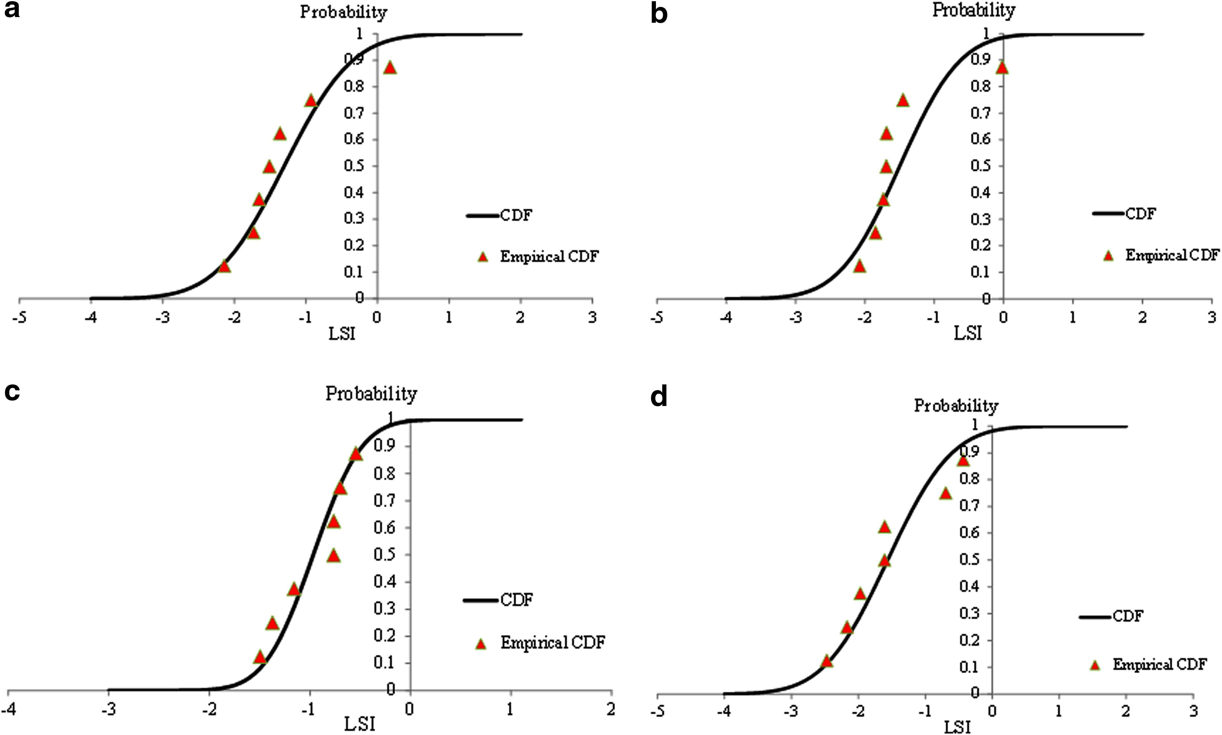
Cumulative distribution function (CDF) curves (black lines) and empirical CDF values (red triangles) of Langelier saturation index (LSI) for (a) RM 46, (b) RM 71, (c) MWW-2, and (d) MWW-3. Empirical CDF values were calculated by Weibull formula, F(i)=rank (i)/(n+1) (Prakash, 2004).

Table 5.

Model-Derived Mean and Standard Deviation of Langelier Saturation Index

Sample	μ (LSI)	σ (LSI)
RM 46	−1.31	0.75
RM 71	−1.50	0.69
MWW-2	−0.97	0.38
MWW-3	−1.56	0.75

Aggressive index

Similar to LSI, AI follows normal distribution, given the assumption that pH, log[Alk], and log[Ca²⁺+Mg²⁺] follow a normal distribution. The mean and variance of AI can be expressed as follows: \documentclass{aastex}\usepackage{amsbsy}\usepackage{amsfonts}\usepackage{amssymb}\usepackage{bm}\usepackage{mathrsfs}\usepackage{pifont}\usepackage{stmaryrd}\usepackage{textcomp}\usepackage{portland, xspace}\usepackage{amsmath, amsxtra}\pagestyle{empty}\DeclareMathSizes{10}{9}{7}{6}\begin{document} \begin{align*}\mu_{{ \rm AI}} = \mu_{{ \rm pH}} + \mu_{{ \rm Log} ( [ { \rm Ca ^{2 +} } ] + [ { \rm Mg^{2 +} } ] ) } + \mu_{{ \rm Log [ Alk ] }} \tag{11}\end{align*} \end{document} \documentclass{aastex}\usepackage{amsbsy}\usepackage{amsfonts}\usepackage{amssymb}\usepackage{bm}\usepackage{mathrsfs}\usepackage{pifont}\usepackage{stmaryrd}\usepackage{textcomp}\usepackage{portland, xspace}\usepackage{amsmath, amsxtra}\pagestyle{empty}\DeclareMathSizes{10}{9}{7}{6}\begin{document} \begin{align*} \sigma_{AI}^2 = & \sigma_{pH}^2 + \sigma_{Log ( [ Ca^{2 + } ] + [ Mg^{2 + } ] ) }^2 \\ & + \sigma_{Log [ Alk ] }^2 + 2 \rho_{pH , \ Log ( [ Ca^{2 + } ]} \\ & {+ _{[ Mg^{2 + } ] ) }} \sigma_{pH} \sigma_{Log ( [ Ca^{2 + } ] + [ Mg^{2 + } ] ) } \\ & + 2 \rho_{pH , Log [ Alk ] } \sigma_{pH} \sigma_{Log ( [ Alk ] ) } \\ & + 2 \rho_{Log ( [ Ca^{2 + } ] + [ Mg^{2 + } ] ) , \ Log [ Alk ] } \sigma_{Log ( [ Ca^{2 + } ]} \\ & {+ _{[ Mg^{2 + } ] ) }} \sigma_{Log [ Alk ] } \tag{12} \end{align*} \end{document}

Based on Equations (11) and (12) and the values in Tables 2 –4, the mean and standard deviation values of AI of river waters and wastewaters are obtained. All results are summarized in Table 6. The resulting normal CDF of AI derived in this manner for each of the sampling locations is compared with the corresponding empirical CDF of the seven observations in Fig. 4, demonstrating the internal consistency of the statistical model for AI.

FIG. 4.

CDF curves (black lines) and empirical CDF values (red triangles) of AI for (a) RM 46, (b) RM 71, (c) MWW-2, and (d) MWW-3. Empirical CDF values were calculated by Weibull formula, F(i)=rank (i)/(n+1) (Prakash, 2004).

Table 6.

Model-Derived Mean and Standard Deviation Values of Aggressive Index

Sample	μ (AI)	σ (AI)
RM 46	10.85	0.74
RM 71	10.66	0.70
MWW-2	11.15	0.36
MWW-3	10.55	0.73

Results and Discussion

Sample-specific LSI and AI values

Figure 5 shows the correlation between LSI and AI based on the results in Table 1 (given a temperature of 20°C). It can be seen that most samples had an LSI value <0 and an AI value between 10 and 12, which represents no scaling formation and moderate corrosion potential. It can also be seen that there is a good linear correlation between LSI and AI (AI=LSI+12, given a temperature of 20°C) from the collected water sample data, which shows the consistency between the theoretical derivation [Eq. (8)] and the negative correspondence between LSI and AI in the observed water samples. This correlation between AI and LSI also makes sense from the perspective of corrosion inhibition. To be specific, a higher LSI means more formation of scales and the formation of protective scales is helpful for corrosion inhibition.

FIG. 5.

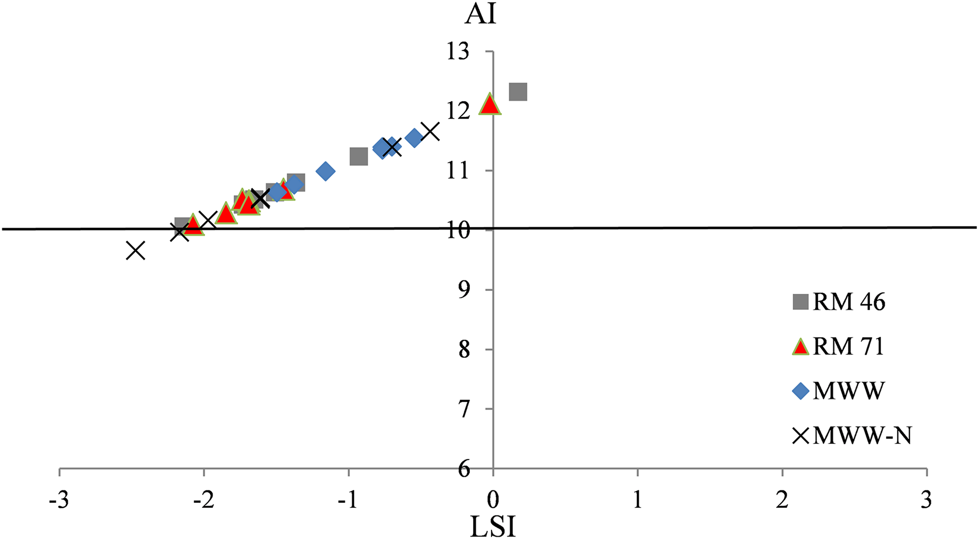
Correlation between aggressive index (AI) and LSI based on values in Table 1.

CDF curves of LSI derived from Equations (9) and (10)

Figure 3a–d shows CDF curves and the empirical CDF values of seven measurements of LSI for two river waters (RM 46 and RM 71) and secondary-treated wastewater and tertiary-treated wastewater, respectively. A good fit of the normal CDF with the empirical CDF indicates that the LSI is normally distributed, and the probability of scaling derived from normal distribution is valid. A poor fit of the normal CDF with the empirical CDF indicates that the LSI is not normally distributed, and the probability of scaling derived from normal distribution is not valid. The goodness-of-fit between normal CDF and empirical CDF of four types of water was calculated by plotting normal CDF values against empirical CDF values, and the correlation coefficients (R²) of the plots were calculated. The plots and the R² values can be found in Supplementary Data (Supplementary Fig. S1). If the R² is high, then the LSI is normally distributed. The empirical CDF values of river water RM 46, secondary-treated wastewater, and tertiary-treated wastewater were consistent with the CDF curves derived from normal distribution (with R² values≥0.9), which demonstrates that the normal distribution can describe the probabilistic distribution of LSI data collected from these waters. The empirical CDF values of river water RM 71 were not as consistent with the CDF curves derived from the normal distribution (R²=0.74), but are still within a moderate level of agreement.

CDF curves of AI derived from Equations (11) and (12)

Figure 4a–d shows CDF curves and the empirical CDF values of seven measurements of AI for two river waters (RM 46 and RM 71), secondary-treated wastewater, and tertiary-treated wastewater, respectively. The empirical CDF values of river water RM 46, secondary-treated wastewater, and tertiary-treated wastewater were consistent with the CDF curves derived from normal distribution, which demonstrates that normal distribution can describe the probabilistic distribution of AI data collected from these waters (see Supplementary Fig. S2 in Supplementary Data for details). The empirical CDF values of river water RM 71 were not fully consistent with the CDF curves derived from the normal distribution, but the inconsistencies still lay within an acceptable range.

Implication and sensitivity analysis

Table 7 summarizes the scaling and corrosion potentials of all four waters tested, as represented by the probabilities that LSI and AI fall within the indicated ranges, as computed from their fitted normal distributions. It can be seen that all the waters tested exhibit a very low probability of forming scale, which is partially due to the mildly acidic nature of the source waters (all waters have an average pH <7). Though the low chance to form scale is good from the perspective of minimizing clogging in cooling water systems, no scale formation can increase the potential for corrosion in pipelines due to the absence of protective scale layers. The corrosion potential results demonstrate that all the waters tested have a high chance to cause moderate corrosion and, for tertiary-treated wastewater, there is moderate chance (∼23%) for the water to cause severe corrosion. In summary, all the four types of water tested have a very low chance to form scales and these waters are suitable for cooling water make-ups from the perspective of scaling minimization. However, the results indicate that additional corrosion-control procedures should be applied when using these waters as cooling water, so as to minimize the possible potential for corrosion in the cooling water system.

Table 7.

Scaling and Corrosion Potentials for Using Indicated River Water, and Secondary- and Tertiary-Treated Wastewaters as Cooling Water Make-Up

	Scaling potential (% probability)		Corrosion potential (% probability)
Sample	Form scale (LSI>0)	No scale (LSI<0)	Severe (AI<10)	Moderate (10<AI<12)	No corrosion (AI>12)
RM 46	4.03	95.97	12.54	81.46	6.00
RM 71	1.49	98.51	17.29	79.93	2.78
MWW-2	0.53	99.47	0.07	99.02	0.91
MWW-3	1.88	98.12	22.56	75.09	2.35

The potentials are represented by probability values computed from the normal distributions for LSI (Table 5) and AI (Table 6).

To assess the sensitivity of LSI and AI to changes in source water quality (in particular, changes in source water pH and temperature), new CDF curves of LSI and AI were derived using the statistical model for each source water. For pH, the sensitivity is evaluated by increasing or decreasing the mean pH by 0.3 units (scenario I: μ(pH)=μ(pH)_original−0.3; scenario II: μ(pH)=μ(pH)_original+0.3). A pH variation of±0.3 is chosen because this variation lies in the range of natural pH variation due to photosynthesis, precipitation, and so on (Department of Ecology at State of Washington, 1991). For temperature, two more cases with temperatures of 10°C and 30°C were evaluated. All new CDF curves for RM 46, RM 71, MWW-2, and MWW-3 are presented in Figs. 6 –8. It can be seen that the LSIs of both river water and MWW were not sensitive to these small pH changes (±0.3) at the threshold value (LSI=0). However, the AIs of both river water and tertiary-treated wastewater were sensitive to the 0.3-unit pH changes at the threshold value (AI=10) and only the AI of secondary-treated wastewater was not sensitive to the pH change considered. As a result, if river water and tertiary-treated wastewater are used as cooling water, a small change in pH may result in a significant change in corrosion potential. As to temperature change, due to acidic nature of all waters tested (the average pHs of all waters were slightly below seven), the temperature change did not cause a significant change in scaling potential. However, if the waters tested had a high average pH, then the temperature increase would result in a significant increase in scaling potential.

FIG. 6.

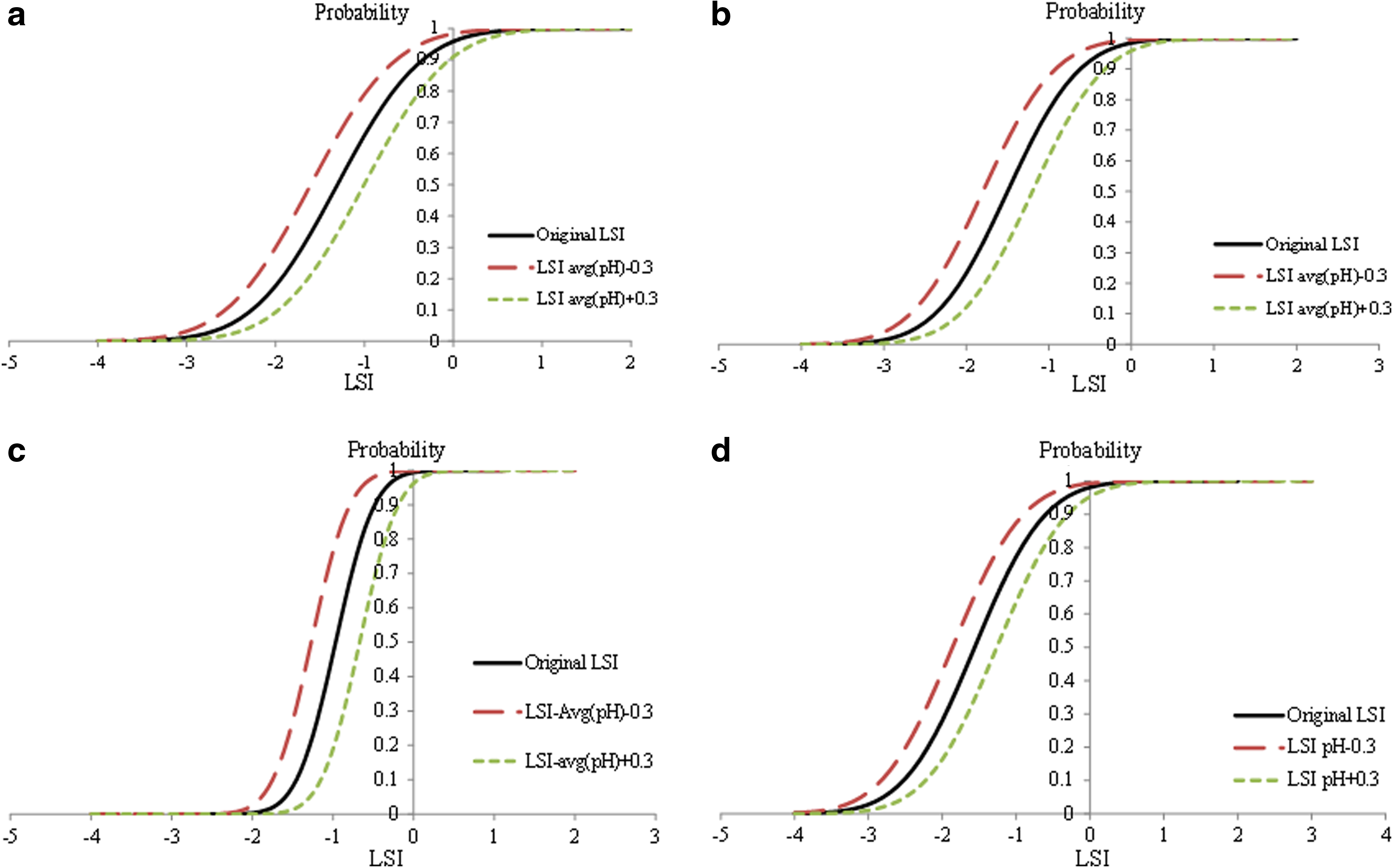
Sensitivity of the CDF curves of LSI to pH change. Three scenarios were tested: (1) original; (2) μ(pH)−0.3; and (3) μ(pH)+0.3. (a) RM 46, (b) RM 71, (c) MWW-2, and (d) MWW-3.

FIG. 7.

Sensitivity of the CDF curves of LSI to temperature change. Three scenarios were tested: (1) original (T=20°C); (2) low-temperature scenario (T=10°C); and (3) high-temperature scenario (T=30°C). (a) RM 46, (b) RM 71, (c) MWW-2, and (d) MWW-3.

FIG. 8.

Sensitivity of the CDF curves of AI to pH change. Three scenarios were tested: (1) original; (2) μ(pH)−0.3; and (3) μ(pH)+0.3. (a) RM 46, (b) RM 71, (c) MWW-2, and (d) MWW-3.

In summary, the results from the case study show that the slightly acidic nature of the water samples collected makes corrosion the main concern if water from the four sampling locations is used as cooling water. From the initial data evaluated in this study, secondary-treated MWW collected from FTMSA, Pennsylvania (MWW-2) might be a better candidate as a cooling water alternative from the perspective of scaling and corrosion minimization compared with other three types of water tested. However, this study does not take into account the high content of organic matter, phosphate, and ammonia in secondary-treated MWW, which could increase the potential for biofouling in the cooling system (Hsieh et al., 2010). As a result, if secondary-treated MWW is used as cooling water, biofouling inhibitors are generally required to prevent the growth of biomass in the cooling system, though biofouling inhibitors can have very adverse effects when discharged to watercourses.

This study classifies four types of water that have different potentials to cause scaling and corrosion (Fig. 9). Type I water has a low chance to cause scaling and a moderate chance to cause corrosion. This type of water has an average LSI value of around −1 and a relatively low standard deviation of LSI (σ [LSI]<1). Type II water has a high chance to cause scaling and low chance to cause corrosion. This type of water has an average LSI value around 1 and a low-to-moderate standard deviation of LSI. Type III water has a high chance of causing corrosion and a low chance of causing scaling. This type of water has an average LSI value of around −3 and a low-to-moderate standard deviation of LSI. Type IV water has the potential to cause both corrosion and scaling. This type of water has a high standard deviation of LSI; thus, it is possible for the LSI to be in the range that causes scaling in some samples, with the AI in the range associated with corrosion for other samples.

FIG. 9.

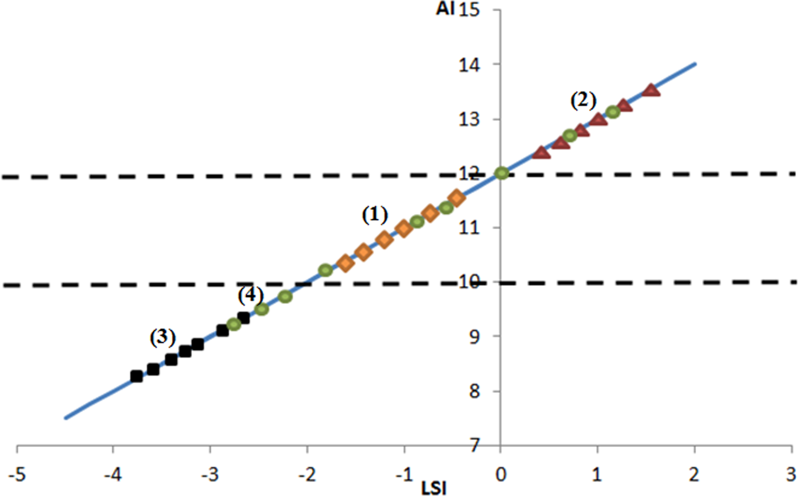
Classification of four types of water that have different potentials for scaling and corrosion. (1)=Type I water (orange diamonds); (2)=type II water (red triangles); (3)=type III water (black squares); and (4)=type IV water (green circles).

Conclusions

A statistical model for variations in the LSI and AI across multiple samples of a water source was developed to characterize the potential of freshwater and treated wastewater to be used in the thermoelectric power plant cooling system as an alternative source of cooling water. The statistical model was found to provide a good representation of sample-to-sample variations in LSI and AI resulting from fitted distributions for their contributing parameters (pH, Alk, Mg²⁺ and Ca²⁺). Using the basic water quality parameters to compute the scaling and corrosion indices, the statistical analysis results showed that samples of freshwater, secondary-treated MWW, and tertiary-treated MWW collected in this study have a very low probability of forming scales in the cooling system, whereas all the waters have a relatively high probability of being moderately corrosive to the cooling system. Compared with freshwater and tertiary-treated wastewater, secondary-treated wastewater has a lower probability to be very corrosive (AI<10). Therefore, an anticorrosive agent (e.g., tolytriazole or zinc and phosphate containing chemicals) may be added to reduce the corrosion potential when using these waters as cooling water make-ups. However, the amount of anticorrosive agent added needs to be carefully controlled, because the anticorrosive agents are hard to degrade, and they may enter rivers and groundwater via wastewater discharge. Considering both LSI and AI results for the samples analyzed, the secondary-treated wastewater is the best candidate to be used as cooling water make-up (so long as the potential for biofouling is addressed).

Footnotes

Acknowledgments

The authors of this article would like to thank FTMSA, Murrysville, Pennsylvania, for the treated wastewater samples. We appreciate helps from Jessica Wilson, Yuxin Wang, Juan Peng, and Ronald Ripper at Department of CEE, Carnegie Mellon University for freshwater sampling and laboratory work. The authors would also like to thank David Dzombak at Department of CEE, Carnegie Mellon University and Radisav Vidic at Department of CEE, University of Pittsburgh for their invaluable comments on this article.

Author Disclosure Statement

No competing financial interests exist.

References

Ahmad

(2006). Principles of Corrosion Engineering and Corrosion Control (1st edition). Oxford: Butterworth-Heinemann.

Assembly of Life Sciences (U.S.) (1982). Drinking Water and Health (Vol.4). Washington, DC: National Academies Press.

Bjerg

P.L.

, and Christensen

T.H.

(1992). Spatial and temporal small-scale variation in groundwater quality of a shallow sandy aquifer. J. Hydrol., 131, 133.

Buyuksagis

, and Erol

(2012). The examination of afyonkarahisar's geothermal system corrosion. J. Mater. Eng. Perform., 22, 563.

Cheremisinoff

N.P.

, and Cheremisinoff

P.N.

(1981). Cooling Towers Selection, Design and Practice. Ann Arbor, MI: Ann Arbor Science Publishers, Inc.

Chien

C.C.

, Kao

C.M.

, Chen

C.W.

, Dong

C.D.

, and Chien

H.Y.

(2009). Evaluation of biological stability and corrosion potential in drinking water distribution systems: A case study. Environ. Monitor. Assess., 153, 127.

Chien

S.H.

, Hsieh

M.K.

, Li

, Monnell

, Dzombak

D.A.

, and Vidic

(2012). Pilot-scale cooling tower to evaluate corrosion, scaling, and biofouling control strategies for cooling system makeup water. Rev. Sci. Instrum., 83, 1.

Cloete

T.E.

, Jacobs

, and Brözel

V.S.

(1998). The chemical control of biofouling in industrial water systems. Biodegradation., 9, 23.

Department of Ecology at State of Washington. (1991). A Citizen's Guide to Understanding and Monitoring Lakes and Streams, Chapter 3: Streams. Available at: www.ecy.wa.gov/programs/wq/plants/management/joysmanual/streamph.html (accessed June 16, 2014).

10.

Eaton

A.D.

, Clesceri

L.S.

, Rice

E.W.

, and Greenberg

A.B.

(editors) (2005). The Standard Methods for Examination of Water and Wastewater. Washington, DC: American Public Health Association.

11.

Ehrhardt

R.F.

, Tucker

R.C.

, and Fabian

T.R.

(1986). Analysis of Alternative Sources of Cooling Water (EPRI-EA-4732). Palo Alto, CA: Electrical Power Research Institute.

12.

French Creek Software, Inc. (1999). WaterCycle Rx: Predictive Modeling of Scale, Corrosion, & Inhibitor Dosages for Cooling Waters. Available at: www.frenchcreeksoftware.com/wcmanual.pdf (accessed October 23, 2013).

13.

Gupta

, Nafees

S.M.

, Jain

M.K.

, and Kalpana

(2011). Assessment of groundwater quality of outer skirts of Kota City with reference to its potential of scale formation and corrosivity. E. J. Chem., 8, 1330.

14.

Hach , (2009). Langelier and Aggressive Indices. Method 8073. Available at: www.hach.com/asset-get.download-en.jsa?id=7639984187 (accessed April 15, 2014).

15.

Hsieh

M.K.

, Li

, Chien

S.H.

, Monnell

J.D.

, Choudhury

, Dzombak

D.A.

, and Vidic

R.D.

(2010). Corrosion control when using secondary treated municipal wastewater as alternative makeup water for cooling tower systems. Water Environ. Res., 82, 2346.

16.

Kenny

J.F.

, Barber

N.L.

, Hutson

S.S.

, Linsey

K.S.

, Lovelace

J.K.

, and Maupin

M.A.

(2009). Estimated Use of Water in the United States in 2005. Circular No.1344, 52. A circular by U.S. Geological Survey, Reston.

17.

Kinsela

A.S.

, Jones

A.M.

, Collins

R.N.

, and Waite

T.D.

(2012). The impacts of low-cost treatment options upon scale formation potential in remote communities reliant on hard groundwaters. A case study: Northern Territory, Australia. Sci. Total Environ., 416, 22.

18.

Langelier

W.F.

(1936). The analytical control of anticorrosion water treatment. J. Am. Water Works Ass., 28, 1500.

19.

, Chien

, Hsieh

M.K.

, Dzombak

D.A.

, and Vidic

R.D.

(2011). Escalating Water Demand for Energy Production and the Potential for Use of Treated Municipal Wastewater. Environ. Sci. Technol., 45, 4195.

20.

Liu

, Chien

, Dzombak

D.A.

, and Vidic

R.D.

(2012). Mineral scaling mitigation in cooling systems using tertiary-treated municipal wastewater. Water Res., 46, 4488.

21.

Luo

, Zhao

, Liang

, and Dong

(2009). Study on water quality chemical stability of desalinated seawater in municipal water supply systems. Environ. Sci. Info. App. Technol., 1, 344.

22.

Meesters

K.P.H.

, Van Groenestijn

J.W.

, and Gerritse

(2003). Biofouling reduction in recirculating cooling systems through biofiltration of process water. Water Res., 37, 525.

23.

Macknick

(2012). Water Impacts of the Electricity Sector. National Renewable Energy Laboratory, Golden, CO. Available at: www.nrel.gov/docs/fy12osti/55028.pdf (accessed April 15, 2014).

24.

Ott

(1990). A physical explanation of the lognormality of pollutant concentrations. J. Air Waste Ma., 40, 1378.

25.

Prakash

(2004). Water Resource Engineering: Handbook of Essential Methods and Design. Reston: ASCE Publications.

26.

Rafferty

(1999). Scaling in geothermal heat pump systems. Prepared for: U.S. Department of Energy, Idaho Operations Office, and 785 DOE Place, Idaho Falls, ID 83401. Contract No. DE-FG07-90ID 13040.

27.

Sheikh

A.K.

, Zubair

S.M.

, Younas

, and Budair

M.O.

(2001). Statistical aspects of fouling processes. P. I. Mech. Eng. E-J. Pro., 215, 331.

28.

Small

M.J.

, Sutton

M.C.

, and Milke

M.W.

(1988). Parametric distributions of regional lake chemistry: Fitted and derived. Environ. Sci. Technol., 22, 196.

29.

Swart

J.S.

, and Engelbrecht

J. P.

(2004). Pilot scale evaluation of mine water (MW) as a cooling medium. Water SA. 40, 145.

30.

Taghipour

, Shakerkhatibi

, Pourakbar

, and Belvasi

(2012). Corrosion and Scaling Potential in Drinking Water Distribution System of Tabriz, Northwestern Iran. Health Promot., 2, 103.

31.

U.S. EPA, (2009). Drinking Water Glossary: A Dictionary of Technical and Legal Terms Related to Drinking Water. Washington, DC: Office of Water/Office of Ground Water and Drinking Water.

32.

U.S. EPA, (2010). Proposed Information Collection Request for a General Population Survey to Allow the Estimation of Benefits for the Clean Water Act Section 316(b) Cooling Water Intake Structures Rulemaking. U.S. Environmental Protection Agency, Office of Water. Available at: www.epa.gov/waterscience/316b/ph2.htm (accessed April 15, 2014).

33.

U.S. EPA, (2014). Power Plants in the Mid-Atlantic Region. Available at: www.epa.gov/reg3artd/globclimate/r3pplants.html (accessed June 11, 2014).

34.

Vidic

R.D.

, and Dzombak

D.A.

(2009). Reuse of Treated Internal or External Wastewaters in the Cooling Systems of Coal Based Thermoelectric Power Plants. Final Technical Report submitted to U.S. Pittsburgh, PA: Department of Energy, National Energy Technology Laboratory.

35.

Zdaniuk

G.J.

, Chamra

L.M.

, and Mago

P.J.

(2006). A literature survey of water-side fouling applicable to cooling tower condensers. P. I. Mech. Eng. A-J. Power Energy., 815, 27.

36.

Zuane

J.D.

(1997). Handbook of Drinking Water Quality. New York, NY: John Wiley and Sons.

Supplementary Material

Please find the following supplemental material available below.

For Open Access articles published under a Creative Commons License, all supplemental material carries the same license as the article it is associated with.

For non-Open Access articles published, all supplemental material carries a non-exclusive license, and permission requests for re-use of supplemental material or any part of supplemental material shall be sent directly to the copyright owner as specified in the copyright notice associated with the article.

0.00 MB

0.62 MB