Fate of Surface Spills of Cold Lake Blend Diluted Bitumen Treated with Dispersant and Mineral Fines in a Wave Tank

Oil, dispersant, and MF application

CLB, obtained from industry (Canmet Energy), was selected because it represents the highest volume of dilbit products transported by pipeline in Canada. Similar to the technique used by Li et al. (2009a), the CLB dilbit product was artificially weathered by purging it with nitrogen for 48 h at ∼20°C. The mass of the product was recorded before and after weathering. Measured physical and chemical properties for CLB and other oil products can be obtained in a report by the Government of Canada (2013).

The experimental and sampling procedures were consistent with the crude oil dispersant efficacy testing in the flow-through wave tank reported previously (Li et al., 2008, 2009a, 2009c). Briefly, for each experiment, ∼240 g of dilbit was gently poured onto the filtered seawater surface within a 40-cm diameter ring located 1,000 cm downstream from the wave maker, and ∼12 g of dispersant was sprayed gently onto the oil slick through a pressurized nozzle (60 psi, 0.635 mm i.d.). This resulted in a dispersant-to-oil ratio of 1:20 (Li et al., 2008, 2009a, 2009c, 2010). In some experiments, MF were used in combination with dispersant application as an additional treatment option. The MF were Kaolin (kaolinite clay mineral particle sizes ranging from 0.1 to 4 μm; Sigma Aldrich) prepared as a seawater slurry at a concentration of 50 g/L. The slurry (at a 1.5:1 ratio to oil) was applied by a hand operated sprayer, which provided a uniform distribution of MF over the oil surface and minimized disruption of oil on the water surface. Then, the wave maker was started, and the ring was then promptly lifted before the arrival of the first wave breaker on the location of the ring. The sequence of waves aimed at generating a breaker every 40 s at the same location (where the ring was placed earlier) using the dispersive focusing technique (Botrus et al., 2008). A plunging breaker (where the water reenters the water surface downstream) was generated with a height of 40 cm, as our earlier findings (Government of Canada, 2013) revealed that spill treating agents were ineffective when no wave breaking occurred. Each experiment was conducted for 1 h during which each wave cycle (four breakers) lasts for 15 s, followed by a quiescence period that lasts for 25 s. Therefore, there are four breaking waves every 40 s in the test tank, producing a total of 360 breakers during a 1-h oil spill experiment.

Wave tank in situ measuring devices

Two particle size counters (LISST-100X; Sequoia Scientific, Inc.) were employed during the experiments at 120 cm and 1,100 cm downstream of the oil release point and at a depth of 45 cm (Fig. 1). Particle size distributions were recorded at 2.0–5.0 s intervals for 1 h per experiment (Li et al., 2008, 2009a, 2009c, 2010).

Laboratory analysis of seawater samples

Four water sampling devices were deployed, one at 200 cm upstream from the oil release point and the other three downstream at 200, 800, and 1,200 cm from the oil release point (Fig. 1). Each of the four samplers collected water (∼100 mL) at three depths (5, 75, and 140 cm) in the tank at the time points 5, 15, 30, 45, and 60 min. In addition, surface samples ∼500 mL were taken from near location D (Fig. 1) and effluent samples (from the side opposite the wave maker) were taken. Time zero samples (before oil release, to check background levels) were selected arbitrarily at 1,200 cm downstream (location D in Fig. 1) throughout the study. The factorial design in Table 1 was conducted in random order to reduce systematic errors from confounding effects from wind, rain, seawater salinity, and temperature.

Subsamples (20 mL) of collected water samples were used to measure the dispersed oil–water interfacial tension in a temperature controlled environment (20.1°C±0.3°C) using the Wilhelmy plate method (Drelich et al., 2002; King et al., 2013). The remainder of the water samples were extracted and analyzed for total petroleum hydrocarbons (TPHs) using a gas chromatograph equipped with flame ionization detection (GC-FID) according to the method of Cole et al. (2007). The method is a modified version of EPA 3500C whereby the sample container is the extraction vessel. Briefly, 12 mL of dichloromethane (DCM) was added to a 125-mL amber glass sample bottle containing ∼80 mL of seawater collected during the experiments. Next, the sample was placed on a Wheaton R₂P roller (VWR) for 18 h. The roller has been modified to accommodate a 3-inch (i.d.) PVC pipe into each roller slot. This modification permits sample containers of different sizes to be used in the apparatus. Once extraction was complete, the sample bottles were removed and the DCM was recovered. The recovered DCM was placed in a preweighed 15-mL centrifuge tube, and the solvent was removed using a nitrogen evaporator until the final volume reached 1.0 mL graduation on the centrifuge tube. The extracts were then analyzed by GC-FID. Calibration standards based on CLB dilbit were used to develop calibration curves for evaluating the oil concentration in the seawater extracts. A mean percent recovery of 90.8%±4.6% was calculated from all oils spiked into seawater. The method detection limit is <0.5 mg/L. The benefit of this procedure is that 240 samples can be extracted simultaneously by one person (depending on the number of rollers used), thus increasing productivity with acceptable accuracy and precision (Supplementary Data). Extracts of seawater surface samples were evaluated for TPHs. The results for these supporting tests are presented as Supplementary Data.

Synthetically weathered dilbit products

The CLB lost 6.2% of its mass, which is consistent with the natural weathering study conducted by King et al. (2014), in the wave tank under quiescent conditions. Preweathered oils were used to reflect the fact that spilled oil will begin to weather once it is released, and most of the weathering of oil spilled on the water surface occurs due to evaporation in 24–48 h following a spill (Fingas, 1999). Since response time to treat a spill can take up to 24 h, it is critical that our studies take into consideration that any treatment of spills at sea would be applied to weathered oil.

Physical measurements in the wave tank

To capture seasonal effects on a CLB dilbit spill, experiments were conducted in the spring and summer of 2013, and the physical measurements obtained are recorded in Table 1. During the spring experiments, the water temperature in the tank was 8.5°C±1.3°C. During the summer experiments, it was 17.0°C±2.6°C. The proposed Enbridge Northern Gateway pipeline will transport dilbit products from Bruderheim, Alberta, to the Port of Kitimat, British Columbia, on the western coast of Canada. The seasonal temperatures reported here are coincidently consistent with seasonal water temperatures on the western coast of Canada (Stronach et al., 2010). Water temperature is an important factor to consider since it can affect the effectiveness of oil spill treatments applied to conventional oils (Li et al., 2010).

Note that in Kitimat and the Douglas Channel, British Columbia, Canada, water salinities vary from less than 20 to 33 practical salinity units (psu), depending on sea location and depth (ASL Environmental Sciences, Inc., 2010). Salinity is also an important factor to consider since it can affect the efficacy of oil spill treatments applied to conventional oils (Chandrasekar et al., 2006). In that study, they tested the effects of salinity in the range of 10–34 psu on the chemical dispersion of crude oils and determined that oil dispersion increased with increasing salinity. The average salinity was 28 psu during the spring experiments and 27 psu during the summer experiments. The small difference between these values suggests that salinity variation would not make a measureable impact on the behavior of oil during the experiments. It is important to note, in Table 1, the lowest salinity value recorded was 21.0 psu when dispersant was applied to CLB during the summer experiments. However, for all three CLB trials conducted with this treatment, the dispersion effectiveness was similar even though the water salinity ranged from 21.0 to 28.1 psu.

In situ LISST

Previous wave tank studies have shown that floating oil that becomes dispersed and driven into the water column under breaking waves in the presence of chemical dispersant has oil droplet sizes in the range of 2.5–70 μm in a distinctive, bimodal or multimodal droplet size distribution (DSD) (Li et al., 2009b). These oil droplets remain dispersed and do not coalesce. However, oil droplets that have been produced by breaking waves in the absence of dispersant are typically larger than 70 μm, have a unimodal distribution, and tend to ascend and coalesce at the surface. Thus, the use of the LISST particle size analyzer (upper particle size limit of 500 μm) is suitable for differentiating between chemically enhanced and naturally dispersed oil.

Figure 2 reports the concentration of droplets obtained in spring from LISST#1 (120 cm from the oil application location, Fig. 1) during each of the experimental conditions. Each graph also reports, in the legend, the total particle concentration (TPC) and the volume mean diameter (VMD). Without any treatment, the CLB showed poor natural dispersion where very little oil (in dispersed form) was in the water column; at or near the largest size (i.e., 500 μm), the droplets had a non-negligible concentration, but still small. The addition of MF resulted in a larger concentration at or near the largest particle size (i.e., 500 μm), reflecting ineffective dispersion. The increase in the small diameter (2–30 μm) might not be due to oil, but to the added MF whose sizes were less than 5 μm. The dispersant alone appears to slightly increase the concentration around 35 μm, which has to be an increase in oil concentration as the sizes of the MF were less than 5 μm. The case of dispersant+MF provided a broad DSD from the LISST accompanied by the largest concentration values; one notes (Fig. 2) a gradual increase from 10 until 60 μm, thus leveling off and decreasing as the maximum is approached. The oil DSD was broadest for the dispersant+MF, followed by the cases with dispersant, which seem to be comparable.

OPEN IN VIEWER

FIG. 2.

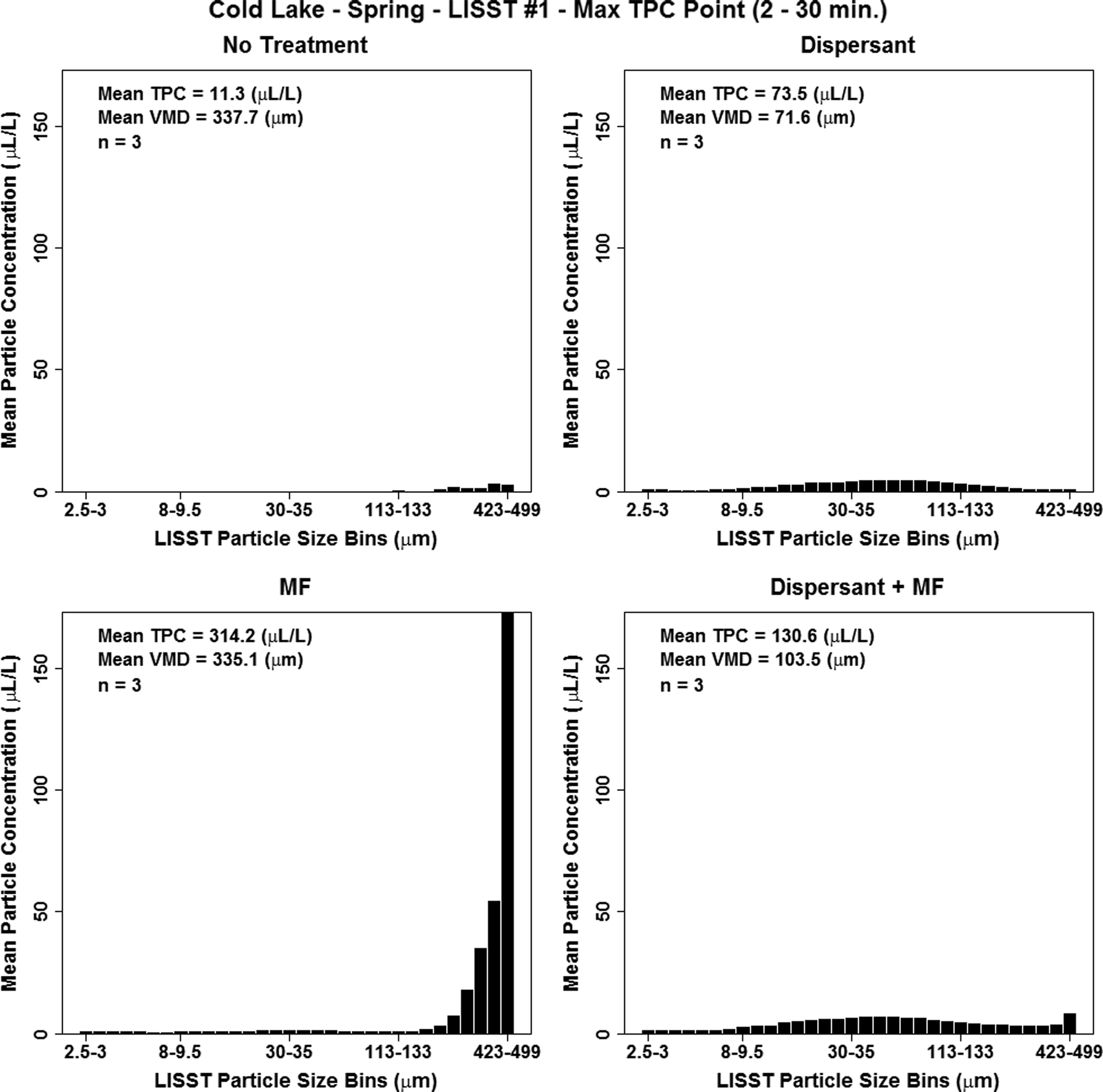
Spring data for Cold Lake Blend (CLB) dilbit obtained from LISST#1 (120 cm from oil release). Each plot is an average of triplicate experiments using the particle size distribution data obtained at the time point of maximum total particle concentration (TPC) within the first 30 min of the experiment. The graph (with mineral fines [MF]) contains data from only two replicates due to an instrument malfunction. X-axis values represent the 32 logarithmically spaced particle size bins generated by the LISST100X instrument. VMD, volume mean diameter.

The VMD for CLB with no treatment and MF was ∼340 μm, much larger than the VMD of other systems. The high concentrations for MF and dispersant+MF can be also inferred from the large TPC values of 314 and 130 μL/L, respectively, and in comparison, the other systems are <75 μL/L. The VMD of <75 μm was the lowest when dispersant was present. The case with dispersant+MF only provided a VMD at ∼104 μm.

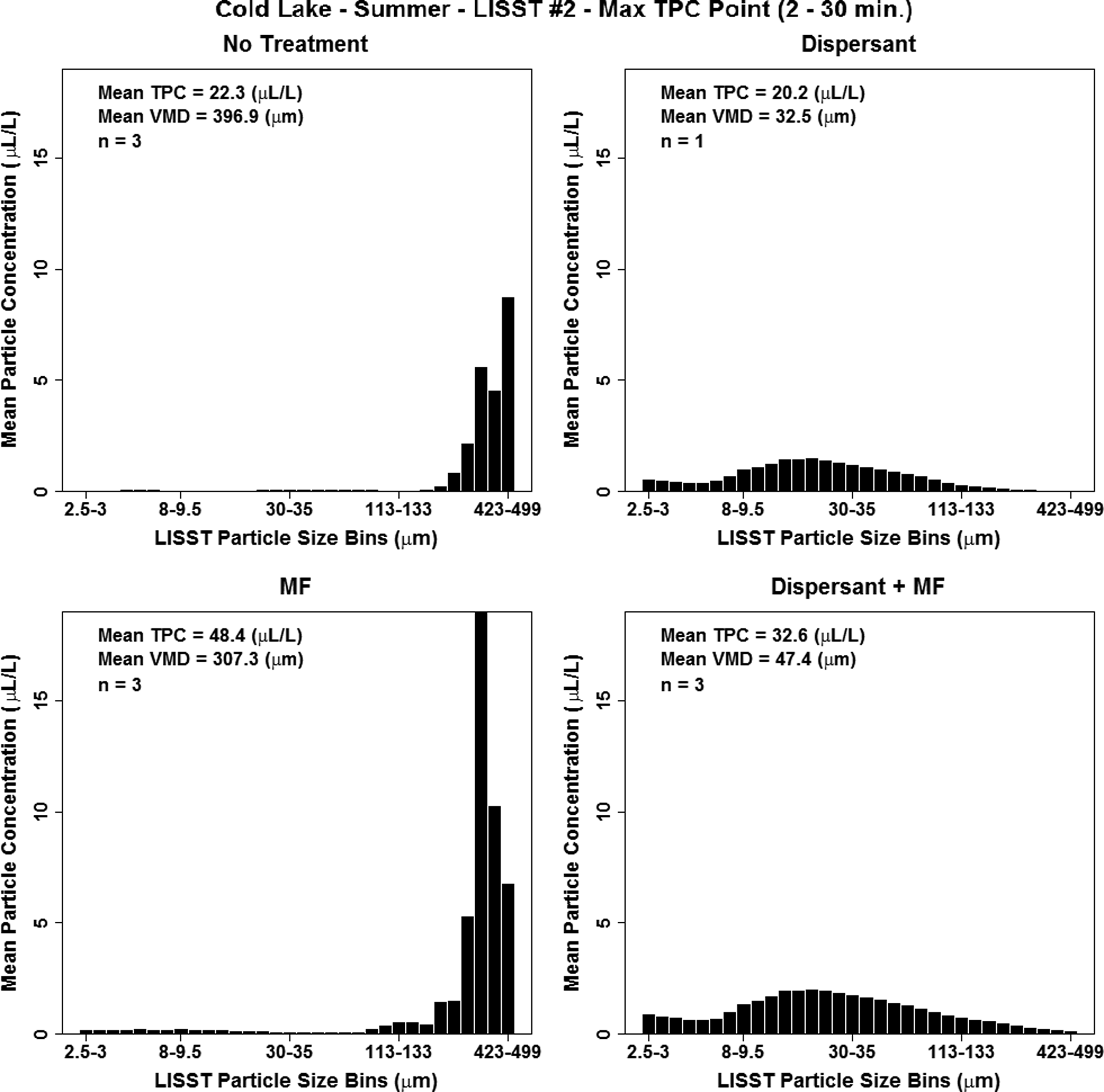
Figure 3 shows the particle size distribution for the same cases reported in Figure 2, but for summer conditions. Similar trends, as reported in Figure 2, were evident where the no treatment and MF showed poor natural dispersion with only the largest size (i.e., 500 μm) particles displayed; however, MF treatment also displayed smaller size particles at negligible amounts. The dispersant alone and dispersant+MF appear to slightly increase the concentration from 10 to 20 μm, followed by a decline near 20. The large particles (Fig. 3) produced indicate that some of the oil was not effectively dispersed and thus the present of large (>70 μm) oil droplets. LISST data using MF are difficult to interpret since the LISST is unable to differentiate between small particles of sediment, oil-particle aggregates, and droplets of oil. However, the data shown in the lower panels of Figures 2 and 3 suggest that the number of oil droplets due to dispersant+MF is much larger than that due to MF alone (bottom left panels). For no treatment and MF to CLB, the summertime results are slightly higher compared with the same treatments conducted in springtime. However, these differences are considered to be negligible and the difference can be better explained by the chemistry data.

OPEN IN VIEWER

FIG. 3.

Summer data for CLB dilbit obtained from LISST#1 (120 cm from oil release). Each plot is an average of triplicate experiments using the particle size distribution data obtained at the time point of maximum TPC within the first 30 min of the experiment. The graph (with MF) contains data from only two replicates due to an instrument malfunction. X-axis values represent the 32 logarithmically spaced particle size bins generated by the LISST100X instrument.

Figure 4 presents the concentration of droplets obtained in spring from LISST#2 (i.e., at 1,200 cm downstream of the oil release). The VMD values for no treatment and MF follow the same pattern as for LISST#1, and the values for the dispersant cases are comparable with those with dispersant at LISST#1 (Fig. 2). The TPCs in Figure 4 are usually smaller than those at LISST#1 (Fig. 2) most likely due to dilution as the plume traveled 1,000 cm downstream of the wave tank.

OPEN IN VIEWER

FIG. 4.

Spring data for CLB dilbit obtained from LISST#2 (1,100 cm from oil release). Each plot is an average of triplicate experiments using the particle size distribution data obtained at the time point of maximum TPC within the first 20 min of the experiment. X-axis values represent the 32 logarithmically spaced particle size bins generated by the LISST100X instrument.

Figure 5 shows the particle concentration of droplets obtained in summer from LISST#2. The VMD was large (>390 μm) for no treatment. The VMD was 32 μm when dispersant was present compared with 290 μm from LISST#1 (Fig. 3). However, the VMD for the MF only was similar to those obtained from LISST#1 (Fig. 3). The TPCs in Figure 5 are usually smaller than those at LISST#1 (Fig. 2) most likely due to dilution as the plume traveled 1,000 cm downstream of the wave tank. There are obvious differences in particle size distribution when comparing LISST#1 with LISST#2. LISST#1 is located ∼100 cm downstream of the oil release point where initial dispersion of dilbit takes place. LISST#2 is located ∼1,200 cm downstream of oil release where dilution (by way of the flow-through) of the dispersed dilbit is more pronounced.

OPEN IN VIEWER

FIG. 5.

Summer data for CLB dilbit obtained from LISST#2 (1,100 cm from oil release). Each plot is an average of triplicate experiments using the particle size distribution data obtained at the time point of maximum TPC within the first 30 min of the experiment. The graph (with MF) contains data from only two replicates due to an instrument malfunction. X-axis values represent the 32 logarithmically spaced particle size bins generated by the LISST100X instrument.

More evident under summer conditions is the effect of the dispersant treatment to CLB where the concentration of small particles (<70 μm) increased in comparison with other settings; ∼50–60% of the total particles detected were <70 μm, a considerable increase in dispersion over the cases without dispersant. In addition, VMD dropped noticeably to 79 μm (Fig. 5), indicating that the dispersion of the CLB is enhanced by the application of chemical dispersant under summer conditions. Further information on the mean TPCs can be found in Supplementary Data.

In summary, the results of Figures 2–5 suggest that the treatment with dispersant only increased the concentration of oil (TPC) in the form of small (<70 μm) droplets in the water column, but that treatment with dispersant+MF did not result in considerable dispersion. In addition, the resulting dispersion had a particle size unimodal distribution in general (in the size range from 2.5 to 70 μm), which is different than the observed particle size bimodal distribution when conventional oils are treated with dispersant (Li et al., 2009b).

Hydrocarbon analyses

During the spring and summer wave tank experiments, samples at various locations and depths over time were obtained and subsequently analyzed for hydrocarbon concentrations. The mean of three replicates of measurements at three depths at 12 m downstream of oil release and the mean of three replicates of the effluent (at the end of the wave tank) were obtained. They were plotted as a function of time for each of the four cases considered herein for both spring (Fig. 6) and summer (Fig. 7).

OPEN IN VIEWER

FIG. 6.

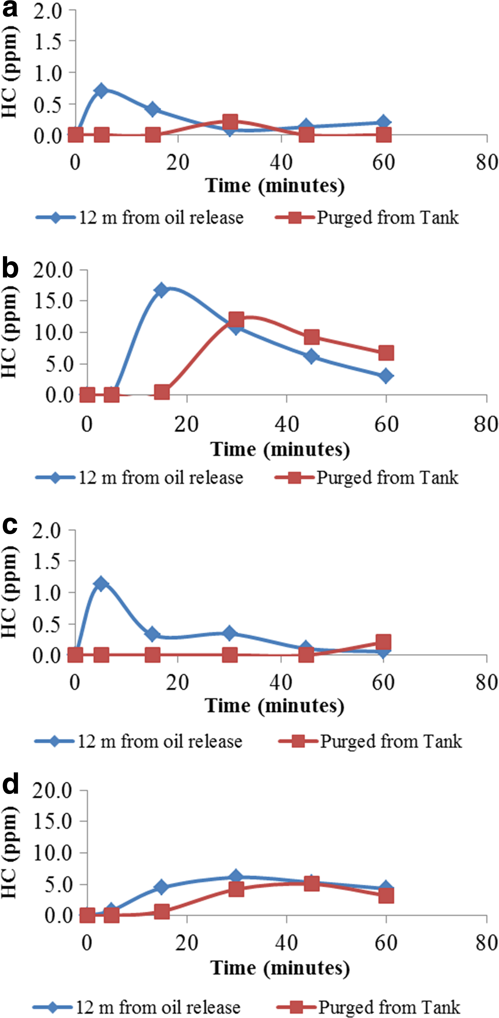
Spring conditions: HC concentrations for the dispersion of CLB under (a) no treatment, (b) dispersant, (c) mineral fines (MF), and (d) dispersant+MF. Note the large vertical scale when dispersant is used (b and d).

OPEN IN VIEWER

FIG. 7.

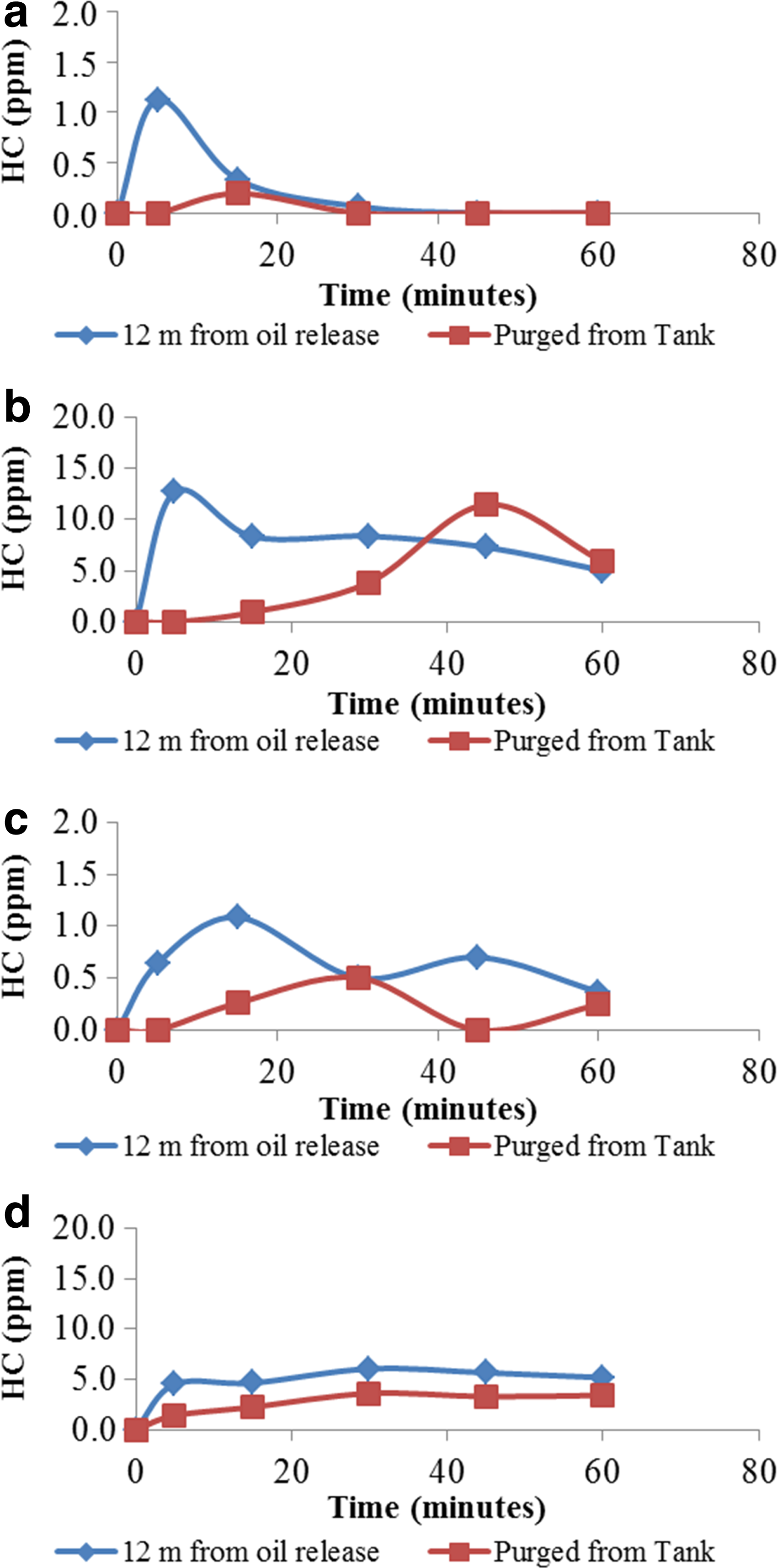
Summer conditions: HC concentrations for the dispersion of CLB under (a) no treatment, (b) dispersant, (c) MF, and (d) dispersant+MF. Note the large vertical scale when dispersant is used (b and d).

Spring results show that under no treatment (Fig. 6a) the TPH concentration at 1,200 cm reached its maximum in ∼5 min, and it was around 0.8 ppm. The effluent concentration (Fig. 6a) increased with time slower than that at 1,200 cm, which is understandable considering that the effluent concentration was obtained from the end of the tank. The concentration in the effluent was more or less uniform and less than the maximum at 1,200 cm, which is most likely due to dilution. When dispersant was used (Fig. 6b), the concentration of the 1,200 cm and effluent remained at the background value for 5 and 15 min, respectively. Then, the concentration increased to >10 ppm. The peak time for the 1,200 cm occurred earlier than that of the effluent by ∼15 min. The fast arrival of the hydrocarbon concentration for the no treatment case in comparison with the dispersant case is probably due to the fact that nondispersed oil remained at the water surface, and thus got advected rapidly downstream by waves, because the water speed due to waves decreases with depth; Boufadel et al. (2006) investigated the advection of oil droplets due to waves and found that droplets with higher buoyancy (e.g., large) advect faster than those with lower buoyancy (smaller droplets). The addition of dispersant probably caused the oil to spread in the water column where the forward advective velocity is small, which caused a delay in the arrival as noted in Figure 6b. However, when the oil plume arrived at the sampling locations, its concentration was much larger than that of the undispersed oil. This justifies some of the concerns regarding chemically dispersed oils and that their concentration in the water column could increase to make them toxic to organisms (Schein et al., 2009; McIntosh et al., 2010).

Figure 6c (CLB treated with MF) shows that the concentration of TPHs in the effluent is similar to that of the effluent from the no treatment case (Fig. 6a). However, the concentration at 1,200 cm shows a rapid rise at 5 min, followed by a decline at 15 min, which levels off and returns to background at 45 min. The broad hydrocarbon distribution over time can be explained based on the fact that oil that adsorbs to the MF tends to sink; therefore, it would move downstream slower than oil with no treatment. The MF treatment produced a higher hydrocarbon value (1.2 ppm) in comparison with the no treatment case (0.8 ppm), but the difference is well within the analytical variance of the method that was used to obtain the results.

Figure 6d is essentially an intermediate between Figure 6b and c. The high values are obviously due to the dispersant. However, the slow rises are probably due to the MF on the oil, which slowed down the leaching rate of soluble oil components into the water column. Thus, when MF are used, it seems that the arrival of the hydrocarbons to the effluent is greatly dependent on the dynamics of the clay mineral. The dispersant, on the other hand, seems to affect mainly the initial concentration of hydrocarbons that enters the water column. In other words, the dispersant seems to affect the fate of the oil (free phase or dissolved), and the MF seem to affect its transport. This highlights some of the advantages of wave tank studies over laboratory flasks (i.e., that it can account for transport).

For the summer data, Figure 7a (no treatment) shows that the TPH concentration (at the 1,200 cm location) increased to 1.2 ppm (it reached 0.8 ppm in spring, Fig. 6a) in ∼5 min. The concentration (at the effluent) remained near background values, except for a slight increase at 15 min. The differences in the spring and summer results are negligible since the hydrocarbon concentrations are approaching the method detection where analytical variance is highest. When dispersant was used (Fig. 7b), the TPH concentration (at 1,200 cm location) increased rapidly to reach values around 15 ppm, while the maximum was greater than 15 ppm in the spring data (Fig. 6b). However, in springtime, the TPH concentrations declined more rapidly compared with summertime results. In springtime, the effluent concentration remained at background values for 15 min, and then increased gradually to reach a maximum around 12 ppm. In summertime, the effluent concentration gradually increased to a maximum around 10 ppm at 45 min.

Figure 7c (MF) shows that the effluent concentration rose at time 5 min and then remained more or less uniform at a concentration of ∼0.5 ppm. This behavior is dissimilar to what we noted for the no treatment case in summer (Fig. 7a) and spring (Fig. 6a) and the MF treatment in spring (Fig. 6c). This would suggest that MF application appears to be more effective in warm waters. At 1,200 cm, the concentration increased rapidly, and then dropped relatively fast (but slower than the rise).

The combination of dispersant and MF (Fig. 7d) resulted in large concentrations (larger than 5 ppm) at both locations. The concentration at 1,200 cm reached ∼6 ppm. The concentration in the effluent and 1,200 cm increased gradually with time, which is consistent with the expectation that MF provide a control on the transport causing the oil to arrive at the effluent location gradually. Similar results (Fig. 6d) were obtained during springtime experiments.

Surface tension

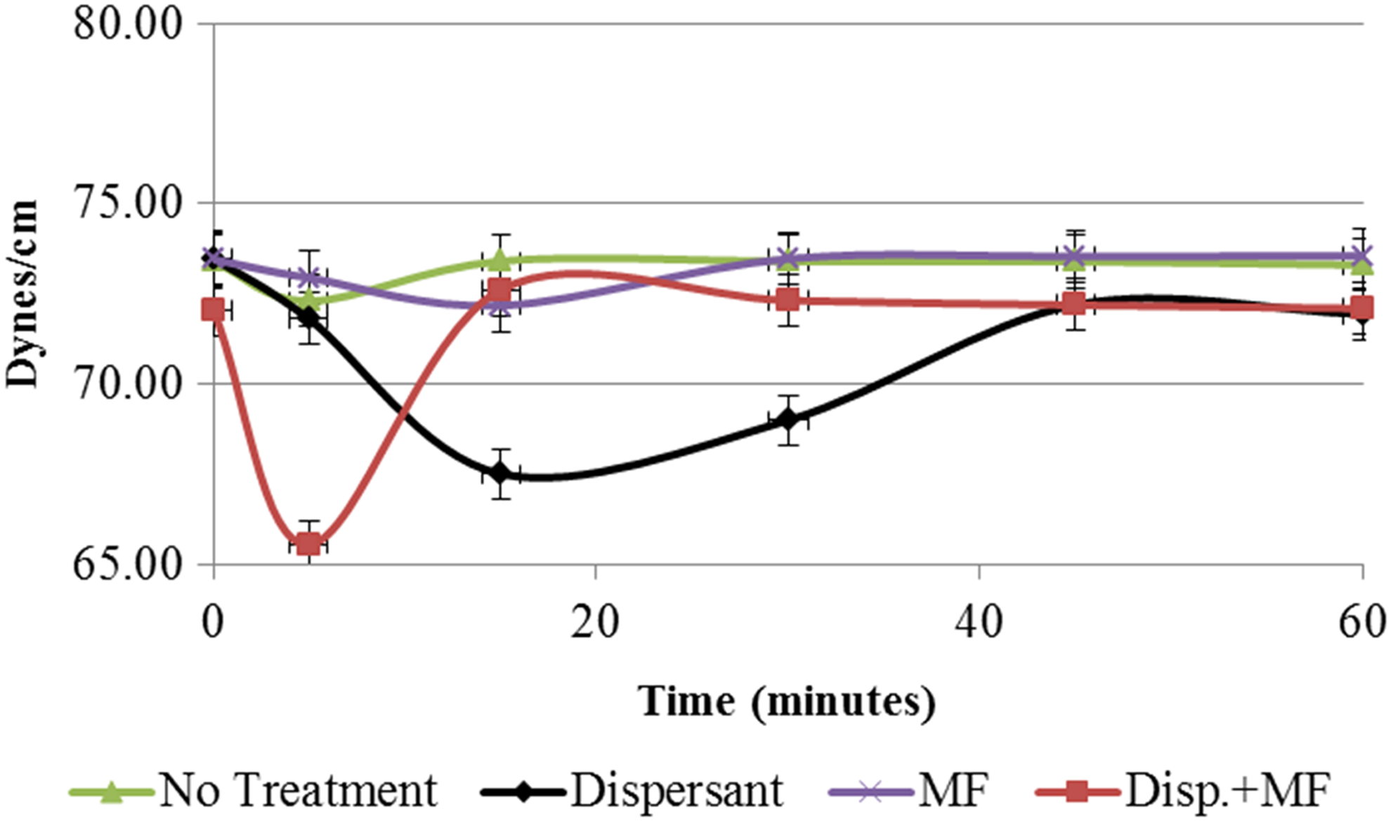
Surface tension measurements of water-air were performed on all collected seawater samples to assess the dispersion of nonconventional oils in the subsurface water column. This technique to evaluate oil dispersion has been previously used by King et al. (2013). In breaking wave conditions, the mean surface tension measurements from three depths at a sampling location 1,200 cm downstream of oil release were plotted against time (Figs. 8 and 9) for each of the four treatments applied to the CLB.

OPEN IN VIEWER

FIG. 8.

Springtime experiments: interfacial tension measurements (average of all depths at location D) of seawater samples collected at various time points during the experiment with CLB.

OPEN IN VIEWER

FIG. 9.

Summertime experiments: interfacial tension measurements (average of all depths at location D) of seawater samples collected at various time points during the experiment with CLB.

In both spring and summer experiments (Figs. 8 and 9), no treatment and MF only provided insufficient dispersion of CLB; therefore, these treatments had a minimal effect on the surface tension of the seawater. However, chemical dispersant enhanced the dispersions of CLB, resulting in a decrease in the interfacial tension of dispersed CLB in seawater. It is important to note that dispersants are surfactants, which are formulated to lower surface tension at the air/water boundary. For the dispersant+MF experiments, only a slight decrease in the interfacial tension was noted in the spring (Fig. 8), but a decrease of more than 10% was observed at 5 min in the summer experiments (Fig. 9). We could not explain the lack of decrease in the spring experiments. However, it could be interpreted that summer water temperatures enhanced the dispersion/dissolution of TPHs, thus causing a greater decease in interfacial tension during the summer experiments. The change in the interfacial tension of dispersed CLB in seawater was more gradual when dispersant only was used. This suggests that the dispersant only treatment is more effective in the dispersion of CLB.

Dispersion effectiveness

Calculations pertaining to dispersion effectiveness (DE) can be obtained from Li et al. (2010) and the Government of Canada (2013). The averaged hydrocarbon values for all depths at each sampling location (A, B, C, and D) were used to generate DE (%) values. Briefly, DE [Eq. (1)] over the duration of the entire experiment can be evaluated by computing the fraction of dispersed oil purged from the wave tank [P(%); Eq. (2)] and the residual dispersed oil in the water column [D_wc (%); Eq. (3)] at the end of each experiment: \documentclass{aastex}\usepackage{amsbsy}\usepackage{amsfonts}\usepackage{amssymb}\usepackage{bm}\usepackage{mathrsfs}\usepackage{pifont}\usepackage{stmaryrd}\usepackage{textcomp}\usepackage{portland, xspace}\usepackage{amsmath, amsxtra}\pagestyle{empty}\DeclareMathSizes{10}{9}{7}{6}\begin{document} \begin{align*}DE ( \% ) = P ( \% ) + D_{wc} ( \% ) \tag{1}\end{align*} \end{document} \documentclass{aastex}\usepackage{amsbsy}\usepackage{amsfonts}\usepackage{amssymb}\usepackage{bm}\usepackage{mathrsfs}\usepackage{pifont}\usepackage{stmaryrd}\usepackage{textcomp}\usepackage{portland, xspace}\usepackage{amsmath, amsxtra}\pagestyle{empty}\DeclareMathSizes{10}{9}{7}{6}\begin{document} \begin{align*}P ( \% ) = \frac { \overline { C } _ { effluent } Q_ { effluent } T } { M_ { Oil } } \times 100 ( \% ) \tag { 2 } \end{align*} \end{document} \documentclass{aastex}\usepackage{amsbsy}\usepackage{amsfonts}\usepackage{amssymb}\usepackage{bm}\usepackage{mathrsfs}\usepackage{pifont}\usepackage{stmaryrd}\usepackage{textcomp}\usepackage{portland, xspace}\usepackage{amsmath, amsxtra}\pagestyle{empty}\DeclareMathSizes{10}{9}{7}{6}\begin{document} \begin{align*}D_ { wc } ( \% ) = \frac { \overline { C } _ { sample } V_ { wt } } { M_ { Oil } } \times 100 ( \% ) \tag { 3 } \end{align*} \end{document}

where \documentclass{aastex}\usepackage{amsbsy}\usepackage{amsfonts}\usepackage{amssymb}\usepackage{bm}\usepackage{mathrsfs}\usepackage{pifont}\usepackage{stmaryrd}\usepackage{textcomp}\usepackage{portland, xspace}\usepackage{amsmath, amsxtra}\pagestyle{empty}\DeclareMathSizes{10}{9}{7}{6}\begin{document} $$\overline{C}_{effluent}$$ \end{document} is the time-averaged oil concentration in the effluent carried out of the wave tank (g/L); \documentclass{aastex}\usepackage{amsbsy}\usepackage{amsfonts}\usepackage{amssymb}\usepackage{bm}\usepackage{mathrsfs}\usepackage{pifont}\usepackage{stmaryrd}\usepackage{textcomp}\usepackage{portland, xspace}\usepackage{amsmath, amsxtra}\pagestyle{empty}\DeclareMathSizes{10}{9}{7}{6}\begin{document} $$Q_{effluent}$$ \end{document} is the flow rate of the current (L/min); V_wt is total effective water volume of the wave tank (28,800 L); T is the duration of each wave tank experiment (60 min); \documentclass{aastex}\usepackage{amsbsy}\usepackage{amsfonts}\usepackage{amssymb}\usepackage{bm}\usepackage{mathrsfs}\usepackage{pifont}\usepackage{stmaryrd}\usepackage{textcomp}\usepackage{portland, xspace}\usepackage{amsmath, amsxtra}\pagestyle{empty}\DeclareMathSizes{10}{9}{7}{6}\begin{document} $$\overline{C}_{sample}$$ \end{document} represents the average concentration of oil remaining in the water column after T; and M_oil is the mass of oil used in the experiment.

Figure 10 demonstrates the dispersion of the CLB dilbit product under the influence of oil spill treating agents under breaking waves and seasonal environmental conditions. Of the oil spill treating agents studied, chemical dispersant application to the CLB was proven to be most effective for dispersing the product in seawater under our test conditions. These data were supported by the LISST particle size distribution data where the majority of the particles produced were <70 μm when dispersant alone was applied to CLB. Under summertime environmental conditions, dispersant application removed more of the oil from the water surface compared with springtime conditions.

OPEN IN VIEWER

FIG. 10.

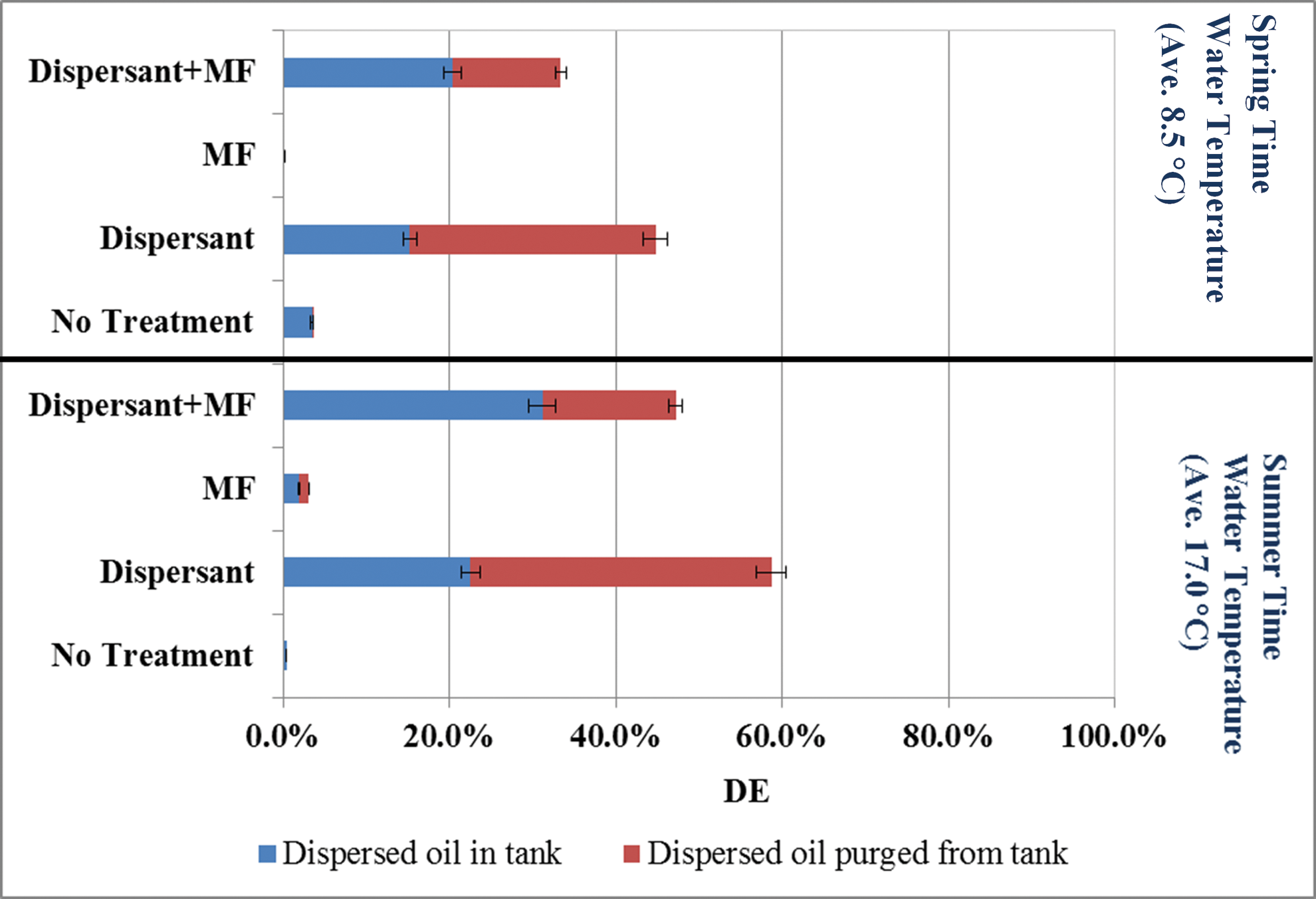
Effectiveness of oil spill treating agents applied to the CLB dilbit product under seasonal conditions in the presence of breaking waves and currents.

Table 2 reports the results of the randomization test. For the spring experiments, the dispersant alone seems to cause most of the dispersion of CLB at a high significance level (p<0.01). For the summer experiments, dispersant alone had the greatest effects (difference of more than 50% with the base case) on the dispersion of CLB at a very high significance level (p<0.009). This was followed by dispersant+MF where the difference was more than 40% at a high significance level (p<0.005). Thus, this suggests that the addition of dispersant+MF is most effective under high temperature (i.e., in the summer).