Sedimentation Behavior of Dispersions Composed of Large and Small Charged Colloidal Particles: Development of New Technology to Improve the Visibility of Small Lakes and Ponds

Particle model

A variety of clay materials and other materials such as corrupt plants may be considered as dirty particles that worsen the visibility of lakes and ponds. Actual dirty particles are supposed to be mixtures of these materials, which are strongly dependent on individual local circumstances of lakes and ponds. Hence, exact material quantities including the shape will be determined when we concretely tackle visibility problems of water in a local lake or pond.

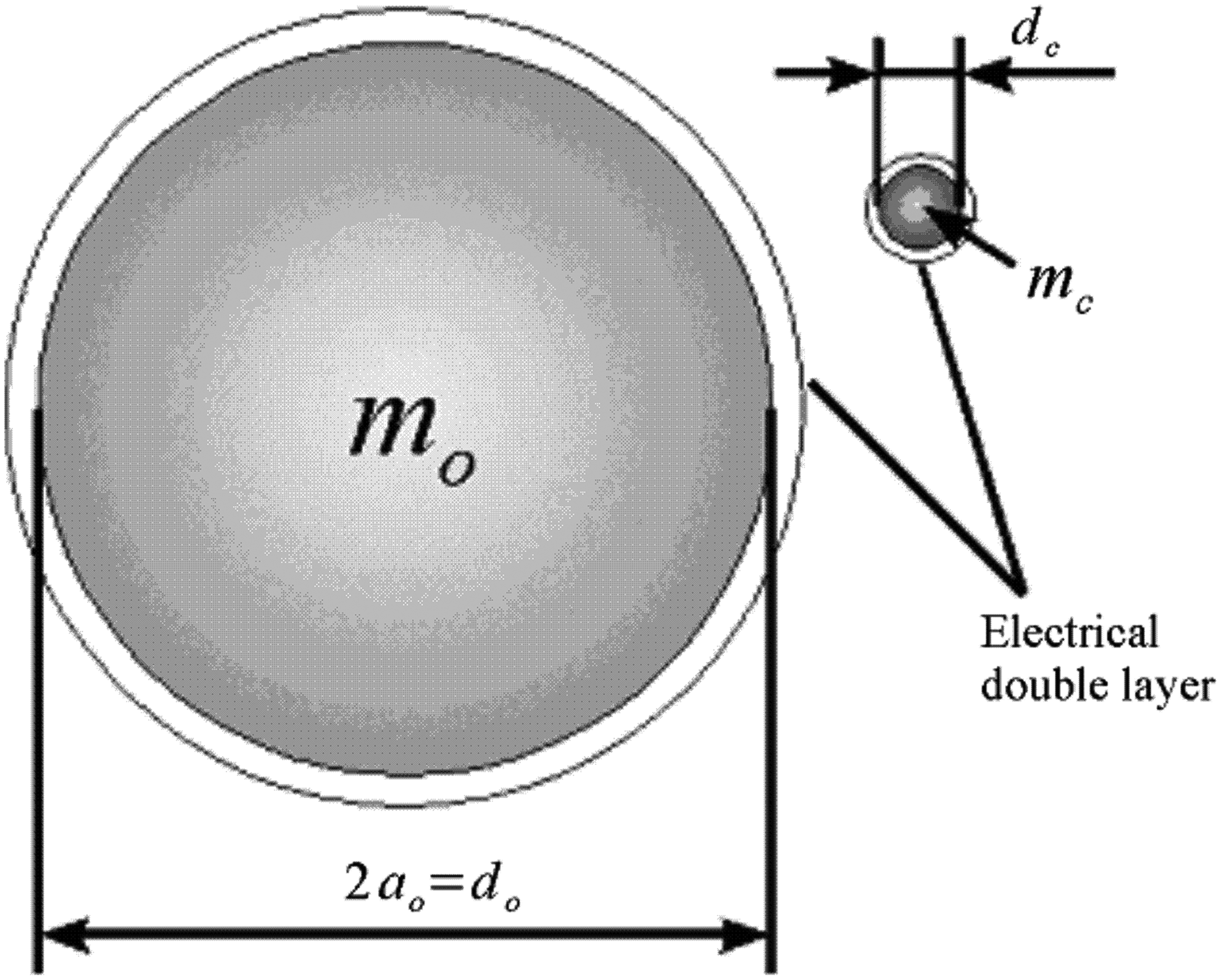
In this study, dirty particles (called small particles below) are modeled as a charged small spherical particle and adsorbing particles (called large particles below) are done as an oppositely charged large spherical particle, as shown in Fig. 1. These particles are assumed to be both of approximately micron-order or smaller, and therefore the Brownian motion of the particles have to be taken into account in simulations. Here, subscripts c and o are used for denoting quantities of charged small spherical particles and oppositely charged large spherical particles, respectively. Dirty particles with diameter d_c have a mass m_c and adsorbing particles with diameter d_o have a mass m_o. The Derjaguin-Landau-Verwey-Overbeek (DVLO) theory and the hetero aggregation theory (Kitahara and Watanabe, 1972; Tachibana et al., 1981; Kitahara, 1994) are used for electrical particle–particle interactions, denoted by V^R. Moreover, the van der Waals interaction energy is taken into account, denoted by V^A; this interaction is not due to electrical properties of particles. The net interaction energy V^net between two charged particles will be the sum of the electrical and the van der Waals interaction energies, that is, V^net=V^R+V^A. The expressions of these energies will be shown below.

OPEN IN VIEWER

FIG. 1.

Particle model.

Interaction energy due to overlap of electrical double layers

DLVO theory and the hetero aggregation theory (Kitahara and Watanabe, 1972; Tachibana et al., 1981; Kitahara, 1994) are based on the diffuse double layer model that was presented by Gouy-Chapman. In this diffuse double layer model, ions are assumed to be a point charge and the density of ions around each dispersed particle is assumed to be followed by the Boltzmann distribution, in which the solvent is treated as a continuum medium with fixed dielectric constant. This model enables one to express an electric potential distribution near a plate as a solution of the Poisson-Boltzmann equation. Since the basic equation, however, is nonlinear, the solution is obtained by introducing Debye-Hückel approximation, which yields the linearized equation. In addition, the Derjaguin approximation gives rise to an interaction energy for the two spherical particles. We now show these expressions in the following paragraph.

For the same kind of spherical particles, for example, for two small particles, an expression for the interaction due to the overlap of the electrical double layers, \documentclass{aastex}\usepackage{amsbsy}\usepackage{amsfonts}\usepackage{amssymb}\usepackage{bm}\usepackage{mathrsfs}\usepackage{pifont}\usepackage{stmaryrd}\usepackage{textcomp}\usepackage{portland, xspace}\usepackage{amsmath, amsxtra}\pagestyle{empty}\DeclareMathSizes{10}{9}{7}{6}\begin{document} $$V_{c - c}^R$$ \end{document} , is expressed as (Kitahara and Watanabe, 1972; Tachibana et al., 1981; Kitahara, 1994) \documentclass{aastex}\usepackage{amsbsy}\usepackage{amsfonts}\usepackage{amssymb}\usepackage{bm}\usepackage{mathrsfs}\usepackage{pifont}\usepackage{stmaryrd}\usepackage{textcomp}\usepackage{portland, xspace}\usepackage{amsmath, amsxtra}\pagestyle{empty}\DeclareMathSizes{10}{9}{7}{6}\begin{document} \begin{align*}V_{c - c}^R = 2 \pi \varepsilon a_c \psi_c^2 \; { \rm ln} \left[ 1 + { \rm exp} \{ - \kappa ( r - 2 a_c ) \} \right] \tag{1}\end{align*} \end{document}

in which \documentclass{aastex}\usepackage{amsbsy}\usepackage{amsfonts}\usepackage{amssymb}\usepackage{bm}\usepackage{mathrsfs}\usepackage{pifont}\usepackage{stmaryrd}\usepackage{textcomp}\usepackage{portland, xspace}\usepackage{amsmath, amsxtra}\pagestyle{empty}\DeclareMathSizes{10}{9}{7}{6}\begin{document} \begin{align*}\kappa = \sqrt { \frac { 2000e^2 z^2 N_A C } { \varepsilon k_B T } } \tag { 2 } \end{align*} \end{document}

An expression for the two large particles is obtained by replacing subscript c with o in Equation (1). In Equations (1) and (2), r is the center-to-center separation between the two particles, ɛ is the dielectric constant of the solvent, a_c is the radius of the small spherical particles, ψ_c is the surface potential of the small spherical particles, and κ is the Debye parameter (the reciprocal number 1/κ corresponds to the thickness of the electrical double layer). Also, e is the elementary electric charge, z is the ionic valency, N_A is the Avogadro number, C is the concentration of the electrolyte, k_B is Boltzmann's constant, and T is the temperature of the suspension.

For different kinds of particles, an interaction energy \documentclass{aastex}\usepackage{amsbsy}\usepackage{amsfonts}\usepackage{amssymb}\usepackage{bm}\usepackage{mathrsfs}\usepackage{pifont}\usepackage{stmaryrd}\usepackage{textcomp}\usepackage{portland, xspace}\usepackage{amsmath, amsxtra}\pagestyle{empty}\DeclareMathSizes{10}{9}{7}{6}\begin{document} $$V_{c - o}^R$$ \end{document} due to the overlap of the electrical double layers was given by Hogg et al. (1966) as \documentclass{aastex}\usepackage{amsbsy}\usepackage{amsfonts}\usepackage{amssymb}\usepackage{bm}\usepackage{mathrsfs}\usepackage{pifont}\usepackage{stmaryrd}\usepackage{textcomp}\usepackage{portland, xspace}\usepackage{amsmath, amsxtra}\pagestyle{empty}\DeclareMathSizes{10}{9}{7}{6}\begin{document} \begin{align*}\begin{split}V_{c - o}^R = & \frac {\pi \varepsilon\; a_c\; a_o\; ( \psi_c^2 + \psi_o^2 )} {a_c + a_o} \\ & \times \ \bigg \{ \frac {2 \psi_c \psi_o} {\psi_c^2 + \psi_o^2} { \rm ln} \left( \frac {1 + { \rm exp} \{ - \kappa ( r - ( a_c + a_o ) ) \}} {1 - { \rm exp} \{ - \kappa ( r - ( a_c + a_o ) ) \} } \right) \\ & + { \rm ln} [ 1 - { \rm exp} \{ - 2 \kappa ( r - ( a_c + a_o ) ) \} ] \bigg \} \end{split} \tag { 3 } \end{align*} \end{document}

van der Waals interaction energy

The van der Waals force is of short range order in such a way that the potential energy is inversely proportional to the 6th power of the inter-atomic distance. However, the summation of all interactions between constituent atoms of the two particles leads to a relatively long-range order interaction between the two dispersed particles. Hamaker showed an expression of the interaction energy \documentclass{aastex}\usepackage{amsbsy}\usepackage{amsfonts}\usepackage{amssymb}\usepackage{bm}\usepackage{mathrsfs}\usepackage{pifont}\usepackage{stmaryrd}\usepackage{textcomp}\usepackage{portland, xspace}\usepackage{amsmath, amsxtra}\pagestyle{empty}\DeclareMathSizes{10}{9}{7}{6}\begin{document} $$V_{c - c}^A$$ \end{document} between the same kinds of two particles as (Kitahara and Watanabe, 1972; Tachibana et al., 1981; Kitahara, 1994) \documentclass{aastex}\usepackage{amsbsy}\usepackage{amsfonts}\usepackage{amssymb}\usepackage{bm}\usepackage{mathrsfs}\usepackage{pifont}\usepackage{stmaryrd}\usepackage{textcomp}\usepackage{portland, xspace}\usepackage{amsmath, amsxtra}\pagestyle{empty}\DeclareMathSizes{10}{9}{7}{6}\begin{document} \begin{align*}V_ { c - c } ^A = - \frac { A } { 6 } \left[ \frac { 2a_c^2 } { r^2 - 4a_c^2 } + \frac { 2a_c^2 } { r^2 } + { \rm ln } \left( \frac { r^2 - 4a_c^2 } { r^2 } \right) \right] \tag { 4 } \end{align*} \end{document}

and for the case of the different kinds of particles, the interaction energy \documentclass{aastex}\usepackage{amsbsy}\usepackage{amsfonts}\usepackage{amssymb}\usepackage{bm}\usepackage{mathrsfs}\usepackage{pifont}\usepackage{stmaryrd}\usepackage{textcomp}\usepackage{portland, xspace}\usepackage{amsmath, amsxtra}\pagestyle{empty}\DeclareMathSizes{10}{9}{7}{6}\begin{document} $$V_{c - o}^A$$ \end{document} is expressed as \documentclass{aastex}\usepackage{amsbsy}\usepackage{amsfonts}\usepackage{amssymb}\usepackage{bm}\usepackage{mathrsfs}\usepackage{pifont}\usepackage{stmaryrd}\usepackage{textcomp}\usepackage{portland, xspace}\usepackage{amsmath, amsxtra}\pagestyle{empty}\DeclareMathSizes{10}{9}{7}{6}\begin{document} \begin{align*}\begin{split}V_{c - o}^A = & - \frac {A} {6} \bigg[ \frac {2a_c a_o} {r^{2}-( a_c + a_o )^2} + \frac {2a_c a_o} {r^{2} - ( a_c - a_o )^2} \\& + {\rm ln} \left( \frac {r^{2} - (a_c + a_o )^2} {r^{2} - (a_c - a_o)^2} \right) \bigg]\end{split} \tag{5}\end{align*} \end{document}

in which A is the Hamaker constant. In the present suspension, the effective Hamaker constant has to be evaluated by taking into account the effect of the solvent molecules. We now use the notation A_c-c for the Hamaker constant of the interaction between the two small particles, A_o-o for the interaction between the two large particles, and A^(w) for the characteristic of water; it is noted that A_c-c and A_o-o are for the case of no water. Employing this notation, under the circumstance of solvent medium (water), the Hamaker constants \documentclass{aastex}\usepackage{amsbsy}\usepackage{amsfonts}\usepackage{amssymb}\usepackage{bm}\usepackage{mathrsfs}\usepackage{pifont}\usepackage{stmaryrd}\usepackage{textcomp}\usepackage{portland, xspace}\usepackage{amsmath, amsxtra}\pagestyle{empty}\DeclareMathSizes{10}{9}{7}{6}\begin{document} $$A_{c - c}^{ ( w ) }$$ \end{document} , \documentclass{aastex}\usepackage{amsbsy}\usepackage{amsfonts}\usepackage{amssymb}\usepackage{bm}\usepackage{mathrsfs}\usepackage{pifont}\usepackage{stmaryrd}\usepackage{textcomp}\usepackage{portland, xspace}\usepackage{amsmath, amsxtra}\pagestyle{empty}\DeclareMathSizes{10}{9}{7}{6}\begin{document} $$A_{o - o}^{ ( w ) }$$ \end{document} , and \documentclass{aastex}\usepackage{amsbsy}\usepackage{amsfonts}\usepackage{amssymb}\usepackage{bm}\usepackage{mathrsfs}\usepackage{pifont}\usepackage{stmaryrd}\usepackage{textcomp}\usepackage{portland, xspace}\usepackage{amsmath, amsxtra}\pagestyle{empty}\DeclareMathSizes{10}{9}{7}{6}\begin{document} $$A_{c - o}^{ ( w ) }$$ \end{document} for the interaction between small particles, between large particles, and between small and large particles, respectively, are expressed as \documentclass{aastex}\usepackage{amsbsy}\usepackage{amsfonts}\usepackage{amssymb}\usepackage{bm}\usepackage{mathrsfs}\usepackage{pifont}\usepackage{stmaryrd}\usepackage{textcomp}\usepackage{portland, xspace}\usepackage{amsmath, amsxtra}\pagestyle{empty}\DeclareMathSizes{10}{9}{7}{6}\begin{document} \begin{align*} \begin{split}A_{c - c}^{ ( w ) } = & \left( \sqrt{A_{c - c}} - \sqrt{A^{ ( w ) }} \right) ^2 , \\ A_{o - o}^{ ( w ) } = & \left( \sqrt{A_{o - o}} - \sqrt{A^{ ( w ) }} \right) ^2 , \\ A_{c - o}^{ ( w ) } = & \left( \sqrt{A_{c - c}} - \sqrt{A^{ ( w ) }} \right) \left( \sqrt{A_{o - o}} - \sqrt{A^{ ( w ) }} \right).\end{split} \tag{6}\end{align*} \end{document}

It is noted that the values of the Hamaker constant of various materials are already listed in the typical textbook of colloidal dispersion, and are usually of the order of 10⁻²⁰ ∼10⁻¹⁹ J.

Kinetic equation of particles

Both the small and the large particles perform Brownian motion in a real situation, and therefore the Brownian dynamics method (Satoh, 2003, 2010) is here employed to simulate these particles under the situation of the gravity field. As already mentioned in the Introduction, we focus on the improvement of the visibility of small lakes or ponds, so that we treat the sedimentation phenomenon in a quiescent flow situation of the ambient liquid. Moreover, it is assumed that the temperature is constant in the whole system because we address the sedimentation phenomenon in a significantly simplified system that is modeled for representing a small and shallow lake or pond.

In the present spherical particle system, the translation motion is a governing factor of the sedimentation phenomenon of particles, so that we do not taken into consideration the rotational motion of particles; the main objective of this study is to investigate the influence of the activity of translational Brownian motion of the large particles on the performance of the adsorption rate. If nonspherical particles such as rod-like or plate-like particles are used as large particles, rotational Brownian motion is expected to become an important factor in addition to the translational Brownian motion.

Since it is quite difficult to treat multi-body hydrodynamic interactions among particles even for a spherical particle suspension, we here neglect these hydrodynamic interactions; this simplified approach is frequently employed as the first approximation for investigating the physical phenomenon of interest in the field of simulation-based researches, in particular for the case of nonspherical particle suspensions. If the velocity vector of an arbitrary small particle i is denoted by v _ci , the nonhydrodynamic force by \documentclass{aastex}\usepackage{amsbsy}\usepackage{amsfonts}\usepackage{amssymb}\usepackage{bm}\usepackage{mathrsfs}\usepackage{pifont}\usepackage{stmaryrd}\usepackage{textcomp}\usepackage{portland, xspace}\usepackage{amsmath, amsxtra}\pagestyle{empty}\DeclareMathSizes{10}{9}{7}{6}\begin{document} $$\textbf{\textit{{F}}}_{ci}^p$$ \end{document} and the random force by \documentclass{aastex}\usepackage{amsbsy}\usepackage{amsfonts}\usepackage{amssymb}\usepackage{bm}\usepackage{mathrsfs}\usepackage{pifont}\usepackage{stmaryrd}\usepackage{textcomp}\usepackage{portland, xspace}\usepackage{amsmath, amsxtra}\pagestyle{empty}\DeclareMathSizes{10}{9}{7}{6}\begin{document} $$\textbf{\textit{{F}}}_{ci}^B$$ \end{document} , then the equation of motion of particle i (similarly, of large particle j) is expressed as (Satoh, 2003, 2010) \documentclass{aastex}\usepackage{amsbsy}\usepackage{amsfonts}\usepackage{amssymb}\usepackage{bm}\usepackage{mathrsfs}\usepackage{pifont}\usepackage{stmaryrd}\usepackage{textcomp}\usepackage{portland, xspace}\usepackage{amsmath, amsxtra}\pagestyle{empty}\DeclareMathSizes{10}{9}{7}{6}\begin{document} \begin{align*} { m } _c \frac { d \boldsymbol{\nu } _ { ci } } { dt } = - \xi_c \boldsymbol {\nu} _ { ci } + \textbf{\textit{F}} _ { ci } ^P + \textbf{\textit{F}} _ { ci } ^B \tag { 7 } \end{align*} \end{document} \documentclass{aastex}\usepackage{amsbsy}\usepackage{amsfonts}\usepackage{amssymb}\usepackage{bm}\usepackage{mathrsfs}\usepackage{pifont}\usepackage{stmaryrd}\usepackage{textcomp}\usepackage{portland, xspace}\usepackage{amsmath, amsxtra}\pagestyle{empty}\DeclareMathSizes{10}{9}{7}{6}\begin{document} \begin{align*} { m } _o \frac { d \boldsymbol{\nu} _ { oj } } { dt } = - \xi_o \boldsymbol{\nu} _ { oj } + \textbf{\textit{F}} _ { oj } ^P + \textbf{\textit{F}} _ { oj } ^B \tag {8}\end{align*} \end{document}

in which m_c is the mass of the particles, and ξ_c is the friction coefficient, expressed as ξ_c=3πηd_c (η is the liquid viscosity); it is noted that subscripts i and k are used for small particles, and j and l are for large particles in the following expressions. Moreover, \documentclass{aastex}\usepackage{amsbsy}\usepackage{amsfonts}\usepackage{amssymb}\usepackage{bm}\usepackage{mathrsfs}\usepackage{pifont}\usepackage{stmaryrd}\usepackage{textcomp}\usepackage{portland, xspace}\usepackage{amsmath, amsxtra}\pagestyle{empty}\DeclareMathSizes{10}{9}{7}{6}\begin{document} $$\textbf{\textit{F}}_{ci}^p$$ \end{document} is the sum of the force exerted by the ambient particles and the force by the external forces of gravity and buoyancy, and \documentclass{aastex}\usepackage{amsbsy}\usepackage{amsfonts}\usepackage{amssymb}\usepackage{bm}\usepackage{mathrsfs}\usepackage{pifont}\usepackage{stmaryrd}\usepackage{textcomp}\usepackage{portland, xspace}\usepackage{amsmath, amsxtra}\pagestyle{empty}\DeclareMathSizes{10}{9}{7}{6}\begin{document} $$\textbf{\textit{F}}_{ci}^B$$ \end{document} is the random force inducing the particle Brownian motion. The inertial term is generally negligible for a colloidal dispersion, and therefore Equations (7) and (8) reduce to the following equations: \documentclass{aastex}\usepackage{amsbsy}\usepackage{amsfonts}\usepackage{amssymb}\usepackage{bm}\usepackage{mathrsfs}\usepackage{pifont}\usepackage{stmaryrd}\usepackage{textcomp}\usepackage{portland, xspace}\usepackage{amsmath, amsxtra}\pagestyle{empty}\DeclareMathSizes{10}{9}{7}{6}\begin{document} \begin{align*} \boldsymbol{\nu} _ { ci } = \frac { 1 } { \xi_c } ( \textbf{\textit{F} } _ { ci } ^P + \textbf{\textit{F}} _ { ci } ^B ) \tag { 9 } \end{align*} \end{document} \documentclass{aastex}\usepackage{amsbsy}\usepackage{amsfonts}\usepackage{amssymb}\usepackage{bm}\usepackage{mathrsfs}\usepackage{pifont}\usepackage{stmaryrd}\usepackage{textcomp}\usepackage{portland, xspace}\usepackage{amsmath, amsxtra}\pagestyle{empty}\DeclareMathSizes{10}{9}{7}{6}\begin{document} \begin{align*} \boldsymbol{\nu} _ { oj } = \frac { 1 } { \xi_o } ( \textbf{\textit {F}} _ { oj } ^P + \textbf{\textit{F}} _ { oj } ^B ) \tag { 10 } \end{align*} \end{document}

The finite difference equation governing the particle position after a time interval Δt is obtained from Equations (9) and (10) as \documentclass{aastex}\usepackage{amsbsy}\usepackage{amsfonts}\usepackage{amssymb}\usepackage{bm}\usepackage{mathrsfs}\usepackage{pifont}\usepackage{stmaryrd}\usepackage{textcomp}\usepackage{portland, xspace}\usepackage{amsmath, amsxtra}\pagestyle{empty}\DeclareMathSizes{10}{9}{7}{6}\begin{document} \begin{align*}\textbf{\textit{r}} _ { ci } ( t + \Delta t ) = \textbf{\textit{r}} _ {ci} ( t ) + \frac { 1 } { \xi_c } \Delta t \textbf{\textit{F}} _ { ci } ^P + \Delta r_ { ci } ^B \tag { 11 } \end{align*} \end{document} \documentclass{aastex}\usepackage{amsbsy}\usepackage{amsfonts}\usepackage{amssymb}\usepackage{bm}\usepackage{mathrsfs}\usepackage{pifont}\usepackage{stmaryrd}\usepackage{textcomp}\usepackage{portland, xspace}\usepackage{amsmath, amsxtra}\pagestyle{empty}\DeclareMathSizes{10}{9}{7}{6}\begin{document} \begin{align*}\textbf{\textit{r}} _ { oj } ( t + \Delta t ) = \textbf{\textit{r}} _ { oj } ( t ) + \frac { 1 } { \xi_o } \Delta t \textbf{\textit{F }}^{P}_ {oj} + \Delta \textbf{\textit{r}} _ { oj } ^B \tag { 12 } \end{align*} \end{document}

in which \documentclass{aastex}\usepackage{amsbsy}\usepackage{amsfonts}\usepackage{amssymb}\usepackage{bm}\usepackage{mathrsfs}\usepackage{pifont}\usepackage{stmaryrd}\usepackage{textcomp}\usepackage{portland, xspace}\usepackage{amsmath, amsxtra}\pagestyle{empty}\DeclareMathSizes{10}{9}{7}{6}\begin{document} $$\Delta \textbf{\textit{r}}_{ci}^B$$ \end{document} and \documentclass{aastex}\usepackage{amsbsy}\usepackage{amsfonts}\usepackage{amssymb}\usepackage{bm}\usepackage{mathrsfs}\usepackage{pifont}\usepackage{stmaryrd}\usepackage{textcomp}\usepackage{portland, xspace}\usepackage{amsmath, amsxtra}\pagestyle{empty}\DeclareMathSizes{10}{9}{7}{6}\begin{document} $$\Delta \textbf{\textit{r}}_{oj}^B$$ \end{document} are the random displacements inducing the Brownian motion of small and large particles, respectively. These quantities are related to the system temperature and the viscosity in a stochastic manner, as shown in Equations (23) and (24); it is noted that the random displacement is larger with increasing system temperature and decreasing particle diameter. These expressions in Equations (11) and (12) are the basic equations for simulating the translational Brownian motion of the particles in the situation where multi-body hydrodynamic interactions among particles are neglected and a macroscopic flow of the ambient liquid can be regarded as negligible.

The nonrandom forces acting on small particle i and large particle j are expressed, respectively, as \documentclass{aastex}\usepackage{amsbsy}\usepackage{amsfonts}\usepackage{amssymb}\usepackage{bm}\usepackage{mathrsfs}\usepackage{pifont}\usepackage{stmaryrd}\usepackage{textcomp}\usepackage{portland, xspace}\usepackage{amsmath, amsxtra}\pagestyle{empty}\DeclareMathSizes{10}{9}{7}{6}\begin{document} \begin{align*}\textbf{\textit{F}}_{ci}^P = \textbf{\textit{F}}_{ci}^G + \sum_k \Big ( \textbf{\textit{F}}_{ci - ck}^R + \textbf{\textit{F}}_{ci - ck}^A \Big ) + \sum_l \Big ( \textbf{\textit{F}}_{ci - ol}^R + \textbf{\textit{F}}_{ci - ol}^A \Big ) \tag{13}\end{align*} \end{document} \documentclass{aastex}\usepackage{amsbsy}\usepackage{amsfonts}\usepackage{amssymb}\usepackage{bm}\usepackage{mathrsfs}\usepackage{pifont}\usepackage{stmaryrd}\usepackage{textcomp}\usepackage{portland, xspace}\usepackage{amsmath, amsxtra}\pagestyle{empty}\DeclareMathSizes{10}{9}{7}{6}\begin{document} \begin{align*}\textbf{\textit{F}}_{oj}^P = \textbf{\textit{F}}_{oj}^G + \sum_k \Big ( \textbf{\textit{F}}_{oj - ck}^R + \textbf{\textit{F}}_{oj - ck}^A \Big) + \sum_l \Big ( \textbf{\textit{F}}_{oj - ol}^R + \textbf{\textit{F}}_{oj - ol}^A \Big ) \tag{14}\end{align*} \end{document}

The force \documentclass{aastex}\usepackage{amsbsy}\usepackage{amsfonts}\usepackage{amssymb}\usepackage{bm}\usepackage{mathrsfs}\usepackage{pifont}\usepackage{stmaryrd}\usepackage{textcomp}\usepackage{portland, xspace}\usepackage{amsmath, amsxtra}\pagestyle{empty}\DeclareMathSizes{10}{9}{7}{6}\begin{document} $$\textbf{\textit{F}}_{ci}^G$$ \end{document} and \documentclass{aastex}\usepackage{amsbsy}\usepackage{amsfonts}\usepackage{amssymb}\usepackage{bm}\usepackage{mathrsfs}\usepackage{pifont}\usepackage{stmaryrd}\usepackage{textcomp}\usepackage{portland, xspace}\usepackage{amsmath, amsxtra}\pagestyle{empty}\DeclareMathSizes{10}{9}{7}{6}\begin{document} $$\textbf{\textit{F}}_{oj}^G$$ \end{document} due to both gravity field and buoyancy are expressed as \documentclass{aastex}\usepackage{amsbsy}\usepackage{amsfonts}\usepackage{amssymb}\usepackage{bm}\usepackage{mathrsfs}\usepackage{pifont}\usepackage{stmaryrd}\usepackage{textcomp}\usepackage{portland, xspace}\usepackage{amsmath, amsxtra}\pagestyle{empty}\DeclareMathSizes{10}{9}{7}{6}\begin{document} \begin{align*}\textbf{\textit{F}}_{ci}^G = { m}_c \textbf{\textit{g}} - \rho_f V_c \textbf{\textit{g}} \tag{15}\end{align*} \end{document} \documentclass{aastex}\usepackage{amsbsy}\usepackage{amsfonts}\usepackage{amssymb}\usepackage{bm}\usepackage{mathrsfs}\usepackage{pifont}\usepackage{stmaryrd}\usepackage{textcomp}\usepackage{portland, xspace}\usepackage{amsmath, amsxtra}\pagestyle{empty}\DeclareMathSizes{10}{9}{7}{6}\begin{document} \begin{align*}\textbf{\textit{F}}_{oj}^G = { m}_o \textbf{\textit{g}} - \rho_f V_o \textbf{\textit{g}} \tag{16}\end{align*} \end{document}

in which g (g=| g |) is the gravitational acceleration, V_c is the volume of a small particle, and ρ_f is the density of the fluid. The force due to the electrical interaction between the small particles i and k, \documentclass{aastex}\usepackage{amsbsy}\usepackage{amsfonts}\usepackage{amssymb}\usepackage{bm}\usepackage{mathrsfs}\usepackage{pifont}\usepackage{stmaryrd}\usepackage{textcomp}\usepackage{portland, xspace}\usepackage{amsmath, amsxtra}\pagestyle{empty}\DeclareMathSizes{10}{9}{7}{6}\begin{document} $$\textbf{\textit{F}}_{ci - ck}^R$$ \end{document} , and the force due to the van der Waals interaction, \documentclass{aastex}\usepackage{amsbsy}\usepackage{amsfonts}\usepackage{amssymb}\usepackage{bm}\usepackage{mathrsfs}\usepackage{pifont}\usepackage{stmaryrd}\usepackage{textcomp}\usepackage{portland, xspace}\usepackage{amsmath, amsxtra}\pagestyle{empty}\DeclareMathSizes{10}{9}{7}{6}\begin{document} $$\textbf{\textit{F}}_{ci - ck}^A$$ \end{document} , are expressed as \documentclass{aastex}\usepackage{amsbsy}\usepackage{amsfonts}\usepackage{amssymb}\usepackage{bm}\usepackage{mathrsfs}\usepackage{pifont}\usepackage{stmaryrd}\usepackage{textcomp}\usepackage{portland, xspace}\usepackage{amsmath, amsxtra}\pagestyle{empty}\DeclareMathSizes{10}{9}{7}{6}\begin{document} \begin{align*}\textbf{\textit{F}} _ { ci - ck } ^R = 2 \pi \varepsilon \;a_c \psi_c^2 \kappa \;\textbf{\textit{t}} _{r} \frac { { \rm exp } [ - \kappa ( r - 2a_c ) ] } { 1 + { \rm exp } [ - \kappa ( r - 2_ { a_c } ) ] } \tag { 17 } \end{align*} \end{document} \documentclass{aastex}\usepackage{amsbsy}\usepackage{amsfonts}\usepackage{amssymb}\usepackage{bm}\usepackage{mathrsfs}\usepackage{pifont}\usepackage{stmaryrd}\usepackage{textcomp}\usepackage{portland, xspace}\usepackage{amsmath, amsxtra}\pagestyle{empty}\DeclareMathSizes{10}{9}{7}{6}\begin{document} \begin{align*}\textbf{\textit{F}} _ { ci - ck } ^A = \frac { A_ { c - c } ^ { ( w ) } } { 6 } \textbf{\textit{t}}_r \left[ - \frac { 4 a_c^2 r } { ( r^2 - 4 a_c^2 ) ^2 } - \frac { 4 a_c^2 } { r^3 } + \frac { 2 r } { r^2 - 4a_c^2 } - \frac { 2 } { r } \right] \tag { 18 } \end{align*} \end{document}

in which for simplification of expressions, the position vector of particle i relative to particle k (r_ik=| r _ik |) is denoted by r without subscripts (r=| r |); this simplified notation is employed for relative position vectors in the following expressions. It is therefore noted that t _r = r /r in Equation (18) implies t _rik = r _ik / r _ik .

For the case of the large particles, these expressions are written as \documentclass{aastex}\usepackage{amsbsy}\usepackage{amsfonts}\usepackage{amssymb}\usepackage{bm}\usepackage{mathrsfs}\usepackage{pifont}\usepackage{stmaryrd}\usepackage{textcomp}\usepackage{portland, xspace}\usepackage{amsmath, amsxtra}\pagestyle{empty}\DeclareMathSizes{10}{9}{7}{6}\begin{document} \begin{align*}\textbf{\textit{F}} _ { oj - ol } ^R = 2 \pi \varepsilon \;a_o \psi_o^2 \kappa \ \textbf{\textit{t}}_r \frac { \exp [ - \kappa ( r - 2a_o ) ] } { 1 + \exp [ - \kappa ( r - 2a_o ) ] } \tag { 19 } \end{align*} \end{document} \documentclass{aastex}\usepackage{amsbsy}\usepackage{amsfonts}\usepackage{amssymb}\usepackage{bm}\usepackage{mathrsfs}\usepackage{pifont}\usepackage{stmaryrd}\usepackage{textcomp}\usepackage{portland, xspace}\usepackage{amsmath, amsxtra}\pagestyle{empty}\DeclareMathSizes{10}{9}{7}{6}\begin{document} \begin{align*}\textbf{\textit{F}} _ { oj - ol } ^A = \frac { A_ { o - o } ^ { ( w ) } } { 6 } \textbf{\textit{t}} _r \left[ - \frac { 4a_o^2 r } { ( r^2 - 4 a_o^2 ) ^2 } - \frac { 4 a_o^2 } { r^3 } + \frac { 2 r } { r^2 - 4a_o^2 } - \frac { 2 } { r } \right] \tag { 20 } \end{align*} \end{document}

For the case of the inter-particle force between small particle i and large particle l, the forces are expressed as \documentclass{aastex}\usepackage{amsbsy}\usepackage{amsfonts}\usepackage{amssymb}\usepackage{bm}\usepackage{mathrsfs}\usepackage{pifont}\usepackage{stmaryrd}\usepackage{textcomp}\usepackage{portland, xspace}\usepackage{amsmath, amsxtra}\pagestyle{empty}\DeclareMathSizes{10}{9}{7}{6}\begin{document} \begin{align*} \begin{split}\textbf{\textit{F}}_{ci - ol}^R = & \; 2 \kappa \ \textbf{\textit{t}}_r \frac { \pi \varepsilon \; a_c a_o ( \psi_c^2 + \psi_o^2 )} { a_c + a_o} \\ & \times \left\{ \frac { \psi_c \psi_o} {\psi_c^2 + \psi_o^2} \cdot \frac {2 \exp [ - \kappa ( r - ( a_c + a_o ) ) ]} {1 - \exp [ - 2 \kappa ( r - ( a_c + a_o ) ) ] } \right. \\ & \left. - \frac { \exp [ - 2 \kappa ( r - ( a_c + a_o ) ) ]} {1 - \exp [ - 2 \kappa ( r - ( a_c + a_o ) ) ] }\right\} \end{split} \tag{21}\end{align*} \end{document} \documentclass{aastex}\usepackage{amsbsy}\usepackage{amsfonts}\usepackage{amssymb}\usepackage{bm}\usepackage{mathrsfs}\usepackage{pifont}\usepackage{stmaryrd}\usepackage{textcomp}\usepackage{portland, xspace}\usepackage{amsmath, amsxtra}\pagestyle{empty}\DeclareMathSizes{10}{9}{7}{6}\begin{document} \begin{align*}\begin{split}\textbf{\textit{F}}_{ci - ol}^A = & \frac {A_{c - o}^{ ( w ) }} {6} \textbf{\textit{t}}_r \bigg[ - \frac {4a_ca_o r} {\{ r^2 - ( a_c + a_o ) ^2 \} ^2} \\ & - \frac {4a_c a_o r} { \{ r^2 - ( a_c - a_o ) ^2 \} ^2} + \frac {2 r} {r^2 - ( a_c + a_o ) ^2} \quad \\ & - \frac {2r} {r^2 - ( a_c - a_o ) ^2} \bigg]\end{split} \tag{22}\end{align*} \end{document}

Particle displacements due to the Brownian motion, \documentclass{aastex}\usepackage{amsbsy}\usepackage{amsfonts}\usepackage{amssymb}\usepackage{bm}\usepackage{mathrsfs}\usepackage{pifont}\usepackage{stmaryrd}\usepackage{textcomp}\usepackage{portland, xspace}\usepackage{amsmath, amsxtra}\pagestyle{empty}\DeclareMathSizes{10}{9}{7}{6}\begin{document} $$\Delta \textbf{\textit{r}}_{ci}^B$$ \end{document} and \documentclass{aastex}\usepackage{amsbsy}\usepackage{amsfonts}\usepackage{amssymb}\usepackage{bm}\usepackage{mathrsfs}\usepackage{pifont}\usepackage{stmaryrd}\usepackage{textcomp}\usepackage{portland, xspace}\usepackage{amsmath, amsxtra}\pagestyle{empty}\DeclareMathSizes{10}{9}{7}{6}\begin{document} $$\Delta \textbf{\textit{r}}_{oj}^B$$ \end{document} , have the following stochastic properties: \documentclass{aastex}\usepackage{amsbsy}\usepackage{amsfonts}\usepackage{amssymb}\usepackage{bm}\usepackage{mathrsfs}\usepackage{pifont}\usepackage{stmaryrd}\usepackage{textcomp}\usepackage{portland, xspace}\usepackage{amsmath, amsxtra}\pagestyle{empty}\DeclareMathSizes{10}{9}{7}{6}\begin{document} \begin{align*}\big \langle \Delta \textbf{\textit{r}}_{ci}^{B} \big \rangle = 0 , \big \langle \Delta \textbf{\textit{r } } _ { ci } ^B \Delta \textbf{\textit{r}} _ { ci } ^B \big \rangle = 2 \frac { k_B T } { \xi_c } \Delta t \textbf{\textit{I } } \tag { 23 } \end{align*} \end{document} \documentclass{aastex}\usepackage{amsbsy}\usepackage{amsfonts}\usepackage{amssymb}\usepackage{bm}\usepackage{mathrsfs}\usepackage{pifont}\usepackage{stmaryrd}\usepackage{textcomp}\usepackage{portland, xspace}\usepackage{amsmath, amsxtra}\pagestyle{empty}\DeclareMathSizes{10}{9}{7}{6}\begin{document} \begin{align*}\big \langle \Delta \textbf{\textit{r}} _ { oj } ^B \big \rangle = 0 , \big \langle \Delta \textbf{\textit{r} } _ { oj } ^B \Delta \textbf{\textit{r}} _ { oj } ^B \big \rangle = 2 \frac { k_B T } { \xi_o } \Delta t \textbf{\textit{I}} \tag { 24 } \end{align*} \end{document}

in which Δt is the time interval for simulations, I is the unit tensor, and \documentclass{aastex}\usepackage{amsbsy}\usepackage{amsfonts}\usepackage{amssymb}\usepackage{bm}\usepackage{mathrsfs}\usepackage{pifont}\usepackage{stmaryrd}\usepackage{textcomp}\usepackage{portland, xspace}\usepackage{amsmath, amsxtra}\pagestyle{empty}\DeclareMathSizes{10}{9}{7}{6}\begin{document} $$\langle - \rangle$$ \end{document} is the time or ensemble average.

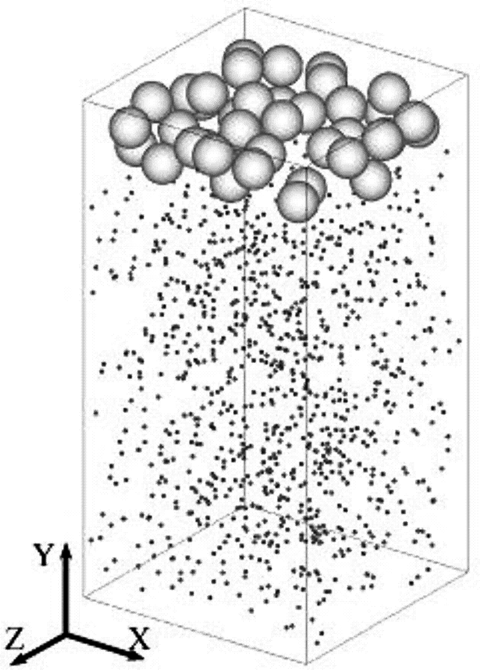
We now briefly describe the boundary conditions that were employed in the present Brownian dynamics simulations. In the x- and z-directions shown in Fig. 2, the usual periodic boundary condition is used; if a particle crosses the x- or z-plane, this particle is made to enter the simulation region from the opposite x- or z-plane. At the top and bottom boundaries of y-direction, particles collide with these boundary surfaces in a secular reflection manner.

OPEN IN VIEWER

FIG. 2.

Example of the initial position of particles for R_d=10 and b^(th)=20.

Finally, we address the following point. In sedimentation of non-Brownian particles, a slow macroscopic flow may be induced in the upward direction especially in a flow problem in a vessel. However, in this study, we do not address a flow problem in a vessel but in a small lake or pond, and focus on the situation where the characteristic time of the Brownian motion is sufficiently shorter than that of the particle sedimentation under the gravity field, so that this effect on the adsorption procedure is expected to be almost negligible.

Snapshots of the sedimentation and the adsorption process

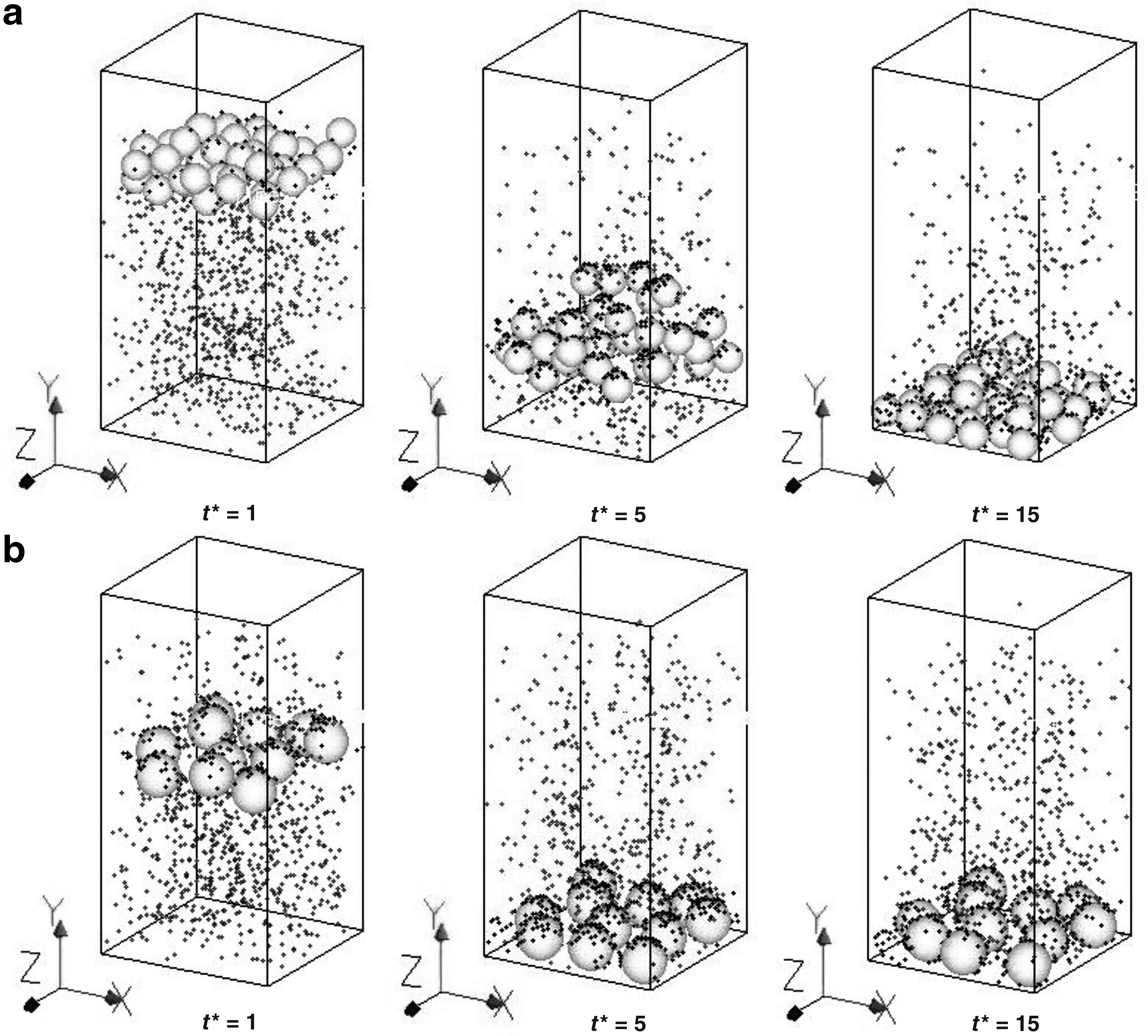
We discuss the influence of the particle diameter ratio R_d=(d_o/d_c) on the sedimentation process. Figure 4 shows the results of snapshots for ϕ^(th)=0.25 and b^(th)=20: Fig. 4a and b are for R_d=15 and 10, respectively. It is noted that a smaller value of the particle diameter implies a more numerous number of large particles in the system for a given set of the values of ϕ^(th) and b^(th).

OPEN IN VIEWER

FIG. 4.

Sedimentation process with adsorption of charged small particles for ϕ^(th)=0.25 and b^(th)=20: (a) R_d=15 and (b) R_d=10.

It is seen from the snapshots that for both cases of the particle diameter, the large particles sediment with adsorbing larger number of small particles at the surface of each large particle with advancing time. Also, it is seen that the large particles with smaller diameter, shown in Fig. 4b, tend to adsorb small particles more significantly as a whole. Even in the case of large particles with smaller diameter, however, relatively large number of small particles remain without being adsorbed and fluctuate in the liquid; small particles that are not adsorbed by large particles require extraordinarily much longer time for sedimentation than large particles, so that they can be regarded as fluctuating in the liquid without sedimentation in the present simulation time. The potential curve shown in Fig. 3c clearly exhibits that adsorbed small particles are unable to dissociate from their large particles because there is a significantly deep energy valley in the net potential curve in a contacting situation of two particles, leading to a strong attractive interaction acting between the large and small particles. We consider the common characteristics of the adsorption process in Fig. 4a and b in more detail. If we see the distribution of the adsorbed small particles on the particle surface, it is seen that the small particles are largely located at the upper side of each particle surface, which is clearly observed in the snapshots at t*=5. On the other hand, the adsorbed small particles at the particle surface at t*=15 are observed to be scattered in the larger area than those at t*=5. This may be explained in the following manner. First, for the following discussion, we have to take into account the fact that the potential curve in Fig. 3c exhibits that the small particles attached at the surface of the large particles do not dissociate from the large particles because a significantly strong attractive interaction acts on these small particles. Moreover, as mentioned above, small particles are assumed to be sufficiently small and therefore they do not sediment but strongly tend to fluctuate in the whole simulation area. During the sedimentation process of large particles, small particles are first adsorbed at the contact point, and these small particles move to the upper areas of the large particles while the large particles are sedimenting. Since a strong attractive interaction acts between large and small particles, it is not possible for adsorbed small particles to dissociate from the large particle. However, random forces still act on these adsorbed particles at the surface of the large particles because random forces arise from the motion of the ambient solvent molecules. If random forces do not act on the small particles, it is reasonable for the adsorbed small particles to stay at the adsorbed point of the surface of the large particle. In the present situation, the movement of the adsorbed small particles is induced by the random force acting on those small particles. Also, we have to take into account the assumption that only the center-to-center interactions are employed between two particles. This implies that there are no friction forces acting on the adsorbed small particles that move along the surface of the large particle due to the random forces. We now discuss why the adsorbed small particles move to the upper areas of the surface of the large particles. The movement of the small particles at the surface arises due to the difference in the inherent sedimentation time scales between the small and the large particles. That is, the adsorbed small particles attempt to sediment together with the large particles, but the large particles inherently sediment much faster than the adsorbed small particles. As already mentioned, the adsorbed small particles cannot dissociate from the large particles due to the electrical interaction and therefore they move to the upper areas of the large particles due to the influence of the random forces, which are clearly seen in Fig. 4a and b at t*=5. After the small particles arrive at the upper areas of the large particles, they will sediment together with the large particles, staying at the upper areas. After the arrival to the bottom wall, the adsorbed small particles in the upper area tend to scatter in the side area of the surface due to the influence of the random forces and the repulsive interaction between the adsorbed particles, which is seen at the snapshots at t*=15, leading to less dense small particles in the snapshots at t*=15 than at t*=5. Large particles sediment faster for R_d=15 (Fig. 4a) than for R_d=10 (Fig. 4b). This is because larger particles have a larger mass and these particles are more significantly influenced by the gravitational force. Equation (38) suggests that the random displacement becomes shorter with increasing diameter of the large particles, which implies that the particle Brownian motion is not sufficiently activated. Hence, the large particles are seen to sediment faster without significantly performing Brownian motion. It is also seen that the large particles in Fig. 4a adsorb much more small particles, per large particle, than in Fig. 4b, but the total number of small particles adsorbed by the large particles is much larger for R_d=10 than that for R_d=15 in the situation of the same input amount (volume) of large particles. From these results, we may derive a conclusion that putting numerous adsorbing particles with smaller diameter into water is more effective for removing the suspended substances or dirty particles if the same input amount of adsorbing agents is used.

Finally, it is noted that large particles become slightly heavier with increasing number of adsorbed small particles, but this effect may not significantly appear in the adsorption performance, because we focus on the large particle diameter ratio such as 10, 15, and 20 in the present simulations and also because the random forces still act on the adsorbed particles. Moreover, it is noted that in the application of the present technique, as already mentioned in the Introduction, the deposited large particles adsorbing small particles will be regularly removed from the surface of the bottom of the lake or pond of interest.

Time change in adsorption rate

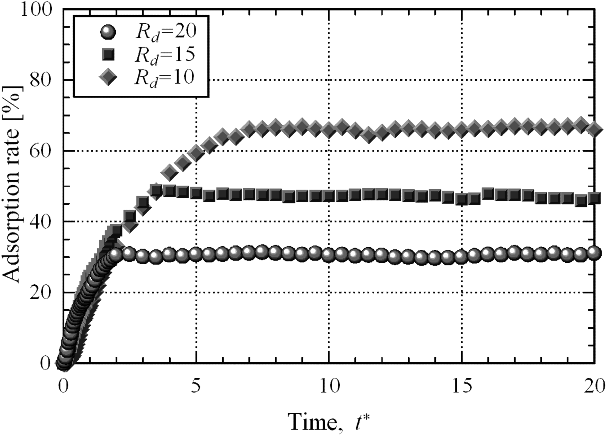
We next make a quantitative discussion by focusing on the time change in the adsorption rate N^(ads)/N_ss, which is the ratio of the number of adsorbed small particles, N^(ads), to the total number of small particles in the system, N_ss. Figure 5 shows how the adsorption rate changes with time for ϕ^(th)=0.25 and b^(th)=20: three curves are plotted for the cases of the particle diameter, R_d=10, 15, and 20. It is seen from these curves that for all the cases of the particle diameter, the adsorption rate increases with advancing time and a more significant performance can be obtained during a longer period for a smaller diameter case: the adsorption rate first exhibits a steep increase, then a gradually slower increase, and finally no increase with advancing time, which is a common feature among the three cases of the diameter. These characteristics of the adsorption rate can be explained in the following lines. The steep curve in the first stage of adsorption corresponds to the adsorption of the surrounding small particles almost freely. Why the adsorption curve gradually becomes gentler with advancing time is that the number of the ambient small particles around large particles gradually decreases in the adsorption process and also the adsorbed particles at the particle surface become an obstacle for other ambient small particles being adsorbed. In the final stage, all the large particles attain to the bottom wall, leading to actually no adsorption performance. The reason why the large particles with smaller diameter can maintain an adsorption performance during a longer period is that such large particles perform the Brownian motion more significantly and therefore remain in the water for a longer time, which yields a higher and longer adsorption performance; an increase in the total surface area of large particles with decreasing diameter may be another factor for providing more opportunity to contact with small particles. A gentle approach to a final adsorption rate for R_d=10 is due to the fact that the Brownian motion induces the large particles to collide with the bottom surface and to repeatedly attach to and detach from the surface; as already mentioned, the specular collision model was used for the boundary condition at the bottom surface.

OPEN IN VIEWER

FIG. 5.

Time variation of the adsorption rate for ϕ^(th)=0.25 and b^(th)=20.

Influence of amount of oppositely charged large particles

Finally we discuss how many large particles we should use to adsorb small particles more efficiently. To do so, we concentrate on the dependence of the adsorption rate on the input amount of large particles. If an extraordinarily large amount of large particles are unnecessarily used, many large particles just sediment to the bottom wall without adsorbing small particles. This leads to a poor performance of adsorption in a commercial meaning. Hence, we here consider the results of the adsorption rate for the various cases of the volumetric fraction ϕ^(th) of large particles under the condition of one set of the particle diameter ratio and the thickness b^(th) of the layer of large particles, (b^(th), R_d)=(20,10); the value of ϕ^(th) was taken as ϕ^(th)=0.10, 0.15, 0.20, 0.25, and 0.30. The other parameters are the same as in the case of R_d=10 in Figs. 5 and 6. Figure 6 shows the time change of the adsorption rate for the various cases of the volumetric fraction of large particles, and Figs. 7–9 show the relationship between the number of adsorbed small particles and the number of the large particles adsorbing such small particles.

OPEN IN VIEWER

FIG. 6.

Time variation of the adsorption rate for R_d=10 and b^(th)=20.

OPEN IN VIEWER

FIG. 7.

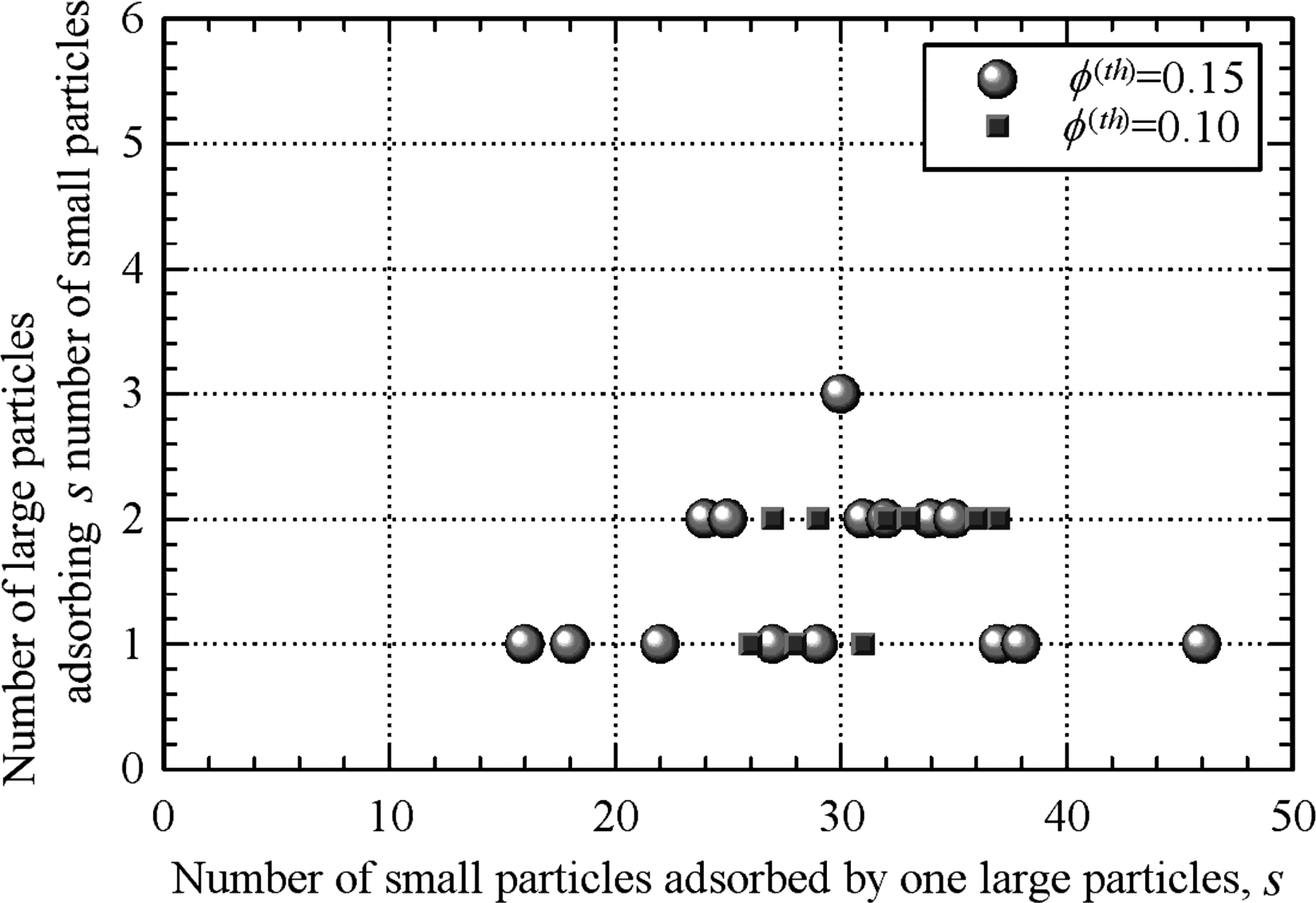
Distribution of number of large particles adsorbing small particles with the number in the abscissa for ϕ^(th)=0.10 and 0.15.

OPEN IN VIEWER

FIG. 8.

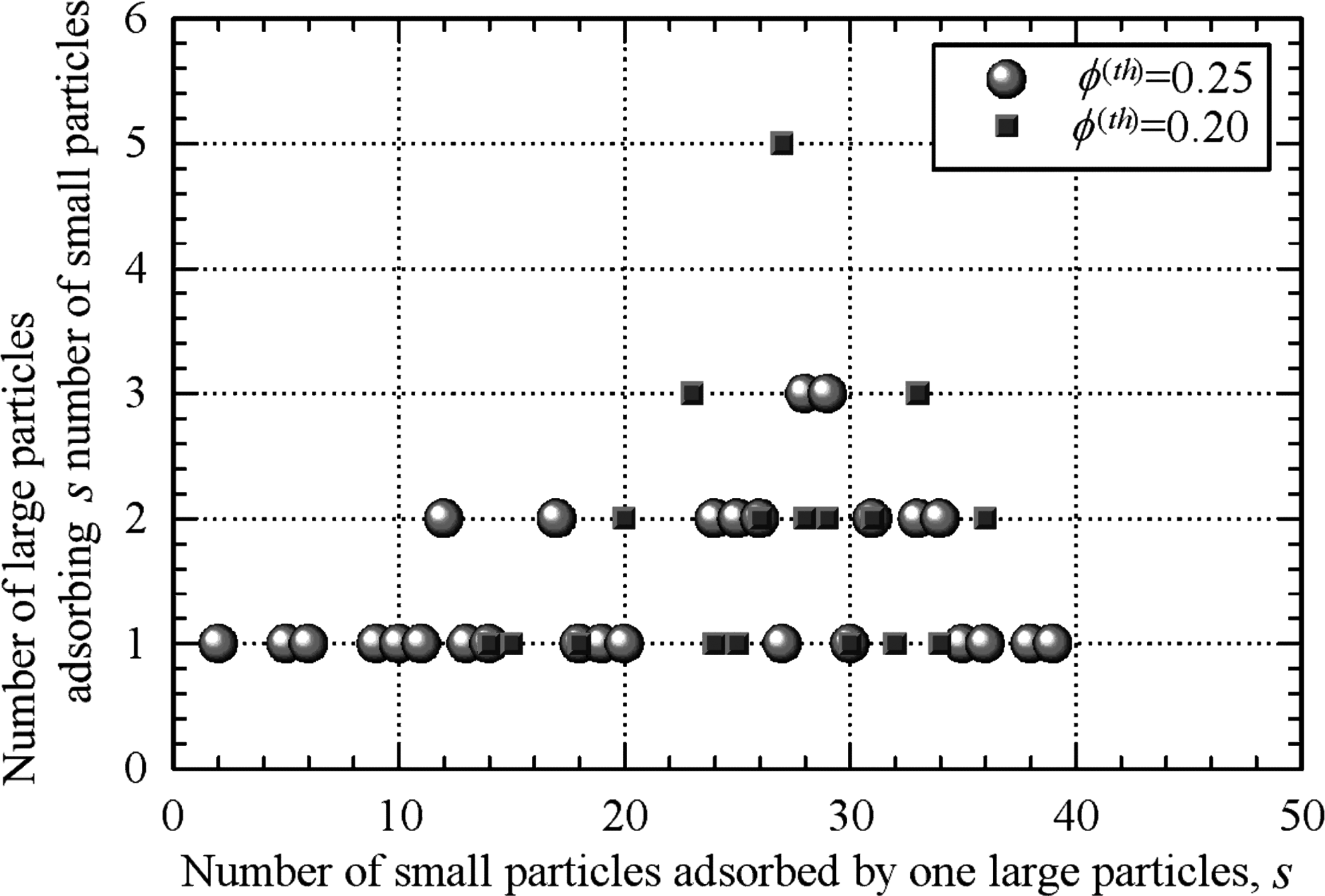
Distribution of number of large particles adsorbing small particles with the number in the abscissa for ϕ^(th)=0.20 and 0.25.

OPEN IN VIEWER

FIG. 9.

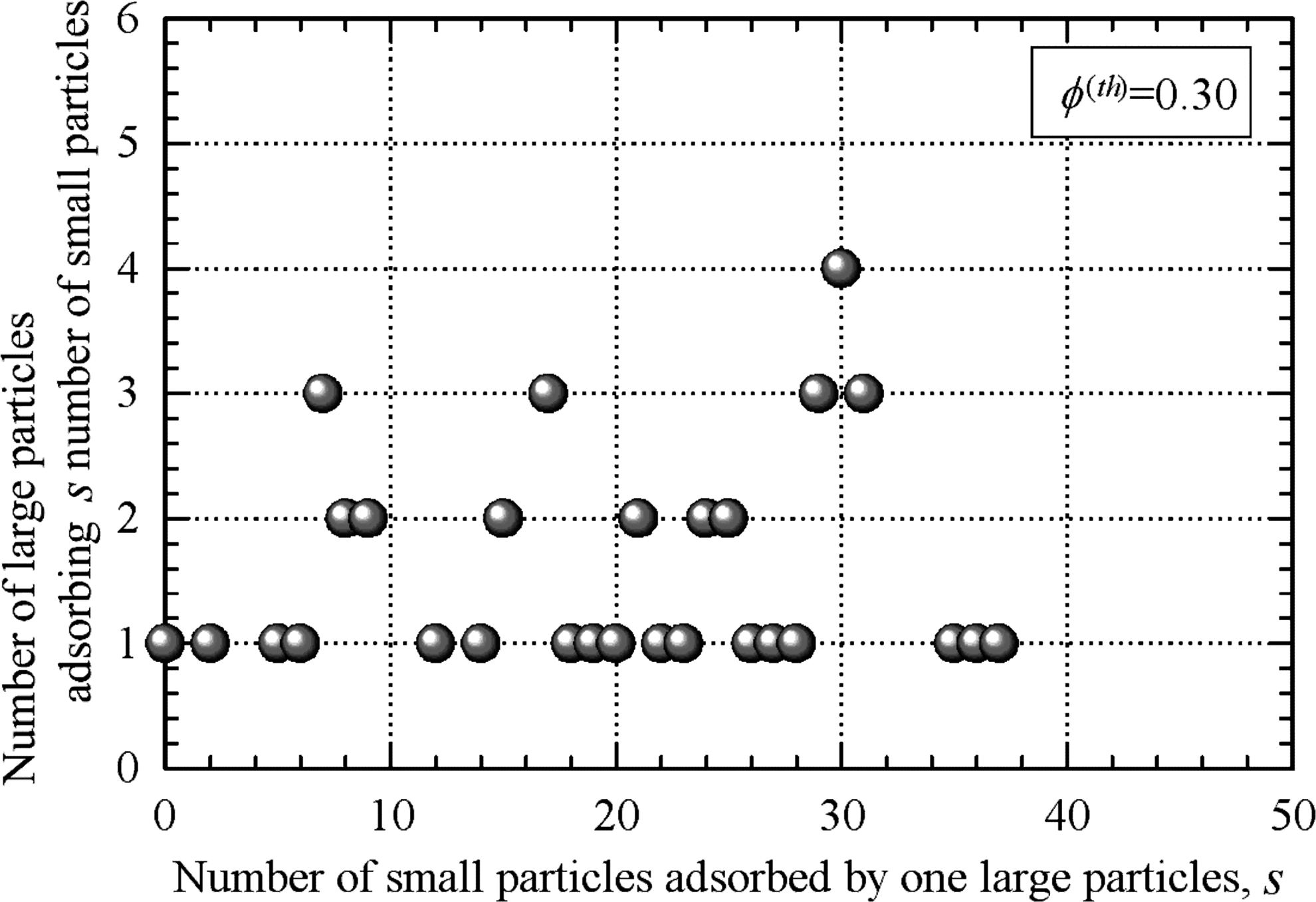
Distribution of number of large particles adsorbing small particles with the number in the abscissa for ϕ^(th)=0.30.

Figure 6 shows the time change in the adsorption rate for the five cases of the volumetric fraction of large particles. It is seen from Fig. 6 that a larger adsorption rate can finally be obtained for a larger volumetric fraction, although the period of the adsorption process functioning is almost independent of the volumetric fraction. This may be a physically reasonable result since the input amount of large particles increases with the volumetric fraction. On the other hand, it is seen that the effect of the increase in the input amount of large particles becomes more inefficient; in other words, the maximum adsorption rate is not proportional to the input amount. This suggests that there is an appropriate input amount of large particles for obtaining the best adsorption performance in a commercial meaning. Therefore, we discuss the adsorption performance. Before that discussion, we consider why the adsorption curve for ϕ^(th)=0.10 slightly decreases after passing the maximum point at time t*≃7. It is noted that this characteristic is not observed for the other cases of the volumetric fraction. Hence, we may understand that in a dilute situation of large particles, there are sufficient possibilities for small particles to be adsorbed in a subtle manner, which implies that small particles may be adsorbed in a noncontact situation that may be made by the already adsorbed small particles at the surface of the large particles. This subtle configuration may come to appear more frequently when a sufficient number of small particles cover the surface of the large particles. These indirectly adsorbed small particles are not strongly combined with the large particles, so that the change in the situation at the surface of the large particles induces the dissociation of the small particles. However, another sophisticated study is necessitated to conclude the reason for the above-mentioned characteristic of the adsorption curve for ϕ^(th)=0.10.

Figures 7–9 show the relationship between the number of adsorbed small particles per large particle, s, and the number of the large particles adsorbing s number of small particles. For the case of small volumetric fractions, shown in Fig. 7, the data are almost plotted in the center and right-side areas, so that each large particle adsorbs many small particles during the sedimentation. This implies that almost all large particles function effectively as an adsorption agent. For the case of relatively large volumetric fractions, shown in Fig. 8, the data are plotted in the center and left-side areas and therefore several large particles that adsorb only a few small particles come to appear in this situation. For the case of a large volumetric fraction, shown in Fig. 9, the number of large particles that adsorb none or only several small particles significantly increases. This implies that even if the input amount of large particles is increased, an adsorption performance cannot significantly be improved; the number of inefficient large particles that do not contribute to the adsorption performance increases. From these results, we understand that there is an optimal input amount of adsorption agents from a commercial point of view.