Artificial Neural Network Approach for Forecasting Nitrogen Oxides Concentrations

Abstract

This article presents the application of feed-forward multilayer perceptron (MP) networks to forecast hourly nitrogen oxides levels 24 h in advance. Input data were meteorological variables, average hourly traffic, and nitrogen oxides hourly levels. The introduction of four periodic components (sine and cosine terms for the daily and weekly cycles) was analyzed to improve the models' prediction powers. Data were measured during 3 years at monitoring stations in Valencia (Spain) in two locations with high traffic density. The models' evaluation criteria were mean absolute error, root mean square error (RMSE), mean absolute percentage error, and correlation coefficient between observations and predictions. Comparisons of MP-based models proved that insertion of four additional seasonal input variables improved the ability of obtaining more accurate predictions, which emphasizes the importance of taking into account seasonal character of nitrogen oxides. When using seasonal components as predictors, root mean square error improves from 20.29 to 19.35 when predicting nitrogen dioxide and from 45.07 to 42.37 when forecasting nitric oxides if the model includes seasonal components at one study location. At the other location, RMSE changes from 23.76 to 23.05 when predicting nitrogen dioxide and from 33.94 to 33.10 for other pollutant's forecasts. Neural networks did not require very exhaustive information about air pollutants, reaction mechanisms, meteorological parameters, or traffic characteristics, and they had the ability of allowing nonlinear and complex relationships between very different predictor variables in an urban environment.

Introduction

Air pollution in urban areas is a worldwide growing problem. Administrations introduce plans and regulations to reduce pollutant emissions. Emission directives establish limit values for concentrations of pollutants with the aim of avoiding, preventing, and reducing the harmful effects on human health and the environment as a whole (Senger, 2000). Modeling temporal variations in the concentration of pollutants is useful when evaluating the effectiveness of these plans. These models allow long- and short-term forecasting of pollution levels. They have to take into account the link between climate and pollutants, which plays an important role in the variability.

Tools to predict pollution levels can be used in different ways. Deterministic and statistical models have been developed for the purpose of forecasting. Deterministic models are not appropriate as prognostic models in coastal zones (Rye, 1995). They are more suitable for extensive areas such as whole regions and large cities. One of the causes of the uncertainty of deterministic models is the lack of sufficient data, as they require precise data from the emission and transportation of pollutants (deriving from traffic) and meteorological conditions. As the complexity of a problem increases, the theoretical understanding decreases due to ill-defined interactions between systems, and statistical approaches are required.

Statistical models are able to establish a relationship between input variables (predictors) and output variables, without detailing the causes and effects of the formation of pollutants. Autoregressive statistical models are often used to analyze the seasonality, trend, and autocorrelation of pollutant variability (Prada-Sanchez et al., 2000; Box et al., 2008), but they are limited by their weakness when modeling nonlinear temporal variations.

Classification and regression trees have also been applied to study the pollutant variability (Ryan, 1995; Gardner and Dorling, 2000). The possible presence of chaotic dynamics in pollutant concentrations allows modeling of nonlinear time series (Kocak et al., 2000). Donnelly et al. (2015) applied a nonparametric kernel regression model to forecast nitrogen dioxide concentrations 48 h in advance, using temporal variations and correlations with meteorology. The model had low computational resources and gave the index of agreement values between 0.74 and 0.94.

During the last two decades, the use of artificial neural networks and, in particular, the application of multilayer perceptron (MP) models have been developed to forecast pollutant concentrations (Gardner and Dorling, 1998). Neural networks have been shown to be effective alternatives to more traditional statistical techniques (Shalkoff, 1992). The neural network models can be trained to approximate virtually any smooth measurable function (Hornik et al., 1989). Unlike other statistical techniques, they make no prior assumptions concerning the data distribution. They can model highly nonlinear functions and can be trained to accurately generalize when presented with new unseen data (Bishop, 1995).

These features of neural networks make them an attractive alternative to developing numerical models and also when choosing between statistical approaches. Ibarra-Berastegi et al. (2008) focused on the prediction of hourly levels up to 8 h ahead for five pollutants at six locations in the area of Bilbao (Spain) using MP. The best performance of these models at the different sensors in the area was obtained for the prediction of nitrogen dioxide (NO₂) 1 h ahead (correlation coefficient between observations and predictions=0.9), and the worse results were observed for the prediction of ozone 8 h ahead.

Caselli et al. (2009) compared the MP and multivariate regression models to predict critical pollution events. The regression models gave less accurate results mostly for 1 day forecasting and failed when fitting spiked high values of pollutant concentrations. Arhami et al. (2013) investigated the combination of artificial neural networks and Monte Carlo simulations to quantify model uncertainty when predicting several pollutants at two urban sampling locations of a developing country. They used meteorological parameters and seasonal components as predictors and validated the models with simulated data. They concluded that this methodology allowed selecting input variables and models' architecture in their study area. The best mean square errors obtained were 18.7 for nitrogen dioxide predictions and 27.5 for nitric oxides.

Elangasinghe et al. (2014) developed an artificial neural network model for predicting nitrogen dioxide concentrations at a site near a major highway in Auckland, New Zealand. They compared models with different inputs (meteorological parameters, hour, day, and month). Their study revealed that carefully choosing of inputs can give more reliable nitrogen dioxide forecasts, but the authors indicated that the inclusion of emission rates might improve the methodology. The artificial neural network model outperformed a linear regression model based on the same input parameters.

The objective of this study is to investigate, for the first time, the capability of the MP method to forecast NO₂ and nitric oxide (NO) concentrations in the Valencia urban area (Spain). The primary goal of the work is to predict concentrations 24 h ahead at two different locations. This forecasting period of 24 h has been selected for practical regulatory reasons; shorter time forecasts are of minimal value for air quality management purposes.

NO₂ and NO are relevant air pollutants in Valencia (European Communities, 2007). They are mainly a consequence of motor vehicle emissions, and industrial pollution plays a smaller part (Ballester et al., 2005). Tenias et al. (1998) reported a significant connection between a 10 μg/m³ increase in the NO₂ level and the relative risk of asthma emergency visits in Valencia. Daily levels of NO₂ in this city are also associated with cardiovascular admissions (Ballester et al., 2001; Ballester et al., 2006).

This pollutant is a precursor of other secondary pollutants that are related to photochemical smog and acid rain. Ambient air NO₂ is, in large part, originated by the oxidation of NO. The link between climate and these pollutants plays an important role on their variability and has to be taken into account when selecting optimal pollutant reduction strategies to avoid exceeding emission directives. In this article, several MP models are designed and compared to establish the most efficient performer as a forecasting tool using meteorological and traffic variables, pollutant concentrations, and seasonal components as predictors.

Materials and Methods

Study area and database

The study area is located in Valencia (Spain). This city has around 1 million inhabitants, mediterranean climatology, and structure. An air pollution network managed by the local government since 1995, measures pollution variables in its urban area. The traffic network of the local municipality measures the number of vehicles circulating every hour at locations close to the pollution monitoring sites. The data used in this work were hourly observations from the air pollution and traffic networks.

The study considers two monitoring stations: Pista Silla and Viveros. Figure 1 presents the map of the study monitoring sites' location. These two stations were selected because several high-pollution episodes were registered to them during the period 2002–2005. The limit value of NO₂ for the protection of human health in a calendar year (averaging period) was exceeded at Pista Silla in 2003–2005. At this site, the highest annual NO₂ mean was observed in 2003.

FIG. 1.

Map of study monitoring sites' locations.

Mass concentrations of nitrogen oxides are determined using the chemiluminescence method. Pollutant concentrations are expressed in μg/m³. The volumes are standardized at a temperature of 293°K and a pressure of 101.3 kPa. The air pollution monitoring site at Pista Silla also measures wind speed (WS, m/s), wind direction (WD, degrees), temperature (T, °C), solar radiation (SR, W/m²), relative humidity (RH, %), and pressure (P, mbar). At Viveros location, WS, WD, T, and SR observations were provided by the National Institute of Meteorology, which manages a meteorological station close to the air pollution station.

The Pista Silla station is in a roadside site located a few meters from a motorway, and Viveros is in an avenue close to the city's center. The distance between them is 2.6 km. Traffic density is high at both sites. The matrix of data (hourly measurements) had 18,339 entries for Pista Silla (years 2003–2005) and 16,221 for Viveros (years 2002–2004), after eliminating rows with missing values. Table 1 shows averages, coefficients of variation, maximum values of pollutants, and meteorological and traffic variables for both stations, during the study period.

Table 1.

Mean, CV, Maximum Values of Pollution, and Meteorological and Traffic Data for the Two Monitoring Stations

Station	Variable	Mean	CV	Maximum
Pista Silla	NO₂	58.8	0.51	249
	NO	52.0	1.14	624
	WS	1.1	0.82	8.6
	WD	187.8	0.57	360
	T	18.7	0.36	38.2
	RH	60.8	0.25	92
	P	1,022.2	0.01	1,044.7
	SR	153.3	1.60	947
	NV	2,945.7	0.57	38,712
Viveros	NO₂	36.72	0.67	238
	NO	19.6	1.93	596
	WS	1.8	0.72	11.9
	WD	168.3	0.69	360
	T	18.9	0.34	38.2
	SR	170	1.53	1,033.3
	NV	1,088.7	0.66	13,456

NO₂ and NO, nitrogen dioxide and nitric oxide are expressed in μg/m³; WS, wind speed in m/s; WD, wind direction in degrees; T, temperature in °C; SR, solar radiation in W/m²; RH, relative humidity in%; P, pressure in mbar; NV, number of vehicles circulating every hour; CV, coefficient of variation.

Factors mainly contributing to NO₂ and NO concentrations are connected with the source activity (e.g., traffic) and periodic variations in nature (e.g., photochemical reactions in the atmosphere). Periodic components are expected in the time series at the week level and in the form of daily variations. Figure 2 represents the average diurnal cycle of NO₂ and NO levels at Pista Silla during the study period. The average weekly cycle at the same station for the two pollutants can be seen in Figure 3. The average traffic strength is also plotted in these diagrams with another scale on the right side. There are differences between hours, with concentration peaks associated with a high traffic density. The daily and weekly variations of the two pollutants depend on the average daily and weekly traffic variations. The same cyclical patterns were observed at the Viveros station.

FIG. 2.

Average diurnal cycles at Pista Silla station.

FIG. 3.

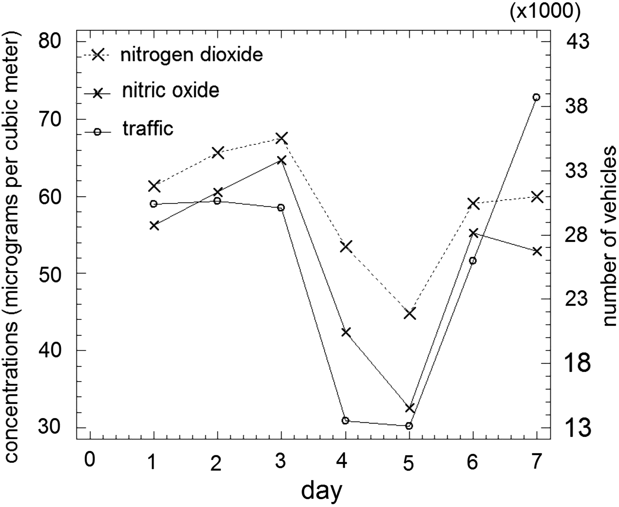
Average weekly cycles at Pista Silla station.

Multilayer perceptrons

The MP models used in this work were composed of three layers of neurons: the input layer, the hidden layer, and the output layer. The models were compared with different number I of predictors X_i or neurons in the input layer. The predictors were pollutant concentrations, meteorological parameters, traffic variables, or seasonal components (sine and cosine terms for the daily and weekly cycles). The models' output Y was the prediction of NO₂ or NO concentrations 24 h in advance; therefore, the number of neurons in the output layer was equal to 1. Table 2 shows the models that were analyzed. The number of neurons H in the hidden layer was determined by experimentation, training the neural networks with values of H from 5 to 30. Greater values of H did not give a better performance.

Table 2.

Models Analyzed

Model	Output variable	Input variables
MP1	(NO₂)_t+24	Meteorology_t, traffic_t, (NO₂)_t
MP2	(NO₂)_t+24	Meteorology_t, traffic_t, Seasonality_t+24, (NO₂)_t
MP3	(NO₂)_t+24	Meteorology_t, traffic_t, (NO₂)_t, NO_t
MP4	(NO₂)_t+24	Meteorology_t, traffic_t, Seasonality_t+24, (NO₂)_t, NO_t
MP5	NO_t+24	Meteorology_t, traffic_t, NO_t
MP6	NO_t+24	Meteorology_t, traffic_t, Seasonality_t+24, NO_t
MP7	NO_t+24	Meteorology_t, traffic_t, NO_t, (NO₂)_t
MP8	NO_t+24	Meteorology_t, traffic_t, Seasonality_t+24, NO_t, (NO₂)_t

MP, multilayer perceptron.

The MP networks were trained with two backpropagation algorithms: the scaled conjugate gradient (SCG) algorithm and the Levenberg–Marquardt (LM) algorithm. It has been proved that both algorithms converge faster and perform better than other backpropagation algorithms (Moller, 1993). The output Y^o can be expressed as follows: \documentclass{aastex}\usepackage{amsbsy}\usepackage{amsfonts}\usepackage{amssymb}\usepackage{bm}\usepackage{mathrsfs}\usepackage{pifont}\usepackage{stmaryrd}\usepackage{textcomp}\usepackage{portland, xspace}\usepackage{amsmath, amsxtra}\pagestyle{empty}\DeclareMathSizes{10}{9}{7}{6}\begin{document} \begin{align*}Y^o = f^o \left( b^o + \sum \limits^H_{j = 1} w_j^o f^h \left( b_j^h + \sum \limits_{i = 1}^I w_{ij}^h X_i \right) \right) \tag{1}\end{align*} \end{document}

where o denotes the elements of the output layer and h indicates the elements of the hidden layer. \documentclass{aastex}\usepackage{amsbsy}\usepackage{amsfonts}\usepackage{amssymb}\usepackage{bm}\usepackage{mathrsfs}\usepackage{pifont}\usepackage{stmaryrd}\usepackage{textcomp}\usepackage{portland, xspace}\usepackage{amsmath, amsxtra}\pagestyle{empty}\DeclareMathSizes{10}{9}{7}{6}\begin{document} $$w_j^o$$ \end{document} is the weight that connects the neuron j of the hidden layer with the neuron of the output layer, and \documentclass{aastex}\usepackage{amsbsy}\usepackage{amsfonts}\usepackage{amssymb}\usepackage{bm}\usepackage{mathrsfs}\usepackage{pifont}\usepackage{stmaryrd}\usepackage{textcomp}\usepackage{portland, xspace}\usepackage{amsmath, amsxtra}\pagestyle{empty}\DeclareMathSizes{10}{9}{7}{6}\begin{document} $$w_{ij}^h$$ \end{document} is the weight that connects the neuron i of the input layer with the neuron j of the hidden layer. b^o is the bias of the neuron of the output layer, and \documentclass{aastex}\usepackage{amsbsy}\usepackage{amsfonts}\usepackage{amssymb}\usepackage{bm}\usepackage{mathrsfs}\usepackage{pifont}\usepackage{stmaryrd}\usepackage{textcomp}\usepackage{portland, xspace}\usepackage{amsmath, amsxtra}\pagestyle{empty}\DeclareMathSizes{10}{9}{7}{6}\begin{document} $$b_j^h$$ \end{document} is the bias of neuron j of the hidden layer. f^o is the transfer function of the neuron of the output layer.

In this work, the linear transfer function has been applied for f^o. f^h is the transfer function of neuron j of the hidden layer. The most widely used f^h are the hyperbolic transfer function (tansig) and the logarithmic sigmoid function (logsig): \documentclass{aastex}\usepackage{amsbsy}\usepackage{amsfonts}\usepackage{amssymb}\usepackage{bm}\usepackage{mathrsfs}\usepackage{pifont}\usepackage{stmaryrd}\usepackage{textcomp}\usepackage{portland, xspace}\usepackage{amsmath, amsxtra}\pagestyle{empty}\DeclareMathSizes{10}{9}{7}{6}\begin{document} \begin{align*}tansig ( x ) = \frac { e^x - e^ { - x } } { e^x + e^ { - x } } \tag { 2 } \end{align*} \end{document} \documentclass{aastex}\usepackage{amsbsy}\usepackage{amsfonts}\usepackage{amssymb}\usepackage{bm}\usepackage{mathrsfs}\usepackage{pifont}\usepackage{stmaryrd}\usepackage{textcomp}\usepackage{portland, xspace}\usepackage{amsmath, amsxtra}\pagestyle{empty}\DeclareMathSizes{10}{9}{7}{6}\begin{document} \begin{align*}logsig ( x ) = \frac { 1 } { 1 + e^ { - x } } \tag { 3 } \end{align*} \end{document}

Figure 4 shows an MP model with I neurons in the input layer, H neurons in the hidden layer, and one neuron in the output layer.

FIG. 4.

Multilayer perceptron (MP) model.

Overtraining does occur when the MP memorizes the patterns introduced to it and it is not capable of identifying new situations. The early stopping technique can be used to avoid this problem (Sarle, 1995). In this technique, the available database is separated into three subsets: the training set, the validation set, and the test set. The training set is used to update the network weights and biases. During the training, the validation set is used to guarantee the generalization capability of the model, and training should stop before the error on the validation set begins to rise. The test set is a new set used to check the generalization of the MP. In this work, the models were trained on data from the first year. Data from the second year were used as the validation set, and observations from the third year are the test data set. The computations were performed with the Neural Network Toolbox of MATLAB.

Evaluation criteria

Four statistical parameters were obtained to compare the performance of the MP models with the test dataset. They are the most used indices to assess the quality of an estimator (Willmott et al., 1985; Gomez-Sanchis et al., 2006). The correlation coefficient r between the forecasted values Y_f and the observations Y quantifies the global description of the model. We computed the root mean square error (RMSE): \documentclass{aastex}\usepackage{amsbsy}\usepackage{amsfonts}\usepackage{amssymb}\usepackage{bm}\usepackage{mathrsfs}\usepackage{pifont}\usepackage{stmaryrd}\usepackage{textcomp}\usepackage{portland, xspace}\usepackage{amsmath, amsxtra}\pagestyle{empty}\DeclareMathSizes{10}{9}{7}{6}\begin{document} \begin{align*}RMSE = \sqrt { \frac { \sum \nolimits_ { i = 1 } ^n ( Y_i - Y_ { fi } ) ^2 } { n } } \tag { 4 } \end{align*} \end{document}

where n is the number of observations in the test data set. The mean absolute error (MAE) also measures how close forecasts are to observations: \documentclass{aastex}\usepackage{amsbsy}\usepackage{amsfonts}\usepackage{amssymb}\usepackage{bm}\usepackage{mathrsfs}\usepackage{pifont}\usepackage{stmaryrd}\usepackage{textcomp}\usepackage{portland, xspace}\usepackage{amsmath, amsxtra}\pagestyle{empty}\DeclareMathSizes{10}{9}{7}{6}\begin{document} \begin{align*}MAE = \frac { \sum \nolimits_ { i = 1 } ^n \mid Y_i - Y_ { fi } \mid } { n } \tag { 5 } \end{align*} \end{document}

An expression of accuracy of predictions as a percentage can be computed with the mean absolute percentage error (MAPE): \documentclass{aastex}\usepackage{amsbsy}\usepackage{amsfonts}\usepackage{amssymb}\usepackage{bm}\usepackage{mathrsfs}\usepackage{pifont}\usepackage{stmaryrd}\usepackage{textcomp}\usepackage{portland, xspace}\usepackage{amsmath, amsxtra}\pagestyle{empty}\DeclareMathSizes{10}{9}{7}{6}\begin{document} \begin{align*}MAPE = \frac { 1 } { n } \sum \limits_ { i = 1 } ^n \bigg | \frac { Y_i - Y_ { fi } } { Y_i } \bigg | \tag { 6 } \end{align*} \end{document}

Results and Discussion

The best performance indices results at the Pista Silla station are shown in Table 3. It contains the best results obtained with the models MP1–MP4 [output (NO₂)_t+24] and the models MP5–MP8 (output NO_t+24). The table indicates the backpropagation algorithm, the transfer function, and the number of neurons in the hidden layer. The comparison of the results indicates that the most accurate predictions of (NO₂)_t+24 at Pista Silla were obtained with the LM algorithm. The MP2 model using the tansig transfer function and this algorithm gives good values of the four evaluation criteria when the number of neurons in the hidden layer is n_h=14. The values of these indices show that the obtained model is a good estimator. The predictors are meteorological parameters, traffic, seasonal components, and (NO₂)_t concentrations.

Table 3.

Best Performance Criteria Results at Pista Silla for Models MP1, MP2, MP3, and MP4 [Output (NO₂)_t+24] and Models MP5, MP6, MP7, and MP8 (Output NO_t+24)

Model	Transfer function	n_h	Learning algorithms	RMSE	MAE	MAPE	R
MP1	Tansig	16	LM	20.29	16.39	0.51	0.59
MP2	Tansig	14	LM	19.35	15.38	0.45	0.63
MP3	Logsig	30	LM	20.48	16.32	0.48	0.56
MP4	Logsig	10	LM	20.49	16.55	0.50	0.65
MP5	Logsig	7	LM	45.07	27.85	1.31	0.61
MP6	Logsig	10	LM	42.37	26.48	1.19	0.66
MP7	Logsig	10	LM	45.26	28.39	1.42	0.59
MP8	Logsig	7	LM	42.57	25.57	1.13	0.66

LM, Levenberg–Marquardt; MAE, mean absolute error; MAPE, mean absolute percentage error; RMSE, root mean square error.

Figure 5 represents predictions with this model corresponding to the first 100 h of the test data set. The period is from 00:00 h on January 1, 2003, to 3:00 h (am) on January 5, 2003. Valencia shows clear seasonal variations, with increasing activity during the coldest months. Nitrogen oxides emissions are higher during times of lower temperatures and also increase with reduced traffic speed, which in Valencia also occurs during winter months when urban locations have a greater density of traffic. The optimal neural network matches actual observations very appropriately and captures the concentrations' peaks and troughs. Figure 6 gives the scatterplot of the data set test predictions versus observations.

FIG. 5.

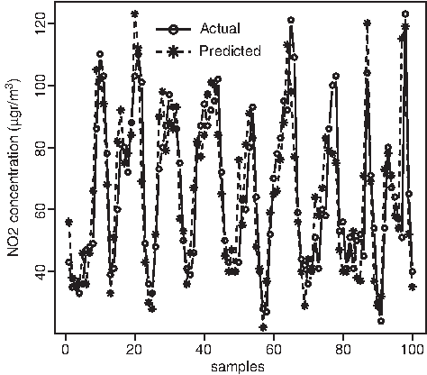
Nitrogen dioxide prediction 24 h in advance in first 100 h of the test data set at Pista Silla. The model is the MP, including (NO₂)_t, meteorology, traffic, and seasonality as predictors, with 14 neurons in the hidden layer, the tansig transfer function, and the Levenberg–Marquardt (LM) backpropagation algorithm. Correlation coefficient r=0.63 and mean absolute error (MAE)=15.38.

FIG. 6.

Scatterplot of nitrogen dioxide predictions 24 h in advance versus observations at Pista Silla. The model is the MP, including (NO₂)_t, meteorology, traffic, and seasonality as predictors, with 14 neurons in the hidden layer, the tansig transfer function, and the LM backpropagation algorithm.

The evaluation of NO_t+24 predictions at Pista Silla is also in Table 3. In this case, the LM algorithm also gives most accurate forecasts. The MP6 model with n_h=10, this algorithm, and the logsig transfer function provided the best value of the RMSE. In this case, the predictors are meteorology, traffic, seasonality, and NO_t concentration. The model MP8 gives better prediction results in terms of MAE and MAPE. This model includes all the potential predictors (Table 2).

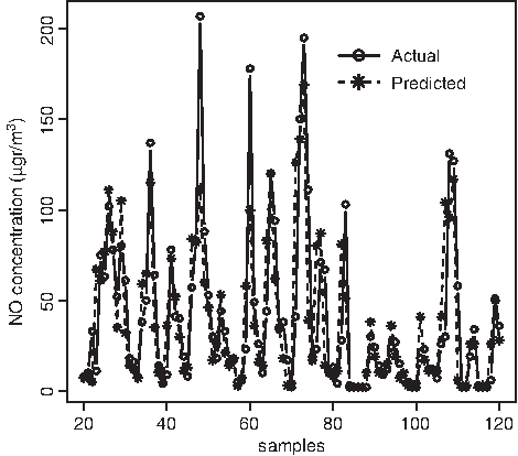
The Figure 7 shows actual and predicted values of NO_t+24 with this model for the first 100 h of the test data set (from 00:00 h on January 1, 2003, to 3:00 h am on January 5, 2003). The neural model fits the observed values correctly. The accuracy of predictions of these models for the two pollutants can be compared using the two adimensional parameters, MAPE and r. MAPE, which computes this accuracy as a percentage, is better for (NO₂)_t+24 (MAPE=0.45) than for NO_t+24 (MAPE=1.13).

FIG. 7.

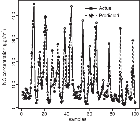
Nitric oxide prediction 24 h in advance in first 100 h of the test data set at Pista Silla. The model is the MP, including NO_t, (NO₂)_t, meteorology, traffic, and seasonality as predictors, with seven neurons in the hidden layer, the logsig transfer function, and the LM backpropagation algorithm. Correlation coefficient r=0.66 and MAE=25.57.

Table 4 shows the best prediction results of the test data set at the Viveros station. Forecast evaluations of (NO₂)_t+24 can be seen in the first four rows (models MP1–MP4). Very similar results were obtained with the two transfer functions. The MP2 model gives the best RMSE result as can be seen in the table, when using the SCG algorithm, the tansig transfer function, and with a number of neurons in the hidden layer n_h=10. The inputs to the neural network are meteorological variables, traffic, seasonal components, and (NO₂)_t levels. Predictions of this model in the first 100 h of the test data set are plotted in Figure 8. The period is from 17:00 h on February 25, 2002 (the first complete record), to 21:00 h on February 28, 2002. The value of the MAPE=0.98 indicates that the fit is less accurate than at Pista Silla, where the MAPE results are smaller with the four models (Table 3).

FIG. 8.

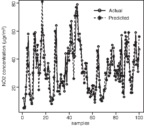
Nitrogen dioxide prediction 24 h in advance in first 100 h of the test data set at Viveros. The model is the MP, including (NO₂)_t, meteorology, seasonal components, and traffic as predictors, with 10 neurons in the hidden layer, the tansig transfer function, and the Scaled Conjugate Gradient backpropagation algorithm. Correlation coefficient r=0.07 and MAE=18.31.

Table 4.

Best Performance Criteria Results at Viveros for Models MP1, MP2, MP3, and MP4 [Output (NO₂)_t+24] and Models MP5, MP6, MP7, and MP8 (Output NO_t+24)

Model	Transfer function	n_h	Learning algorithms	RMSE	MAE	MAPE	R
MP1	Logsig	5	SCG	23.76	18.16	0.93	0.03
MP2	Tansig	10	SCG	23.05	18.31	0.98	0.07
MP3	Logsig	16	SCG	23.28	18.41	0.93	0.15
MP4	Logsig	12	SCG	23.32	18.31	0.91	0.05
MP5	Logsig	5	LM	33.78	19.86	3.52	0.49
MP6	Logsig	16	LM	33.19	19.03	3.16	0.52
MP7	Tansig	10	LM	33.94	19.26	3.20	0.49
MP8	Tansig	10	LM	33.10	19.10	3.32	0.52

SCG, scaled conjugate gradient.

The correlation coefficients between (NO₂)_t+24 observations and predictions are very small in Viveros (Table 4). This indicates that the linear agreement between these two variables is very poor and then the performance of the model MP1–MP4 is worse than at Pista Silla. Figure 5 also shows a closer agreement between observations and forecasts than Figure 8. The model MP4, which includes NO_t as a predictor, has a smaller MAPE value.

Evaluation indices for the predictions of NO_t+24 at Viveros are also in Table 4. The model that provides the best RMSE of NO_t+24 forecasts is the MP8 model at the Viveros station. The transfer function is the tansig, with the LM backpropagation algorithm, and the number of neurons in the hidden layer is n_h=10. Figure 9 shows the time series of NO_t+24 predictions and actual values in the first 100 h with complete data of the test data set at Viveros (the first 20 h had missing records). Predictions are less accurate than at Pista Silla, where the correlation coefficient resulted for this pollutant r=0.66 and the MAPE is equal to 1.13 with this model. At Viveros, these parameters are r=0.52 and MAPE=3.32.

FIG. 9.

Nitric oxide prediction 24 h in advance in first 100 h with complete records of the test dataset at Viveros. The model is the MP, including NO_t, (NO₂)_t, meteorology, traffic, and seasonality as predictors, with 10 neurons in the hidden layer, the tansig transfer function, and the LM backpropagation algorithm. Correlation coefficient r=0.52 and MAE=19.1.

The correlation coefficient is better when predicting NO_t+24 than (NO₂)_t+24 at Viveros, but the agreement between actual and predicted values, expressed as a percentage, is better for (NO₂)_t+24. The MP models might perform worse at Viveros because the nitrogen oxides' temporal variations might depend on other environmental parameters not considered here, such as other meteorology parameters. At the Viveros location, wind speed, wind direction, temperature, and solar radiation observations were used as inputs. At Pista Silla, pressure and relative humidity were also available. Supplementary Tables S1–S6 provide the performance indices for both monitoring sites, and all the MP's parameters.

MP models have the advantages of making no prior assumptions concerning the data distribution. They have also modeled the nonlinear relationships existing between inputs and outputs and have been trained to accurately generalize when presented with new unseen data. They are easy to use and understand compared to other statistical methods. These models can also be applied in other areas with similar air quality problems and meteorological and traffic influences.

Future work will involve their application to forecast other pollutants. However, the MP is a black box learning approach, cannot interpret relationships between inputs and outputs, and cannot deal with uncertainties. There are other linear statistical methods where a greater understanding of the cause and effect can be obtained, but they are not useful in this study, given the highly nonlinear relationships between inputs and outputs. Other approaches such as nonparametric regression models have recently (Donnelly et al., 2015) performed well for air quality prediction in other places. A comparison of MP models with these approaches in the study locations is a promising research area. These models may be a good alternative to the methods used in this work.

Summary

In this work, neural network models and, more particularly, MP models have been developed to forecast nitrogen oxides levels 24 h in advance. This forecasting period was selected because the shorter time forecasts are of minimal value for air quality management purposes. Management of control and public warning strategies for nitrogen oxides levels requires accurate forecasts of the concentration of these pollutants and their dependence on meteorological and traffic variables.

The MP performed better when predicting nitric oxide at the study locations, if the models included daily and weekly seasonal components. These components were introduced with four additional input variables sin (2πh/24), cos (2πh/24), sin (2πd/7), and cos (2πd/7), h=1, 2,…, 24, d=1, 2,…, 7. In one of the monitoring stations (Pista Silla), the best forecast of nitrogen dioxide was obtained when including as input variables, meteorology, traffic, seasonality, and (NO₂)_t level. At the other site (Viveros), the introduction of seasonality improves the performance of the MP when predicting nitrogen dioxide in terms of the RMSE.

The relative importance of meteorological and vehicle emission variables on surface nitrogen oxides predictions is of great interest to establish the legislative measures that permit to reduce their levels. Models with different architectures have been considered. They have allowed predicting nitrogen oxides concentrations with accuracy. Mechanisms involved in nitrogen oxides concentration are complex and nonlinear. Neural networks do not require very exhaustive information about air pollutants, reaction mechanisms, meteorological parameters, or traffic flow. They also have the advantage of allowing nonlinear relationships between very different inputs or predictor variables.

The application of the models could be extended to forecast the other pollutant's hourly levels in the study area. The predictor variables of this work represent an excellent starting point, but models that consider other inputs should be taken into account for future work. The results support other studies done in other parts of the world using artificial neural network (ANN) techniques (Ibarra-Berastegi et al., 2008, Elangasinghe et al., 2014).

It is the first time that this methodology is applied to the Valencia urban area to predict nitrogen oxides concentrations. If the models were to be used as operational air quality forecast models, forecast traffic data would also be required. This forecast traffic could be obtained by applying ANN using seasonal components as inputs. Forecast traffic values can be used as models' inputs and might improve their performance. A comparison of the models using representative values and forecast traffic data would be useful to evaluate their effects. Future research will also focus on the development of other neural network models for atmospheric pollutant's prediction. Finally, the methodology developed in this study could also be applied in different areas with similar air quality problems and meteorological and traffic influences.

Footnotes

Acknowledgment

The author is indebted to the referees for their constructive comments, which have contributed to improving this article.

Author Disclosure Statement

No competing financial interests exist.

References

Arhami

, Kamali

, and Rajabi

M.M.

(2013). Predicting hourly air pollutant levels using artificial networks coupled with uncertainty analysis by Monte Carlo simulations. Environ. Sci. Pollut. Res., 5, 4777.

Ballester

, Iñíguez

, and García

(2005). ENHIS-1 Project: WP5 Health Impact Assessment. Local City Report Valencia. Available at: www.apheis.org/CityReports2005/Valencia.pdf. (accessed April 2006 ).

Ballester

, Rodríguez

, Iñíguez

, Sáez

, Daponte

, et al. (2006). Air pollution and cardiovascular admissions association in Spain: Result within the EMECAS project. J. Epidemiol. Community Health, 60, 328.

Ballester

, Tenias

J.M.

, and Pérez-Hoyos

(2001). Air pollution and emergency hospital admissions for cardiovascular diseases in Valencia, Spain. J. Epidemiol. Community Health, 55, 57.

Bishop

C.M.

(1995). Neural Networks for Pattern Recognition. Oxford, UK: Claredon Press.

Box

G.E.P.

, Jenkins

G.M.

, and Reinsel

G.G.

(2008). Time Series Analysis. Forecasting and Control, 4th edition. New Jersey: John Wiley & Sons.

Caselli

, Trizio

, De Gennaro

, and Ielpo

(2009). A simple feedforward neural network for the PM₁₀ forecasting: Comparison with a radial basis function networks and a multivariate linear regression model. Water Air Soil Pollut. 201, 365.

Donnelly

, Misstear

, and Broderick

(2015). Real time air quality forecasting using integrated parametric and non-parametric regression techniques. Atmos. Environ., 103, 53.

Elangasinghe

M.A.

, Singhal

, Dirks

K.N.

, and Salmond

J.A.

(2014). Development of an ANN-based air pollution forecasting system with explicit knowledge through sensitivity analysis. Atmos. Pollut. Res., 5, 696.

10.

European Communities. (2007). Europe's Environment: The Fourth Assessment. Luxembourg: European Environment Agency, Office for Official Publications of the European Community.

11.

Gardner

M.W.

, and Dorling

S.R.

(1998). Artificial neural networks (the multilayer perceptron)—a review of applications in the atmospheric sciences. Atmos. Environ., 32, 2627.

12.

Gardner

M.W.

, and Dorling

S.R.

(2000). Statistical surface ozone models: An improved methodology to account for non-linear behaviour. Atmos. Environ., 34, 21.

13.

Gomez-Sanchis

, Martin-Guerrero

J.D.

, Soria-Olivas

, Vila-Francés

, Carrasco

J.L.

, and del Valle-Tascón

(2006). Neural networks for analysing the relevance of input variables in the prediction of tropospheric ozone concentration. Atmos. Environ., 40, 6173.

14.

Hornik

, Stinchcombe

, and White

(1989). Multilayer feedforward networks are universal approximators. Neural Net., 2, 359.

15.

Ibarra-Berastegi

, Elias

, Barona

, Saenz

, Ezcurra

, and Diaz de Argandoña

(2008). From diagnosis to prognosis for forecasting air pollution using neural networks: Air pollution monitoring in Bilbao. Environ. Modell. Softw., 23, 622.

16.

Kocak

, Saylan

, and Sen

(2000). Nonlinear times series prediction of ozone concentration in Istanbul. Atmos. Environ., 34, 1267.

17.

Moller

M.F.

(1993). A scaled conjugate gradient algorithm for fast supervised learning. Neural. Net., 6, 525.

18.

Prada-Sanchez

J.M.

, Febrero-Bande

, Cotos-Yanez

, Gonzalez-Manteiga

, Bermudez-Cela

, and Lucas-Dominguez

(2000). Prediction of SO₂ pollution incident near a power station using partially linear models and an historical matrix of predictor-response vectors. Environmetrics, 11, 209.

19.

Ryan

W.F.

(1995). Forecasting ozone episodes in the Baltimore metropolitan area. Atmos. Environ., 29, 2387.

20.

Rye

P.J.

(1995). Modelling photochemical smog in the Perth region. Math. Comput. Model., 21, 111.

21.

Sarle

W.S.

(1995). Stopped training and other remedies for overfitting. Proceedings of the 27th Symposium on the Interface. Fairfax, VA.

22.

Senger

S.U.

(2000). Estimation of the reduction of the concentration of air pollutants until the year 2010 in relation to the UN ECEE Göteborg protocol dated 1. December 1999. Umweltwiss. Schadst. Forsch., 12, 152.

23.

Shalkoff

(1992). Pattern Recognition: Statistical Structural and Neural Approaches. New York: John Wiley & Sons.

24.

Tenias

J.M.

, Ballester

, and Rivera

M.L.

(1998). Association between hospital medical emergency visits for asthma and air pollution in Valencia, Spain. Occup. Environ. Med., 55, 541.

25.

Willmott

, Ackleson

, Davis

, Feddema

, Klink

, Legates

, O'Donnell

, and Rowe

(1985). Statistics for the evaluation and comparison of models. J. Geophys. Res., 90, 8995.

Supplementary Material

Please find the following supplemental material available below.

For Open Access articles published under a Creative Commons License, all supplemental material carries the same license as the article it is associated with.

For non-Open Access articles published, all supplemental material carries a non-exclusive license, and permission requests for re-use of supplemental material or any part of supplemental material shall be sent directly to the copyright owner as specified in the copyright notice associated with the article.

0.00 MB

0.06 MB