Surfactant-enhanced aquifer remediation (SEAR) is an efficient way for clearing dense nonaqueous phase liquids (DNAPLs) which may result in serious environment and health threats. To limit the high cost of SEAR, simulation optimization techniques are generally applied to ensure that an optimal remediation strategy is achieved. Furthermore, surrogate model techniques have been widely used to reduce the high computational burden associated with these processes. However, previous research rarely involved comparison of different surrogate models for multiphase flow numerical simulation models. In this regard, we conducted a comparative analysis to select the optimal modeling technique and parameter optimization algorithm for surrogate models in DNAPL-contaminated aquifer remediation strategy optimization problems. Latin hypercube sampling method was used to collect data in the feasible region of input variables. Surrogate models were developed using radial basis function artificial neural network, Kriging, and support vector regression. Genetic algorithm, self-adaptive particle swarm optimization (PSO), and self-adaptive PSO based on simulated annealing (SA) were applied to optimize the parameters of the surrogate model. Results showed that the optimal surrogate model was Kriging model with the parameters obtained by self-adaptive PSO based on SA. Relative errors of the contaminant removal rates between the optimal surrogate model and simulation model for 100 validation samples were lower than 3.5%, clearly confirming the optimal performance of the proposed model. Finally, computation of run time enabled us to conclude that the surrogate model presented in this article was capable of considerably reducing computational burden of simulation optimization processes.
Introduction
Liquid organics, such as chlorinated solvents and petroleum hydrocarbons, have been the critical materials in industrial production since the early 20th century. However, leakages and spills of these chemicals have resulted in serious environmental and health hazards around the world (Fernandez-Garcia et al., 2012). These water-immiscible liquid organic contaminants are generally known as nonaqueous phase liquids (NAPLs). Dense nonaqueous phase liquids (DNAPLs), with densities greater than water, have the characteristics of low solubility, high toxicity, high interfacial tension, and a high tendency to sink below the water (Qin et al., 2007). Several conventional remediation techniques (e.g., pump and treat, vapor extraction, and in situ bioremediation) are commonly unsuccessful or have limited effects on the treatment of DNAPL-contaminated soils/groundwater systems.
Surfactant flushing technology, which is also known as surfactant-enhanced aquifer remediation (SEAR), is a form of chemical enhancement for pump and treats technology. It is capable of increasing the remediation efficiency of the pump and treats technique significantly by enhancing the solubility and mobility of DNAPLs in the aqueous phase (Liu, 2005). However, the surfactants are costly, and this immediately adds to the high cost of SEAR. Thus, the selection of an optimal strategy to increase the remediation efficiency and reduce the remediation cost simultaneously is critical.
Simulation optimization techniques are known to be effective tools for solving such type of problems. Hence, we decided to construct a simulation optimization model with remediation cost minimization at a certain contaminant removal rate as the objective function. The simulation model is embedded in the optimization model as a constraint condition for describing the input/output relationship of system. The input is remediation strategy, and the output is corresponding contaminant removal rate. Multiphase flow simulation modeling has been used by a number of researchers to improve the understanding of the transport mechanisms of NAPLs and identify cost-effective cleanup actions.
Delshad et al. (1996) advanced a three-dimensional multicomponent multiphase compositional finite-difference simulator for analyzing the surfactant-enhanced remediation of aquifers contaminated by NAPLs (UTCHEM). The model they used was originally developed for simulating surfactant-enhanced oil recovery and was adapted for SEAR modeling. Benner et al. (2002) analyzed the factors affecting air sparging remediation systems based on field data and a multiphase simulation model. Liu (2005) developed a multicomponent multiphase numerical model for simulating surfactant-enhanced groundwater remediation and applied it to a tetrachloroethylene (PCE)-contaminated site. Rahbeh and Mohtar (2006) applied multiphase transport models to field remediation by using air sparging and soil vapor extraction.
However, repeatedly invoking a numerical simulation model to resolve the problem is computationally burdensome and limits the applicability of the simulation optimization modeling of SEAR at DNAPL-contaminated sites. The emerging surrogate model is, therefore, of huge potential for addressing this shortcoming. Computational burden will be obviously reduced by replacing the numerical model with an efficient surrogate model (Sreekanth and Datta, 2010). Thus, the most crucial issue of concern is the approximation accuracy of the surrogate model as this would greatly influence the ability of simulation optimization model to perform satisfactorily.
A surrogate model is an approximation model with a similar input/output relationship as the simulation model. Many surrogate model techniques have been applied to groundwater remediation optimization problems. For example, He et al. (2008) replaced numerical models with polynomial regression models when remediating contaminated groundwater systems, whereas Luo et al. (2013) used a radial basis function artificial neural network (RBFANN) building a surrogate model to approximate a DNAPL-contaminated aquifer multiphase flow numerical simulation model. Lu et al. (2013) considerably raised the approximation accuracy of the surrogate model by implementing the Kriging algorithm.
These surrogate models are all able to greatly reduce the large computational load caused by the direct invocation of simulation model in the process of solving optimization model. However, these models are noted for their disparities in terms of their applicability and approximation accuracy for solving solute migration and transformation problems caused by DNAPL pollution. Thus, other methods, such as support vector regression (SVR), should be introduced for selection purposes.
Except for the modeling method, parameter identification is another element that severely impacts the approximation accuracy of surrogate model. As a significant task in itself, parameter optimization has increasingly attracted attention and has developed in many areas. Chiu et al. (2012) used genetic algorithm (GA) to conduct parameter optimization for the fabrication of microlens arrays. Li et al. (2014) adopted GA to optimize parameters for machining optical parts of difficult-to-cut materials. Wang and Huang (2014) implemented particle swarm optimization (PSO) to estimate the mixture of two Weibull parameters with censored data. Manoochehri and Kolahan (2014) integrated artificial neural network and simulated annealing (SA) algorithm to optimize deep drawing process parameters. However, previous efforts to optimize the parameters of surrogate models for DNAPL-contaminated aquifer multiphase flow numerical simulation models are extremely rare.
As an extension of previous studies, the present research selected a more appropriate surrogate model after comparing three advanced surrogate model-building techniques and sought a parameter optimization algorithm capable of searching for the global optimal parameters of the surrogate model at a high convergence speed. This combination is effective in reducing residuals between the surrogate model and simulation model. Naturally, the identification of an optimal surfactant-enhanced aquifer remediation strategy for DNAPL-contaminated sites based on the surrogate model would be more reliable.
The present study was conducted to: (1) use the latin hypercube sampling (LHS) method to derive an input/output dataset for a multiphase flow simulation model; (2) build surrogate models of the multiphase flow simulation model using RBFANN, SVR, and Kriging methods, then evaluate and compare the performance of surrogate models; (3) carry out parameter optimization of the selected surrogate model using GA, self-adaptive PSO, and self-adaptive PSO based on SA, then analyze the optimizing effects; and (4) test the forecasting accuracy of the optimal surrogate model with the optimized parameters.
Methodology
Radial basis function artificial neural network
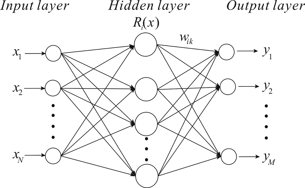
RBFANN is a three-layered feed forward neural network, which consists of an input layer, hidden layer, and output layer, and uses radial basis functions as activation functions. It has been very effective and covers a wide range of applications because of its fast convergence and high stability compared with some other methods (Kegl et al., 2000; Moradkhani et al., 2004).
The structure of RBFANN is shown in Fig. 1. A nonlinear transformation from x to Ri(x) occurs in the hidden layer through a radial basis activation function, whereas the transformation from Ri(x) to yk is linear (Shen et al., 2010). Among the common radial basis functions, the Gaussian function is most widely used. Thus, the output of the neurons in the RBFANN hidden layer is expressed as follows:
\documentclass{aastex}\usepackage{amsbsy}\usepackage{amsfonts}\usepackage{amssymb}\usepackage{bm}\usepackage{yhmath, upgreek}\usepackage{mathrsfs}\usepackage{pifont}\usepackage{stmaryrd}\usepackage{textcomp}\usepackage{portland, xspace}\usepackage{amsmath, amsxtra}\pagestyle{empty}\DeclareMathSizes{10}{9}{7}{6}\begin{document}
\begin{align*}R_i ( { \bf { x } } ) = \phi ( \parallel { \bf { x - c } } _ { \rm i } \parallel ) = \exp \left[ - \frac { \parallel { \bf { x - c } } _i \parallel^2 } { 2 \sigma_i^2 } \right] \tag { 1 } \end{align*}
\end{document}
Structure of radial basis function artificial neural network.
where x is an N-dimensional input vector; ci (i = 1, 2,…, L), which is also an N-dimensional vector, is the center associated with the ith neuron in the radial basis function hidden layer, L is the number of hidden units; σi is the ith radial bias function width parameter; and ∥x − ci∥ is the norm of x − ci. As ∥x − ci∥ increases, Ri(x) rapidly attenuates to zero.
The outputs of the kth neuron in the RBFANN output layer are linear combinations of the hidden layer neuron outputs as follows:
\documentclass{aastex}\usepackage{amsbsy}\usepackage{amsfonts}\usepackage{amssymb}\usepackage{bm}\usepackage{yhmath, upgreek}\usepackage{mathrsfs}\usepackage{pifont}\usepackage{stmaryrd}\usepackage{textcomp}\usepackage{portland, xspace}\usepackage{amsmath, amsxtra}\pagestyle{empty}\DeclareMathSizes{10}{9}{7}{6}\begin{document}
\begin{align*}y_k = \mathop\sum\limits_{i = 1}^{L} w_{ki} R_i ( {\bf x}) - \theta_k \ ( k = 1,2, \ldots , M ) \tag{2}\end{align*}
\end{document}
where wki is the connecting weight from the ith hidden layer neuron to the kth output layer and θk is the threshold value of the kth output layer neuron.
The training of RBFANN occurs in two stages (Boyd, 2010; Navarro et al., 2011):
(1) Use unsupervised algorithms to train the center vectors ci and radial bias function width parameters σi. k-Means clustering algorithm is commonly used (Luengo et al., 2010; Regis, 2011). First, choose several objects among the training samples as initial center vectors ci(0) (i = 1, 2,…, L). Then, distribute the training samples to clusters according to their Euclidean distance with the clustering centers ci(0) and calculate the mean value of each cluster as new clustering center. Repeat the steps until the center vectors stabilize. Meanwhile, σi can be determined.
(2) Use a least squares method for calibrating the connection weights wki from the hidden layer to the output layer. Approximate the network output to the target output by constantly adjusting the connection weights, to eventually make the network convergent.
Kriging
The Kriging method was presented by the French geographical mathematician Matheron and a South African mining engineer named Krige in the 1960s. Sacks et al. (1989) first applied the Kriging method to build a surrogate model. From then on, Kriging became a pervasive surrogate model technique.
The Kriging method was denoted as the sum of two components: the linear model and a systematic departure (Lu et al., 2013). The basic formulation can be expressed as follows:
\documentclass{aastex}\usepackage{amsbsy}\usepackage{amsfonts}\usepackage{amssymb}\usepackage{bm}\usepackage{yhmath, upgreek}\usepackage{mathrsfs}\usepackage{pifont}\usepackage{stmaryrd}\usepackage{textcomp}\usepackage{portland, xspace}\usepackage{amsmath, amsxtra}\pagestyle{empty}\DeclareMathSizes{10}{9}{7}{6}\begin{document}
\begin{align*}
y \left( { \bf{x}} \right) = {{ \bf{f}}^T} \left( { \bf{x}}
\right) { \boldsymbol{\upbeta}} + Z \left( { \bf{x}} \right) =
\mathop \sum \limits_{j = 1}^k {{f_j}} \left( { \bf{x}} \right) {
\beta _j} + Z \left( { \bf{x}} \right) \tag{3}\end{align*}
\end{document}
where \documentclass{aastex}\usepackage{amsbsy}\usepackage{amsfonts}\usepackage{amssymb}\usepackage{bm}\usepackage{yhmath, upgreek}\usepackage{mathrsfs}\usepackage{pifont}\usepackage{stmaryrd}\usepackage{textcomp}\usepackage{portland, xspace}\usepackage{amsmath, amsxtra}\pagestyle{empty}\DeclareMathSizes{10}{9}{7}{6}\begin{document}
$${ \bf{f}} \left( { \bf{x}} \right) = { \left[ {{f_1} \left( {
\bf{x}} \right) , {f_2} \left( { \bf{x}} \right) , \ldots , {f_k}
\left( { \bf{x}} \right) } \right] ^T}$$
\end{document} are determinate regression functions, and \documentclass{aastex}\usepackage{amsbsy}\usepackage{amsfonts}\usepackage{amssymb}\usepackage{bm}\usepackage{yhmath, upgreek}\usepackage{mathrsfs}\usepackage{pifont}\usepackage{stmaryrd}\usepackage{textcomp}\usepackage{portland, xspace}\usepackage{amsmath, amsxtra}\pagestyle{empty}\DeclareMathSizes{10}{9}{7}{6}\begin{document}
$$ \boldsymbol{\upbeta} = (\beta_1 , \beta_2 , \ldots \beta_k) ^
T$$
\end{document} denotes the matrix of regression coefficients to be estimated from the training samples. Z(x) is a local deviation from the regression model with a mean of zero, a variance of \documentclass{aastex}\usepackage{amsbsy}\usepackage{amsfonts}\usepackage{amssymb}\usepackage{bm}\usepackage{yhmath, upgreek}\usepackage{mathrsfs}\usepackage{pifont}\usepackage{stmaryrd}\usepackage{textcomp}\usepackage{portland, xspace}\usepackage{amsmath, amsxtra}\pagestyle{empty}\DeclareMathSizes{10}{9}{7}{6}\begin{document}
$$\sigma _Z^2$$
\end{document}, and nonzero covariance.
The correlation function of N-dimensional vectors u and v is determined by the distance between u and v rather than their sites:
\documentclass{aastex}\usepackage{amsbsy}\usepackage{amsfonts}\usepackage{amssymb}\usepackage{bm}\usepackage{yhmath, upgreek}\usepackage{mathrsfs}\usepackage{pifont}\usepackage{stmaryrd}\usepackage{textcomp}\usepackage{portland, xspace}\usepackage{amsmath, amsxtra}\pagestyle{empty}\DeclareMathSizes{10}{9}{7}{6}\begin{document}
\begin{align*}
R \left( {{ \bf{u}} , { \bf{v}}} \right) = \exp \left( {- {{
\mathop \sum \limits_{i = 1}^n {{ \alpha _i} \,\left|{{u_i} -
{v_i}} \right| } }^2}} \right) \tag{4}
\end{align*}
\end{document}
where αi are uncertain parameters to be optimized, ui and vi are the ith elements of u and v.
where r is the relevance vector of x and samples P: \documentclass{aastex}\usepackage{amsbsy}\usepackage{amsfonts}\usepackage{amssymb}\usepackage{bm}\usepackage{yhmath, upgreek}\usepackage{mathrsfs}\usepackage{pifont}\usepackage{stmaryrd}\usepackage{textcomp}\usepackage{portland, xspace}\usepackage{amsmath, amsxtra}\pagestyle{empty}\DeclareMathSizes{10}{9}{7}{6}\begin{document}
$${ \bf{r}} \left( { \bf{x}} \right) = { \left[ {R \left( {{ \bf{x}} , {{ \bf{p}}_{ \bf{1}}}} \right) , R \left( {{ \bf{x}} , {{ \bf{p}}_{ \bf{2}}}} \right) , \ldots , R \left( {{ \bf{x}} , {{ \bf{p}}_{ \bf{m}}}} \right) } \right] ^T}$$
\end{document}, and F is the response column vector of samples: \documentclass{aastex}\usepackage{amsbsy}\usepackage{amsfonts}\usepackage{amssymb}\usepackage{bm}\usepackage{yhmath, upgreek}\usepackage{mathrsfs}\usepackage{pifont}\usepackage{stmaryrd}\usepackage{textcomp}\usepackage{portland, xspace}\usepackage{amsmath, amsxtra}\pagestyle{empty}\DeclareMathSizes{10}{9}{7}{6}\begin{document}
$${ \bf{F}} = { \left[ {{{ \bf{f}}^T} \left( {{{ \bf{p}}_{ \bf{1}}}} \right) , {{ \bf{f}}^T} \left( {{{ \bf{p}}_{ \bf{2}}}} \right) , \ldots , {{ \bf{f}}^T} \left( {{{ \bf{p}}_{ \bf{m}}}} \right) } \right] ^T}$$
\end{document}.
R is the relevance matrix of samples:
\documentclass{aastex}\usepackage{amsbsy}\usepackage{amsfonts}\usepackage{amssymb}\usepackage{bm}\usepackage{yhmath, upgreek}\usepackage{mathrsfs}\usepackage{pifont}\usepackage{stmaryrd}\usepackage{textcomp}\usepackage{portland, xspace}\usepackage{amsmath, amsxtra}\pagestyle{empty}\DeclareMathSizes{10}{9}{7}{6}\begin{document}
\begin{align*}{ \bf{R}} = \left[ \begin{matrix} R \left( {{{ \bf{p}}_{ \bf{1}}} , {{ \bf{p}}_{ \bf{1}}}} \right) & \cdots & R \left( {{{ \bf{p}}_{ \bf{1}}} , {{ \bf{p}}_{ \bf{m}}}} \right) \hfill \\ \vdots & \cdots & \qquad\vdots \hfill \\ R \left( {{{ \bf{p}}_{ \bf{m}}} , {{ \bf{p}}_{ \bf{1}}}} \right) & \cdots & R \left( {{{ \bf{p}}_{ \bf{m}}} , {{ \bf{p}}_{ \bf{m}}}} \right) \hfill \\\end{matrix} \right] \tag{6}\end{align*}
\end{document}
\documentclass{aastex}\usepackage{amsbsy}\usepackage{amsfonts}\usepackage{amssymb}\usepackage{bm}\usepackage{yhmath, upgreek}\usepackage{mathrsfs}\usepackage{pifont}\usepackage{stmaryrd}\usepackage{textcomp}\usepackage{portland, xspace}\usepackage{amsmath, amsxtra}\pagestyle{empty}\DeclareMathSizes{10}{9}{7}{6}\begin{document}
$$\hat{\boldsymbol{\upbeta}}$$
\end{document} is the estimation of \documentclass{aastex}\usepackage{amsbsy}\usepackage{amsfonts}\usepackage{amssymb}\usepackage{bm}\usepackage{yhmath, upgreek}\usepackage{mathrsfs}\usepackage{pifont}\usepackage{stmaryrd}\usepackage{textcomp}\usepackage{portland, xspace}\usepackage{amsmath, amsxtra}\pagestyle{empty}\DeclareMathSizes{10}{9}{7}{6}\begin{document}
$${\boldsymbol{\upbeta}}$$
\end{document} and can be obtained by the generalized least squares method:
\documentclass{aastex}\usepackage{amsbsy}\usepackage{amsfonts}\usepackage{amssymb}\usepackage{bm}\usepackage{yhmath, upgreek}\usepackage{mathrsfs}\usepackage{pifont}\usepackage{stmaryrd}\usepackage{textcomp}\usepackage{portland, xspace}\usepackage{amsmath, amsxtra}\pagestyle{empty}\DeclareMathSizes{10}{9}{7}{6}\begin{document}
\begin{align*}
\hat{\boldsymbol{\upbeta}} = { \frac{{{\bf { F } } ^T } { { \bf {
R } } ^ { - 1 } } { \bf { Q } } } { { { \bf { F } } ^T } { { \bf
{ R } } ^ { - 1 } } { \bf { F } } } } \tag { 7 }
\end{align*}
\end{document}
Support vector regression
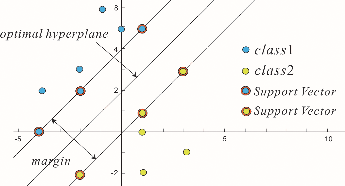
Support vector machine (SVM) is a novel powerful learning method developed from statistical learning theory. As it is based on the structural risk minimization (SRM) principle rather than on the empirical risk minimization principle, SVM has many advantageous properties compared to other existing methods and has generated interest from within various research fields.
The basic principle of SVM can be illustrated by considering a classification example. As shown in Fig. 2, the blue and green dots represent samples from two respective linear separable classes. According to SRM requirements, the learning result should be an optimal hyperplane with the ability to not only classify training samples correctly, but also maximize the margin to actually enhance the generalization ability. The margin is the distance between two planes parallel with the hyperplane. These two planes are formed by the samples nearest to the hyperplane. The optimal hyperplane is precisely determined by these samples, which are referred to as support vectors. Nonlinear classification problems are solved by using an SVM to project the original samples from a low-dimensional space to a high-dimensional space by the kernel function such that a linear hyperplane can be found (Hu et al., 2014).
Optimal hyperplane in a linear separable case.
SVR is an SVM-based multiple regression method. Similar to SVM, SVR also aims to achieve a trade-off between the fitting accuracy and prediction accuracy (Zhang et al., 2014). Suppose the training input is given as \documentclass{aastex}\usepackage{amsbsy}\usepackage{amsfonts}\usepackage{amssymb}\usepackage{bm}\usepackage{yhmath, upgreek}\usepackage{mathrsfs}\usepackage{pifont}\usepackage{stmaryrd}\usepackage{textcomp}\usepackage{portland, xspace}\usepackage{amsmath, amsxtra}\pagestyle{empty}\DeclareMathSizes{10}{9}{7}{6}\begin{document}
$${ \bf{X}} = { [ {{ \bf{x}}_{ \bf{1}}} , {{ \bf{x}}_{ \bf{2}}} , \ldots , {{ \bf{x}}_{ \bf{m}}} ] ^T}$$
\end{document} (where each element represents an input with N voxels: \documentclass{aastex}\usepackage{amsbsy}\usepackage{amsfonts}\usepackage{amssymb}\usepackage{bm}\usepackage{yhmath, upgreek}\usepackage{mathrsfs}\usepackage{pifont}\usepackage{stmaryrd}\usepackage{textcomp}\usepackage{portland, xspace}\usepackage{amsmath, amsxtra}\pagestyle{empty}\DeclareMathSizes{10}{9}{7}{6}\begin{document}
$${{ \bf{x}}_{ \bf{i}}} = { \rm{ ( }}{x_{i , 1}} , {x_{i , 2}} , \ldots , {x_{i , N}}{ \rm{ ) }} \; , \;i = 1 , 2 \ldots m$$
\end{document}) and the output is \documentclass{aastex}\usepackage{amsbsy}\usepackage{amsfonts}\usepackage{amssymb}\usepackage{bm}\usepackage{yhmath, upgreek}\usepackage{mathrsfs}\usepackage{pifont}\usepackage{stmaryrd}\usepackage{textcomp}\usepackage{portland, xspace}\usepackage{amsmath, amsxtra}\pagestyle{empty}\DeclareMathSizes{10}{9}{7}{6}\begin{document}
$${ \bf Y} = ( y_1 , y_2 , \ldots , y_m ) ^T$$
\end{document}. The nonlinear regression function can be written as:
\documentclass{aastex}\usepackage{amsbsy}\usepackage{amsfonts}\usepackage{amssymb}\usepackage{bm}\usepackage{yhmath, upgreek}\usepackage{mathrsfs}\usepackage{pifont}\usepackage{stmaryrd}\usepackage{textcomp}\usepackage{portland, xspace}\usepackage{amsmath, amsxtra}\pagestyle{empty}\DeclareMathSizes{10}{9}{7}{6}\begin{document}
\begin{align*}
f \left( { \bf{x}} \right) = \langle { \bf{w}} , \Phi \left( {
\bf{x}} \right) \rangle + b \tag{8}
\end{align*}
\end{document}
where \documentclass{aastex}\usepackage{amsbsy}\usepackage{amsfonts}\usepackage{amssymb}\usepackage{bm}\usepackage{yhmath, upgreek}\usepackage{mathrsfs}\usepackage{pifont}\usepackage{stmaryrd}\usepackage{textcomp}\usepackage{portland, xspace}\usepackage{amsmath, amsxtra}\pagestyle{empty}\DeclareMathSizes{10}{9}{7}{6}\begin{document}
$${ \bf{w}} = { \rm{ ( }}{w_{ \rm{1}}} , {w_{ \rm{2}}} , \ldots , {w_N}{ \rm{ ) }}$$
\end{document} are the fitting coefficients, b is the fitting error, and \documentclass{aastex}\usepackage{amsbsy}\usepackage{amsfonts}\usepackage{amssymb}\usepackage{bm}\usepackage{yhmath, upgreek}\usepackage{mathrsfs}\usepackage{pifont}\usepackage{stmaryrd}\usepackage{textcomp}\usepackage{portland, xspace}\usepackage{amsmath, amsxtra}\pagestyle{empty}\DeclareMathSizes{10}{9}{7}{6}\begin{document}
$$\langle \cdot , \cdot \rangle$$
\end{document} denotes the dot product of w and x. In SVR, our goal is to find a function f(x) that has at most ɛ deviation from the target outputs yi for all the training input, and at the same time is as flat as possible, meaning that the norm of w(\documentclass{aastex}\usepackage{amsbsy}\usepackage{amsfonts}\usepackage{amssymb}\usepackage{bm}\usepackage{yhmath, upgreek}\usepackage{mathrsfs}\usepackage{pifont}\usepackage{stmaryrd}\usepackage{textcomp}\usepackage{portland, xspace}\usepackage{amsmath, amsxtra}\pagestyle{empty}\DeclareMathSizes{10}{9}{7}{6}\begin{document}
$${ \parallel{\bf{w}} \parallel ^2}$$
\end{document}) should be small.
The kernel function, usually Gaussian function, can be expressed as an inner product:
\documentclass{aastex}\usepackage{amsbsy}\usepackage{amsfonts}\usepackage{amssymb}\usepackage{bm}\usepackage{yhmath, upgreek}\usepackage{mathrsfs}\usepackage{pifont}\usepackage{stmaryrd}\usepackage{textcomp}\usepackage{portland, xspace}\usepackage{amsmath, amsxtra}\pagestyle{empty}\DeclareMathSizes{10}{9}{7}{6}\begin{document}
\begin{align*}
k \left(\bf{x} , {\bf{x}}^{\prime} \right) = \langle \Phi\left({
\bf{x}} \right) , \Phi\left(\bf{x}^{\prime} \right) \rangle = \exp
\left[- \frac{\parallel \bf{x}- \bf{x}^{\prime}\parallel^{2}}
{ 2 \sigma } \right] \tag { 9 }
\end{align*}
\end{document}
where constant C determines the trade-off between the flatness and the tolerable amount up to which deviation larger than ɛ, \documentclass{aastex}\usepackage{amsbsy}\usepackage{amsfonts}\usepackage{amssymb}\usepackage{bm}\usepackage{yhmath, upgreek}\usepackage{mathrsfs}\usepackage{pifont}\usepackage{stmaryrd}\usepackage{textcomp}\usepackage{portland, xspace}\usepackage{amsmath, amsxtra}\pagestyle{empty}\DeclareMathSizes{10}{9}{7}{6}\begin{document}
$${ \xi _i}$$
\end{document}, and \documentclass{aastex}\usepackage{amsbsy}\usepackage{amsfonts}\usepackage{amssymb}\usepackage{bm}\usepackage{yhmath, upgreek}\usepackage{mathrsfs}\usepackage{pifont}\usepackage{stmaryrd}\usepackage{textcomp}\usepackage{portland, xspace}\usepackage{amsmath, amsxtra}\pagestyle{empty}\DeclareMathSizes{10}{9}{7}{6}\begin{document}
$$\xi _i^*$$
\end{document} are slack variables to cope with otherwise infeasible constraints of the optimization problem. As the dimension of w is very large, the constrained problem in Equation (10) is more widely solved in its dual form by constructing a Lagrange function from the objective function and the corresponding constraints (Smola and Scholkopf, 2004). The final regression function is:
\documentclass{aastex}\usepackage{amsbsy}\usepackage{amsfonts}\usepackage{amssymb}\usepackage{bm}\usepackage{yhmath, upgreek}\usepackage{mathrsfs}\usepackage{pifont}\usepackage{stmaryrd}\usepackage{textcomp}\usepackage{portland, xspace}\usepackage{amsmath, amsxtra}\pagestyle{empty}\DeclareMathSizes{10}{9}{7}{6}\begin{document}
\quad\quad
\begin{align*}
{ \bf{w}} = \mathop \sum \limits_{i = 1}^m { \left( {{ \alpha _i}
- \alpha _i^*} \right) \Phi } \left( {{{ \bf{x}}_{ \bf{i}}}}
\right) , \;{ \rm{and}} \\ \;f \left( { \bf{x}} \right) = \mathop
\sum \limits_{i = 1}^m { \left( {{ \alpha _i} - \alpha _i^*}
\right) } k \left( {{{ \bf{x}}_{ \bf{i}}} , { \bf{x}}} \right) +
b. \tag{11}
\end{align*}
\end{document}
where \documentclass{aastex}\usepackage{amsbsy}\usepackage{amsfonts}\usepackage{amssymb}\usepackage{bm}\usepackage{yhmath, upgreek}\usepackage{mathrsfs}\usepackage{pifont}\usepackage{stmaryrd}\usepackage{textcomp}\usepackage{portland, xspace}\usepackage{amsmath, amsxtra}\pagestyle{empty}\DeclareMathSizes{10}{9}{7}{6}\begin{document}
$${ \alpha _i}$$
\end{document} and \documentclass{aastex}\usepackage{amsbsy}\usepackage{amsfonts}\usepackage{amssymb}\usepackage{bm}\usepackage{yhmath, upgreek}\usepackage{mathrsfs}\usepackage{pifont}\usepackage{stmaryrd}\usepackage{textcomp}\usepackage{portland, xspace}\usepackage{amsmath, amsxtra}\pagestyle{empty}\DeclareMathSizes{10}{9}{7}{6}\begin{document}
$$\alpha _i^*$$
\end{document} are Lagrange multipliers. The fitting error b can be computed by exploiting the Karush–Kuhn–Tucker conditions.
Genetic algorithm
GA is an optimizing model that simulates the natural selection of Darwin's biological evolutionism and the biological evolution process of genetics mechanism. It begins with a population on behalf of the potential solution set, which consists of a certain number of individuals in the form of genetic code. As the imitation of gene encoding is really complex, the tendency has been to find simplified ways, such as binary encoding. Once the initial population is generated, the approximation of the solution will improve as the evolution from generation to generation follows the principle of “survival of the fittest.” In each generation, the possibility of individuals being selected is based on their fitness, and new generations are generated by crossover and mutation (Liu et al., 2000). Subsequent generation emerging from such an evolutional process displays enhanced fitness toward the environment, and the optimal solution can be obtained by decoding the optimal individual in the final generation.
Self-adaptive PSO
PSO, which was invented by Eberhart and Kennedy, is a random search algorithm based on group collaboration. It simulates the flock foraging behavior. Similar to GA, PSO searches for the optimal solution by iteration.
In the PSO algorithm, every solution of the problem is regarded as a bird abstracted into a particle with no mass or volume in a search space. The position and flying speed of particles are vectors in an N-dimensional space. Each particle determines the next step of movement according to the best positions it (pbest) and the group (gbest) have ever occupied (Wang and Huang, 2014). The concept of self-adaptive weight was introduced to balance the global searching capacity and improved local capacity (Li et al., 2013). The basic operational process of self-adaptive PSO can be summarized as follows:
(1) Initialize the position and speed of each particle randomly. Suppose the position and speed of the ith particle in d-dimensional search space are \documentclass{aastex}\usepackage{amsbsy}\usepackage{amsfonts}\usepackage{amssymb}\usepackage{bm}\usepackage{yhmath, upgreek}\usepackage{mathrsfs}\usepackage{pifont}\usepackage{stmaryrd}\usepackage{textcomp}\usepackage{portland, xspace}\usepackage{amsmath, amsxtra}\pagestyle{empty}\DeclareMathSizes{10}{9}{7}{6}\begin{document}
$${{ \bf{X}}^{ \bf{i}}} = \left( {{x_{i , 1}} , {x_{i , 2}} , \ldots , {x_{i , d}}} \right)$$
\end{document} and \documentclass{aastex}\usepackage{amsbsy}\usepackage{amsfonts}\usepackage{amssymb}\usepackage{bm}\usepackage{yhmath, upgreek}\usepackage{mathrsfs}\usepackage{pifont}\usepackage{stmaryrd}\usepackage{textcomp}\usepackage{portland, xspace}\usepackage{amsmath, amsxtra}\pagestyle{empty}\DeclareMathSizes{10}{9}{7}{6}\begin{document}
$${{ \bf{V}}^{ \bf{i}}} = \left( {{v_{i , 1}} , {v_{i , 2}} , \ldots , {v_{i , d}}} \right)$$
\end{document}. Set iterations counter t = 0.
(2) Evaluate the fitness of particles according to the objective function, store the positions into pbest \documentclass{aastex}\usepackage{amsbsy}\usepackage{amsfonts}\usepackage{amssymb}\usepackage{bm}\usepackage{yhmath, upgreek}\usepackage{mathrsfs}\usepackage{pifont}\usepackage{stmaryrd}\usepackage{textcomp}\usepackage{portland, xspace}\usepackage{amsmath, amsxtra}\pagestyle{empty}\DeclareMathSizes{10}{9}{7}{6}\begin{document}
$${{ \bf{P}}^{ \bf{i}}} = \left( {{p_{i , 1}} , {p_{i , 2}} , \ldots , {p_{i , d}}} \right)$$
\end{document}, and store the optimal position as gbest \documentclass{aastex}\usepackage{amsbsy}\usepackage{amsfonts}\usepackage{amssymb}\usepackage{bm}\usepackage{yhmath, upgreek}\usepackage{mathrsfs}\usepackage{pifont}\usepackage{stmaryrd}\usepackage{textcomp}\usepackage{portland, xspace}\usepackage{amsmath, amsxtra}\pagestyle{empty}\DeclareMathSizes{10}{9}{7}{6}\begin{document}
$${{ \bf{P}}_{ \bf{g}}} = \left( {{p_{g , 1}} , {p_{g , 2}} , \ldots , {p_{g , d}}} \right)$$
\end{document}.
where wmax and wmin are the maximum and minimum of w, fi is the current objective function value of the ith particle, favg and fmin are the average and minimum of all the current objective function values.
where wi is the inertia weight, c1 and c2 are positive learning factors, r1 and r2 are uniform random numbers between 0 and 1.
(5) Re-evaluate the fitness of particles and compare this with the previous value, then update the values of pbest, gbest, and t = t + 1. Once t reaches the maximum number of iterations, make gbest the optimal solution; else, return to step (3).
Self-adaptive PSO based on SA
SA is a well-known metaheuristic optimization tool that simulates the natural phenomenon of the annealing of solids. SA offers the ability to perform a probabilistic jump during the search process; therefore, SA can effectively avoid entrapment in a local minimal solution (Manoochehri and Kolahan, 2014). Inferior solutions can also be accepted, and the probability of acceptance decreases as the temperature drops. Adding SA to self-adaptive PSO will not obviously change the procedure (Sun and Li, 2009).
The fitness of each particle at the current temperature T is determined by Equation (14).
\documentclass{aastex}\usepackage{amsbsy}\usepackage{amsfonts}\usepackage{amssymb}\usepackage{bm}\usepackage{yhmath, upgreek}\usepackage{mathrsfs}\usepackage{pifont}\usepackage{stmaryrd}\usepackage{textcomp}\usepackage{portland, xspace}\usepackage{amsmath, amsxtra}\pagestyle{empty}\DeclareMathSizes{10}{9}{7}{6}\begin{document}
\begin{align*}T { F_i } = { \frac { { e^ { - \left( { { f_i } - { f_ { \min } } } \right) / T } } } { \mathop \sum \limits_ { i = 1 } ^N { { e^ { - \left( { { f_i } - { f_ { \min } } } \right) / T } } } } } \tag { 14 } \end{align*}
\end{document}
Use roulette strategy to select the substitution of Pg among the current positions of particles, and update the speeds and positions of particles with Equation (13).
As the algorithm proceeds, the temperature is reduced according to the cooling schedule, which is controlled by the following temperature function.
\documentclass{aastex}\usepackage{amsbsy}\usepackage{amsfonts}\usepackage{amssymb}\usepackage{bm}\usepackage{yhmath, upgreek}\usepackage{mathrsfs}\usepackage{pifont}\usepackage{stmaryrd}\usepackage{textcomp}\usepackage{portland, xspace}\usepackage{amsmath, amsxtra}\pagestyle{empty}\DeclareMathSizes{10}{9}{7}{6}\begin{document}
\begin{align*}{T_{t + 1}} = \lambda {T_t} , {T_0} = {f_{ \min }} / \ln 5 \tag{15}\end{align*}
\end{document}
Surrogate model performance evaluation indices
To compare the performance of three surrogate models, five evaluation indices were applied in this article:
where n is the sample number, yi is the output of the simulation model, \documentclass{aastex}\usepackage{amsbsy}\usepackage{amsfonts}\usepackage{amssymb}\usepackage{bm}\usepackage{yhmath, upgreek}\usepackage{mathrsfs}\usepackage{pifont}\usepackage{stmaryrd}\usepackage{textcomp}\usepackage{portland, xspace}\usepackage{amsmath, amsxtra}\pagestyle{empty}\DeclareMathSizes{10}{9}{7}{6}\begin{document}
$$\wideparen{y}_i$$
\end{document} is the output of the surrogate model, \documentclass{aastex}\usepackage{amsbsy}\usepackage{amsfonts}\usepackage{amssymb}\usepackage{bm}\usepackage{yhmath, upgreek}\usepackage{mathrsfs}\usepackage{pifont}\usepackage{stmaryrd}\usepackage{textcomp}\usepackage{portland, xspace}\usepackage{amsmath, amsxtra}\pagestyle{empty}\DeclareMathSizes{10}{9}{7}{6}\begin{document}
$${ \bar y_i}$$
\end{document} is the average output of the simulation model. The best surrogate model is obtained when the value of R2 is closest to 1.
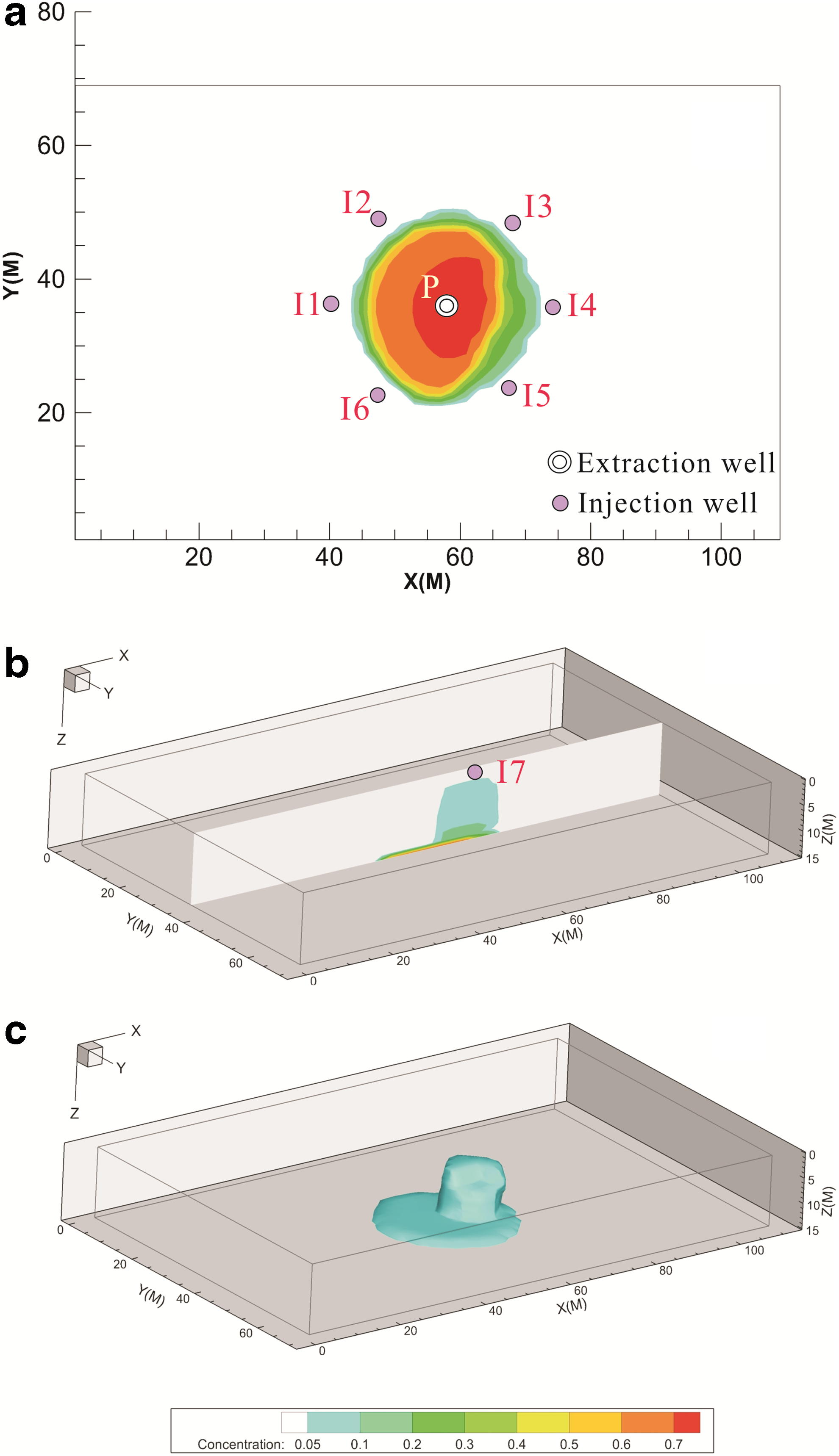
The practical application of the surrogate models and parameter optimization algorithms mentioned above was analyzed by using a hypothetical nitrobenzene-contaminated site as a case study. The site was located in the saturated zone of a 15 m depth aquifer with a complex mixture of clay and sand deposits, and the groundwater flowed in a right–left direction. The initial concentration (volume fraction) distribution at the site is shown in Fig. 3. Based on the contaminant distribution, a SEAR system, using sodium dodecyl benzene sulfonate as the surfactant, was designed with seven partially penetrating injection wells and one completely penetrating extraction well for the clean-up. Six injection wells were located around the contamination plume and the seventh was at the top. The extraction well was located in the central zone of the plume (Fig. 3). To maintain the groundwater balance, the extraction rate was set equal to the total injection rate. Surfactant flush was followed by water flush with the aim of clearing the residual surfactant and nitrobenzene as far as possible.
Initial distribution of nitrobenzene initial concentration distribution and locations of the extraction and injection wells. (a) Concentration distribution at X–Y plane (at layer 15); (b) concentration distribution slice at X–Z plane (at column 35); (c) 0.06 iso-surface of concentration distribution.
Multiphase flow numerical simulation model
A three-dimensional multiphase flow numerical model was developed to simulate the SEAR process. The model had the following characteristics: The aquifer is partially homogeneous with several interlayers and isotropic. The porosity had a constant value of 0.3 and the distribution of permeability is shown in Fig. 4. A first-type boundary condition was assigned to the left and right boundaries of the site, whereas the other boundaries were no-flux boundaries. The groundwater flowed in a right–left direction and the horizontal hydraulic gradient was set to 0.0112. The simulation domain was discretized into 15 vertical layers and each layer was further discretized into 55 × 35 grids, with each grid measuring 2 × 2 × 1 m3. The physical and chemical parameters of the site are listed in Table 1.
Permeability distribution. (a) Two-dimensional permeability distribution at X–Y plane (at layer 15); (b) Three-dimensional permeability distribution.
Physical and Chemical Parameters of Hypothetical Nitrobenzene-Contaminated Site
Parameter
Value
Longitudinal dispersivity
1 m
Transverse dispersivity
0.3 m
Water density
1,000 kg/m3
Nitrobenzene density
1,205 kg/m3
Surfactant density
1,090 kg/m3
Water viscosity
0.001 Pa·s
Nitrobenzene viscosity
0.00089 Pa·s
Nitrobenzene/water interfacial tension
0.02566 N/m
Nitrobenzene solubility in water
1,900 mg/L
Residual water saturation
0.24
Residual nitrobenzene saturation
0.17
The basis mass conservation equation for each component can be written as (Delshad et al., 1996):
\documentclass{aastex}\usepackage{amsbsy}\usepackage{amsfonts}\usepackage{amssymb}\usepackage{bm}\usepackage{yhmath, upgreek}\usepackage{mathrsfs}\usepackage{pifont}\usepackage{stmaryrd}\usepackage{textcomp}\usepackage{portland, xspace}\usepackage{amsmath, amsxtra}\pagestyle{empty}\DeclareMathSizes{10}{9}{7}{6}\begin{document}
\begin{align*}
{{{\partial} \left({ \phi {{ \tilde { C}}_k}{ \rho _k}} \right) }
\over {\partial t}} + \vec\nabla \left[ { \mathop\sum\limits_{l =
1}^{3} {\rho _k} \left( {{C_{kl}}{{ \vec v}_l} - \phi {S_l}{{\vec{
\vec{K}}}}_{kl}} \vec \nabla {C_{kl}} \right) } \right] = {R_k}
\tag{21}
\end{align*}
\end{document}
where k is component index, l is phase index, including water, oil, and surfactant (microemulsion), ø is porosity; \documentclass{aastex}\usepackage{amsbsy}\usepackage{amsfonts}\usepackage{amssymb}\usepackage{bm}\usepackage{yhmath, upgreek}\usepackage{mathrsfs}\usepackage{pifont}\usepackage{stmaryrd}\usepackage{textcomp}\usepackage{portland, xspace}\usepackage{amsmath, amsxtra}\pagestyle{empty}\DeclareMathSizes{10}{9}{7}{6}\begin{document}
$${ \tilde C_k}$$
\end{document} is overall concentration by volume fraction of component k; ρk is density of component k (kg/m3); Ckl is concentration by volume fraction of component k in phase l; \documentclass{aastex}\usepackage{amsbsy}\usepackage{amsfonts}\usepackage{amssymb}\usepackage{bm}\usepackage{yhmath, upgreek}\usepackage{mathrsfs}\usepackage{pifont}\usepackage{stmaryrd}\usepackage{textcomp}\usepackage{portland, xspace}\usepackage{amsmath, amsxtra}\pagestyle{empty}\DeclareMathSizes{10}{9}{7}{6}\begin{document}
$${ \vec v_l}$$
\end{document} is Darcy velocity of phase l (m/s); Sl is saturation of phase l; \documentclass{aastex}\usepackage{amsbsy}\usepackage{amsfonts}\usepackage{amssymb}\usepackage{bm}\usepackage{yhmath, upgreek}\usepackage{mathrsfs}\usepackage{pifont}\usepackage{stmaryrd}\usepackage{textcomp}\usepackage{portland, xspace}\usepackage{amsmath, amsxtra}\pagestyle{empty}\DeclareMathSizes{10}{9}{7}{6}\begin{document}
$$\vec{\vec{K}}$$
\end{document} is dispersion tensor (m2/s); Rk is total sources and sinks of component k (kg/[m3·s]).
The mathematical model was established by integrating the mass conservation equation and corresponding initial conditions and boundary conditions. UTCHEM (University of Texas Chemical Compositional Simulator), a popular software for simulating three-dimensional, multicomponent, multiphase, surfactant flooding processes, is used to solve the mathematical model.
Surrogate model of multiphase flow numerical simulation model
Luo and Lu (2014) researched the Sobol' sensitivity analysis of multiphase flow numerical simulation model. The results demonstrated that the remediation duration was the most important variable influencing remediation efficiency, followed by injection rates at wells, whereas the surfactant concentration had a negligible influence. Thus, with the aim of identifying the optimal SEAR strategy, remediation duration and injection/extraction rates at wells were treated as controllable input variables to build the surrogate model, whereas the surfactant concentration was set at a constant 4% (volume fraction). To reduce the dimension of input variables and improve the approximation accuracy, the injection rate at one well was set equal to the one at the diagonal site. The extraction rate was equal to the sum of injection rates. The water flush duration was set as 25 days with the same extraction/injection rates. Finally, the input vectors consisted of five elements: injection rates at I1, I2, I3, I7, and surfactant flush duration. The output variable was the nitrobenzene removal rate.
LHS method was used to obtain 100 training samples and 100 testing samples in feasible regions of the injection rates and remediation duration, which were taken as (10 and 60 m3/day) and (10 and 60 days), respectively. The 200 sets of remediation strategies were used as inputs for the developed simulation model and the corresponding outputs were obtained for the model runs.
RBFANN model was trained on the MATLAB platform by invoking the function of:
\documentclass{aastex}\usepackage{amsbsy}\usepackage{amsfonts}\usepackage{amssymb}\usepackage{bm}\usepackage{yhmath, upgreek}\usepackage{mathrsfs}\usepackage{pifont}\usepackage{stmaryrd}\usepackage{textcomp}\usepackage{portland, xspace}\usepackage{amsmath, amsxtra}\pagestyle{empty}\DeclareMathSizes{10}{9}{7}{6}\begin{document}
\begin{align*}
\rm{net} = \rm{newrb} \left( \rm{P , T , goal , spread , mn , df} \right) \tag{22}
\end{align*}
\end{document}
where P is the matrix of input vectors, T is the matrix of output vectors, goal is mean square error, spread is distribution density of RBF, mn is the maximum number of neurons, and df is the added number between two shows.
Following the training of the model, the testing and prediction were realized by invoking the function:
\documentclass{aastex}\usepackage{amsbsy}\usepackage{amsfonts}\usepackage{amssymb}\usepackage{bm}\usepackage{yhmath, upgreek}\usepackage{mathrsfs}\usepackage{pifont}\usepackage{stmaryrd}\usepackage{textcomp}\usepackage{portland, xspace}\usepackage{amsmath, amsxtra}\pagestyle{empty}\DeclareMathSizes{10}{9}{7}{6}\begin{document}
\begin{align*}{ \rm{y = sim}} \left( {{ \rm{net , X _- test}}} \right) \tag{23}\end{align*}
\end{document}
where X_test is the matrix of testing input vectors.
RBFANN, radial basis function artificial neural network.
Kriging model was built on the MATLAB platform by writing a program based on the above theory. The uncertain parameters \documentclass{aastex}\usepackage{amsbsy}\usepackage{amsfonts}\usepackage{amssymb}\usepackage{bm}\usepackage{yhmath, upgreek}\usepackage{mathrsfs}\usepackage{pifont}\usepackage{stmaryrd}\usepackage{textcomp}\usepackage{portland, xspace}\usepackage{amsmath, amsxtra}\pagestyle{empty}\DeclareMathSizes{10}{9}{7}{6}\begin{document}
$${ \alpha _i}$$
\end{document} were set as Table 3 shows.
Parameters of Kriging Model
α1
α2
α3
α4
α5
0.000917
0.000166
0.000176
0.000309
0.007644
Libsvm toolbox (Chang and Lin, 2001) was used to realize the training and testing of SVR model. The forms of invoked functions were as follows:
\documentclass{aastex}\usepackage{amsbsy}\usepackage{amsfonts}\usepackage{amssymb}\usepackage{bm}\usepackage{yhmath, upgreek}\usepackage{mathrsfs}\usepackage{pifont}\usepackage{stmaryrd}\usepackage{textcomp}\usepackage{portland, xspace}\usepackage{amsmath, amsxtra}\pagestyle{empty}\DeclareMathSizes{10}{9}{7}{6}\begin{document}
\begin{align*}
\begin{split}
&{\rm model} \\
& = {\rm svmtrain} (\text{P , T ,}^{\prime}\, \rm{-s} \;{\rm value} \ \rm{-t} \;{\rm value} \
\rm{-c} \;{\rm value} \ \rm{-g} \;{\rm value} \; \rm{-p} \; {\rm value}^{\prime}) \\
& \left[\text{Y ,} \;{\rm mse} \right] {\rm = svmpredict} \left(\text{Y\_-test , X \_- test , model}
\right)
\end{split}\tag{24}
\end{align*}
\end{document}
where s is the type of SVM model with the value 3 representing the SVR model; t is the type of kernel function with the value 2 representing the Gaussian function; and g is the parameter of Gaussian function, c and p are C and ɛ in Equation (10). The related parameters are shown in Table 4.
Parameters of SVR Model
S
t
c
G
p
3
2
9.986
0.453
0.00367
SVR, support vector regression.
The approximation effects of these models were objectively compared by optimizing their parameters using self-adaptive PSO.
Parameter optimization of surrogate model
To identify the parameter optimization algorithm for surrogate model among the algorithms mentioned above, Kriging model was selected as optimized object. The optimization model was established using the minimal sum of absolute error (absolute value) by fivefold cross-validation of the Kriging model with 100 training samples as the objective function, with the uncertain parameters \documentclass{aastex}\usepackage{amsbsy}\usepackage{amsfonts}\usepackage{amssymb}\usepackage{bm}\usepackage{yhmath, upgreek}\usepackage{mathrsfs}\usepackage{pifont}\usepackage{stmaryrd}\usepackage{textcomp}\usepackage{portland, xspace}\usepackage{amsmath, amsxtra}\pagestyle{empty}\DeclareMathSizes{10}{9}{7}{6}\begin{document}
$${ \alpha _i}$$
\end{document} in Equation (4) as decision variables. The constraints were the range of \documentclass{aastex}\usepackage{amsbsy}\usepackage{amsfonts}\usepackage{amssymb}\usepackage{bm}\usepackage{yhmath, upgreek}\usepackage{mathrsfs}\usepackage{pifont}\usepackage{stmaryrd}\usepackage{textcomp}\usepackage{portland, xspace}\usepackage{amsmath, amsxtra}\pagestyle{empty}\DeclareMathSizes{10}{9}{7}{6}\begin{document}
$${ \alpha _i}$$
\end{document}, which were empirically taken as (0, 10).
Use GA, self-adaptive PSO, and self-adaptive PSO based on SA to solve the optimization model by writing programs based on corresponding procedures on the MATLAB platform. The parameters of the optimization algorithms were set as Tables 5 and 6 show. When self-adaptive PSO based on SA was used for optimization, the annealing constant λ was set as 0.9; otherwise, the parameters were the same as those listed in Table 6 for self-adaptive PSO.
Parameters of GA
Parameter
Value
Population size
40
Maximum generations
300
Dimensionality of the problem
5
Generation gap
0.8
Crossover probability
0.7
Mutation probability
0.05
GA, genetic algorithm.
Parameters of Self-Adaptive PSO
Parameter
Value
Particle number
40
Maximum iterations
300
Dimensionality of the problem
5
wmax
0.9
wmin
0.4
c1
2
c2
2
PSO, particle swarm optimization.
The solving processes of three algorithms are similar. For GA, first initialize the population, which consists of a certain number of individuals in the form of binary code. Each individual is a sample of uncertain parameters \documentclass{aastex}\usepackage{amsbsy}\usepackage{amsfonts}\usepackage{amssymb}\usepackage{bm}\usepackage{yhmath, upgreek}\usepackage{mathrsfs}\usepackage{pifont}\usepackage{stmaryrd}\usepackage{textcomp}\usepackage{portland, xspace}\usepackage{amsmath, amsxtra}\pagestyle{empty}\DeclareMathSizes{10}{9}{7}{6}\begin{document}
$${ \alpha _i}$$
\end{document}. Then, the individuals are translated into decimal form so that they can be evaluated by computing their objective function values. Proceed selection, crossover, and mutation in the form of binary code according to the evaluation results. After the new generation is generated, repeat the previous works and go through this troop cycle until the final generation. The optimal solution can be obtained by decoding the optimal individual in the final generation.
For self-adaptive PSO and self-adaptive PSO based on SA, the initial positions of particles are the samples of uncertain parameters \documentclass{aastex}\usepackage{amsbsy}\usepackage{amsfonts}\usepackage{amssymb}\usepackage{bm}\usepackage{yhmath, upgreek}\usepackage{mathrsfs}\usepackage{pifont}\usepackage{stmaryrd}\usepackage{textcomp}\usepackage{portland, xspace}\usepackage{amsmath, amsxtra}\pagestyle{empty}\DeclareMathSizes{10}{9}{7}{6}\begin{document}
$${ \alpha _i}$$
\end{document}, and the speeds of particles are related to their positions. Evaluate particles by objective function values, then compute the inertia weight, and update the speeds and positions of particles according to Equations (12) and (13). Repeat the previous works in a loop to the maximum number of iterations, and make the gbest optimal solution.
Results and Discussions
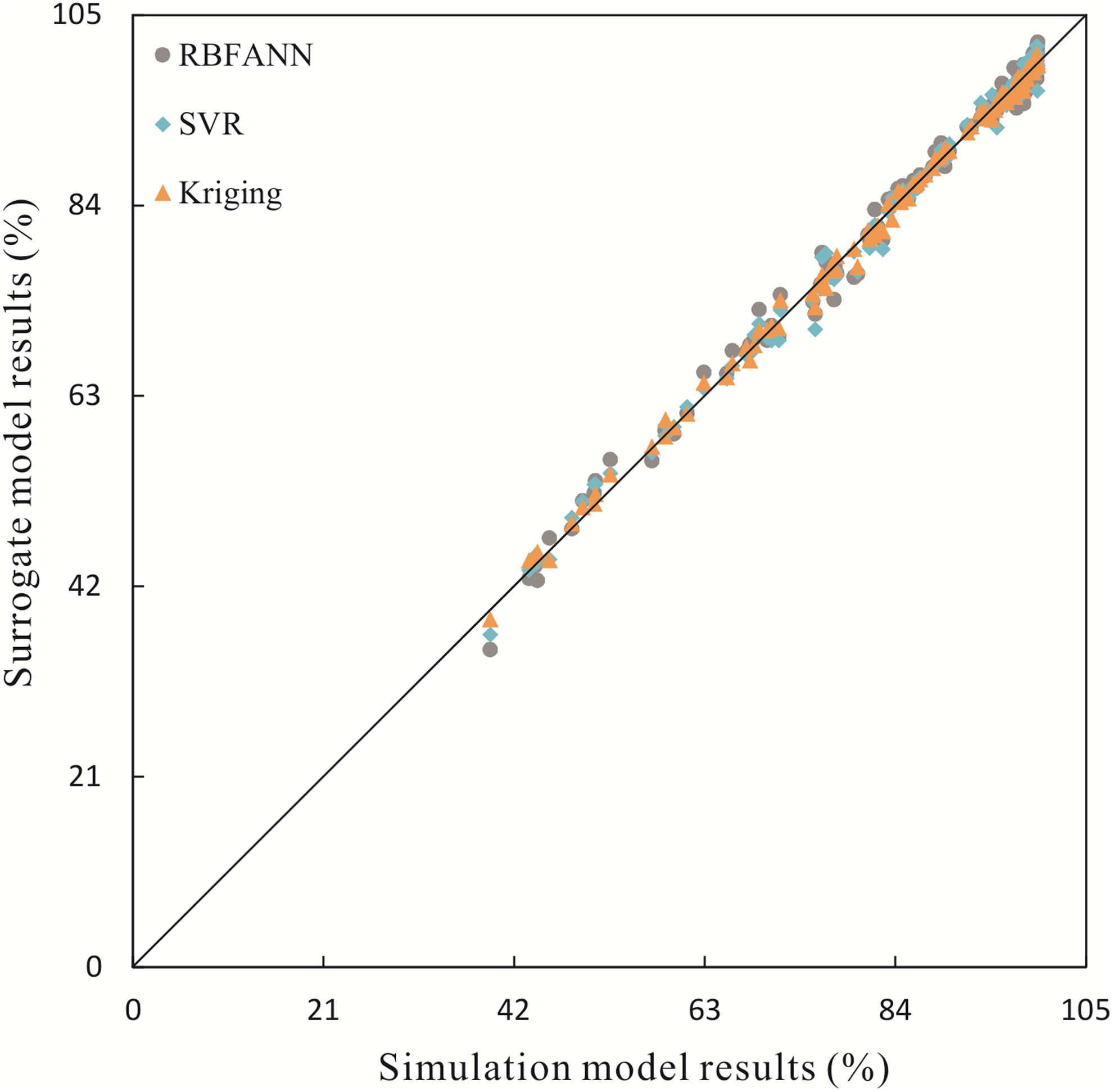
The removal rates of the 100 testing samples obtained using the trained RBFANN, SVR, and Kriging models were compared with those obtained using the developed simulation model and the results are presented in Fig. 5. The comparison demonstrated that the scatter related to Kriging model was the closest to the 1:1 perfect line for the validation phase, thereby indicating the highest approximation accuracy. This was followed by SVR model, with the RBFANN model being the least accurate. Relative errors (absolute value) of the removal rates between the surrogate models and simulation model using 100 testing samples are plotted in Fig. 6. The error level of Kriging model was obviously lower than the others. The performance of three surrogate models can also be evaluated and compared according to the five indices in Table 7. Kriging model is outstanding for all the indices.
Surrogate model results versus simulation results.
Distributions of relative errors for different surrogate models. (a) Distribution of relative errors in different intervals; (b) relative error cumulative frequency curve.
Performance Evaluation of Three Different Surrogate Models
Performance evaluation indices
Certainty coefficient R2
Mean absolute error (%)
Max absolute error (absolute value) (%)
Mean relative error (%)
Max relative error (absolute value) (%)
RBFANN
0.9917
1.1536
4.3227
1.5468
8.6584
SVR
0.9940
0.9231
4.4123
1.2748
6.4440
Kriging
0.9975
0.6116
2.7063
0.8501
3.3873
To improve the approximation accuracy, an attempt was made to reduce the dimension of input variables. But for the high-dimensional problem that dimension cannot be reduced, the advantages of SVR method will highlight. Whether the approximation accuracy of SVR model is really superior to that of Kriging model for high-dimensional problems would require further research to verify.
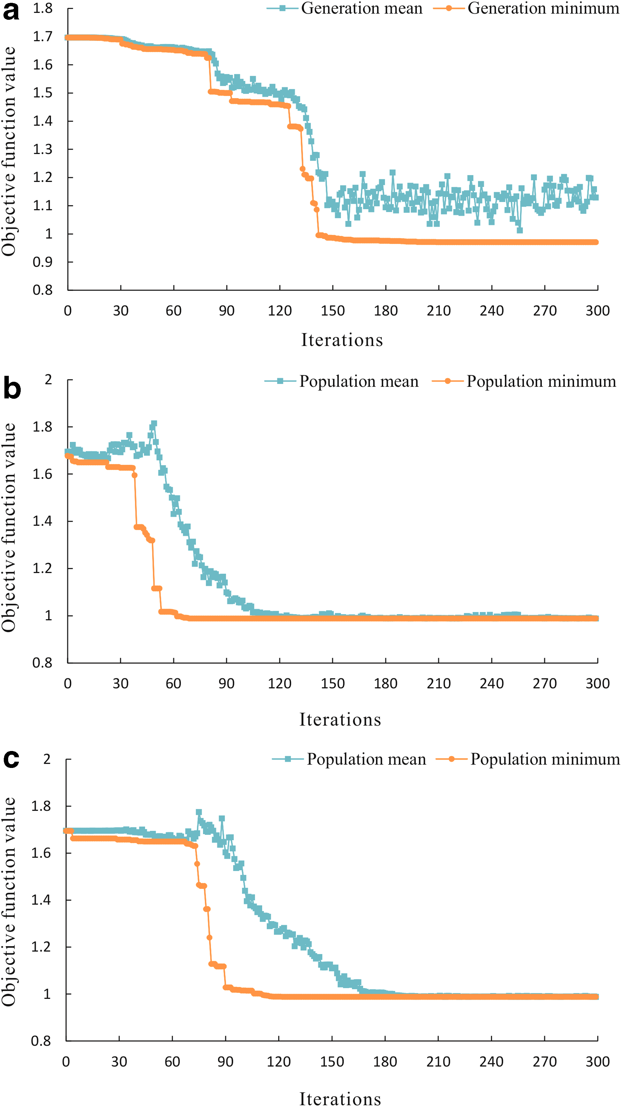
The computational efficiency of the algorithms varied, whereas GA required a considerable amount of time to search for the global optimal parameters, self-adaptive PSO was more efficient and improved the convergence speed (Fig. 7). However, these two algorithms may both be trapped in local minimal solutions (Fig. 8). In contrast, self-adaptive PSO based on SA, which incorporates the advantages of both PSO and SA, rapidly searched for the global optimum, and avoided entrapment in a local minimal solution. Once the parameter was optimized, the performance of Kriging model was significantly improved (Table 8), and its certainty coefficient (R2) reached 0.9975.
Convergence of objective function value during optimization process. (a) Genetic algorithm (GA); (b) self-adaptive particle swarm optimization (PSO); (c) self-adaptive PSO based on simulated annealing.
Cases of trapping entrapment in local minimal solutions. (a) GA; (b) self-adaptive PSO.
Performance Evaluation of Kriging Models With and Without Optimization
Performance evaluation indices
Certainty coefficient R2
Mean absolute error (%)
Max absolute error (absolute value) (%)
Mean relative error (%)
Max relative error (absolute value) (%)
With optimization
0.9918
1.1711
3.9907
1.5315
5.4863
Without optimization
0.9975
0.6116
2.7063
0.8501
3.3873
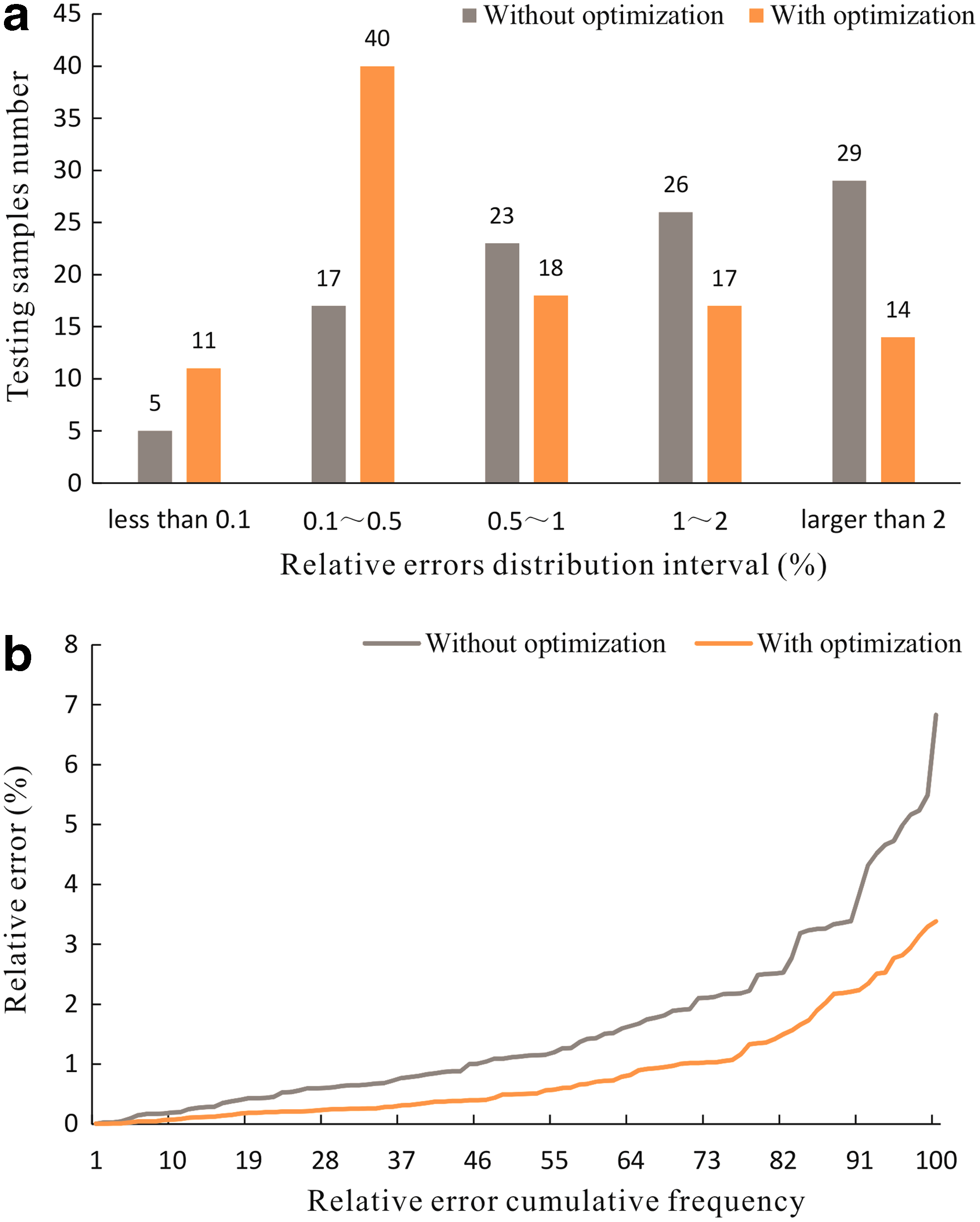
In conclusion, the optimal surrogate model is Kriging model for which the parameters were obtained by self-adaptive PSO based on SA. The relative errors (absolute value) of the removal rates between this surrogate model and the simulation model were below 3.5% using 100 testing samples. The MRE for the nitrobenzene removal rates was only 0.83%. The distribution of relative errors is presented in Fig. 9, where it can be seen that the relative errors mostly do not exceed 1%.
Distributions of relative errors for surrogate models with and without optimization. (a) Distribution of relative errors in different intervals; (b) relative error cumulative frequency curve.
Through selecting the optimal surrogate modeling method and parameter optimization algorithm, the approximation accuracy between surrogate model and simulation model or rather the reliability of surrogate model is remarkably increased. This result indicates that the surrogate model developed using Kriging method is capable of replacing the multiphase flow simulation model and that the applicability of surrogate-based simulation optimization technique is guaranteed. The efforts contribute to efficiently obtain a cost-effective and reliable SEAR strategy for DNAPL-contaminated site in practical application.
The iterative simulation optimization process of the numerical simulation model is computationally hugely expensive. The simulation of SEAR for the nitrobenzene-contaminated site required nearly 600 s of CPU time on a 3.0 GHz Intel core i3 CPU and 4 GB RAM PC platform. A conventional simulation optimization model required 20,000 iterations, which would require 12,000,000 s (139 days) of CPU time to process the overall simulation. However, each run of the surrogate model only requires 0.15 s. In comparison, building a surrogate model requires 100 training samples and 100 testing samples only, that is, 200 runs of the simulation model. Thus, replacing the simulation model with the Kriging surrogate model in the optimization process reduced the overall CPU time to 123,000 s (34 h).
In addition, surrogate model can be applied to many other problems, such as the hydrogeology parameters estimation based on a simulation model, multiphase flow transport sensitivity and uncertainty analysis, and contamination source inversion. Solving these problems requires thousands or even more simulation model computations. A surrogate can replace the input/output relationship of simulation model with far less computation time. It is the key for increasing the feasibility of solving related problems.
Conclusions
Replacing the simulation model with a surrogate model is an efficient way to reduce the huge computational burden produced by coupling simulation and optimization models. However, the reliability of such a simulation optimization model for groundwater remediation is closely related to the approximation accuracy of surrogate model. In this study, a numerical simulation model for a hypothetical DNAPL-contaminated site was developed to identify the optimal surrogate modeling method and parameter optimization algorithm. The input/output dataset was generated using the LHS method. RBFANN, Kriging, and SVR methods were used to build surrogate models for the developed simulation model. GA, self-adaptive weighted PSO and self-adaptive weighted PSO based on SA were used to optimize the parameters of Kriging model.
The results showed that Kriging model with the parameters obtained by self-adaptive weighted PSO based on SA was the most reliable and could reasonably predict the system response under the given operating conditions. As an extension of the previous surrogate model research, the proposed surrogate model was selected by sufficient comparison. It is of tremendous assistance for efficiently obtaining a cost-effective and reliable SEAR strategy for DNAPL-contaminated site.
Although the MRE for the optimal surrogate model is acceptably low, there are still several samples with very large relative errors. The existence of such points increases the risk of failure of strategy obtained by the simulation surrogate optimization model. Future research would have to be devoted to solving this problem.
Footnotes
Acknowledgments
This study was supported by the National Nature Science Foundation of China (No. 41372237), National Major Science and Technology Program of China for Water Pollution Control and Treatment (No. 2012ZX07201-001), and Graduate Innovation Fund of Jilin University (No. 2015083).
Author Disclosure Statement
No competing financial interests exist.
References
1.
BennerM.L., MohtarR.H., and LeeL.S. (2002). Factors affecting air sparging remediation systems using field data and numerical simulations. J. Hazard.Mater., 95, 305.
2.
BoydJ.P. (2010). Six strategies for defeating the Runge Phenomenon in Gaussian radial basis functions on a finite interval [J]. Comput. Math. Appl., 60, 3108.
3.
ChangC.-C., and LinC.-J. (2001). LIBSVM: A Library for Support Vector Machines. Software Available at: www.csie.ntu.edu.tw/∼cjlin/libsvm (accessed May15, 2013).
4.
ChiuC.Y., LinY., et al. (2012). Parameter optimization for microlens arrays fabrication using genetic algorithms. J. Chin. Soc. Mech. Eng., 33, 525.
5.
DelshadM., PopeG.A., and SepehrnooriK. (1996). A compositional simulator for modeling surfactant enhanced aquifer remediation, 1. Formulation. J. Contam. Hydrol., 23, 303.
6.
Fernandez-GarciaD., BolsterD., Sanchez-VilaX., et al. (2012). A Bayesian approach to integrate temporal data into probabilistic risk analysis of monitored NAPL remediation. Adv. Water Resour., 36, 108.
7.
HeL., HuangG.H., ZengG.M., et al. (2008). An integrated simulation, inference, and optimization method for identifying groundwater remediation strategies at petroleum-contaminated aquifers in western Canada. Water Res. 42, 2629.
8.
HuJ.N., HuJ.J., LinH.B., et al. (2014). State-of-charge estimation for battery management system using optimized support vector machine for regression [J]. J. Power Sources, 269, 682.
9.
KeglB., KrzyakA., and NiemannH. (2000). Radial basis function networks and complexity regularization in function learning and classification. In: SanfeliuA. and VillanuevaJ.J., Eds., Proceedings of the 15th International Conference on Pattern Recognition, Barcelona, Spain: Vol. 2. Los Alamitos: IEEE Computer Society, p. 2081.
10.
LiM.S., HuangX.Y., LiuH.S., et al. (2013). Prediction of gas solubility in polymers by back propagation artificial neural network based on self-adaptive particle swarm optimization algorithm and chaos theory [J]. Fluid Phase Equilibr. 356, 11.
11.
LiY.C., ZhouX.Q., LuM.M., et al. (2014). Parameters optimization for machining optical parts of difficult-to-cut materials by genetic algorithm. Mater. Manuf.Process., 29, 9.
12.
LiuL. (2005). Modeling for surfactant-enhanced groundwater remediation processes at DNAPLs-contaminated sites. J. Environ. Inform., 5, 42.
13.
LiuW.H., MedinaM.A.Jr., ThomannW., et al. (2000). Optimization of intermittent pumping schedules for aquifer remediation using a genetic algorithm. J. Am.Leather Chem. Assoc., 36, 1335.
14.
LuW.X., ChuH.B., et al. (2013). Optimization of denser nonaqueous phase liquids-contaminated groundwater remediation based on Kriging surrogate model. Water Pract. Technol., 8, 304.
15.
LuengoJ., GarcíaS., and HerreraF. (2010). A study on the use of imputation methods for experimentation with Radial Basis Function Network classifiers handling missing attribute values: The good synergy between RBFNs and EventCovering method [J]. Neural Netw. 23, 406.
16.
LuoJ.N., and LuW.X. (2014). Sobol' sensitivity analysis of NAPL-contaminated aquifer remediation process based on multiple surrogates [J]. Comput. Geosci., 67, 110.
17.
LuoJ.N., LuW.X., XinX., et al. (2013). Surrogate model application to the identification of an optimal surfactant-enhanced aquifer remediation strategy for DNAPL-contaminated sites [J]. J. Earth Sci., 24, 1023.
18.
ManoochehriM., and KolahanF. (2014). Integration of artificial neural network and simulated annealing algorithm to optimize deep drawing process [J]. Int. J. Adv. Manufact. Technol., 73, 241.
19.
MoradkhaniH., HsuK., GuptaH.V., et al. (2004). Improved streamflow forecasting using self-organizing radial basis function artificial neural networks. J. Hydrol., 295, 246.
20.
NavarroF.F., MartínezC.H., RamírezM.C., et al. (2011). Evolutionary q-Gaussian radial basis function neural network to determine the microbial growth/no growth interface of Staphylococcus aureus [J]. Appl. Soft Comput., 11, 3012.
21.
QinX.S., HuangG.H., ChakmaA., et al. (2007). Simulation-based process optimization for surfactant-enhanced aquifer remediation at heterogeneous DNAPL-contaminated sites. Sci. Total Environ., 381, 17.
22.
RahbehM.E., and MohtarR.H. (2006). Application of multiphase transport models to field remediation by air sparging and soil vapor extraction. J. Hazard. Mater., 143, 156.
23.
RegisR.G. (2011). Stochastic radial basis function algorithms for large-scale optimization involving expensive black-box objective and constraint functions [J]. Comput. Oper. Res., 38, 837.
24.
SacksJ., WelchW.J., MitchellT.J., et al. (1989). Design and analysis of computer experiments [J]. Stat. Sci., 4, 409.
25.
ShenW., GuoX., WuC., et al. (2010). Forecasting stock indices using radial basis function neural networks optimized by artificial fish swarm algorithm. Knowl. Based Syst., 3, 378.
26.
SmolaA.J., and ScholkopfB. (2004). A tutorial on support vector regression [J]. Stat. Comput., 14, 199.
27.
SreekanthJ., and DattaB. (2010). Multi-objective management of saltwater intrusion in coastal aquifers using genetic programming and modular neural network based surrogate models. J. Hydrol., 393, 245.
28.
SunJ., and LiJ. (2009). An improved self-adaptive particle swarm optimization algorithm with simulated annealing. In: LuoQ. and ZhuM., Eds., Third International Symposium on Intelligent Information Technology Application, Nanchang, China: Vol. 3. Los Alamitos: IEEE Computer Society, p. 396.
29.
WangF.K., and HuangP.R. (2014). Implementing particle swarm optimization algorithm to estimate the mixture of two Weibull parameters with censored data. J. Stat. Comput. Simulat., 84, 1975.
30.
ZhangY.S., KimbergD.Y., et al. (2014). Multivariate lesion-symptom mapping using support vector regression [J]. Hum. Brain Mapp., 35, 5861.