Bayesian Regularized Back-Propagation Neural Network Model for Chlorophyll-a Prediction: A Case Study in Meiliang Bay,Lake Taihu

Abstract

A Bayesian regularized back-propagation neural network (BRBPNN) model is created and used to predict the monthly chlorophyll-a concentration dynamics over a period of 15 years in Meiliang Bay, Lake Taihu. The optimal network was found to consist of seven input neurons, six hidden neurons, and one output neuron, and coefficient of determination (R²) values for the training, validation, and test sets were 0.77, 0.49, and 0.76, respectively. Respective values of the root mean square (RMSE) and bias for the three data sets are 17.24 and −1.05 for training, 12.48 and 0.62 for validation, and 11.01 and 2.2 for testing. Compared with multiple linear regression models, the BRBPNN model fit the data much better. Thus, the BRBPNN model was shown to be a powerful tool for predicting the long-term chlorophyll-a concentration dynamics in Meiliang Bay. Furthermore, we find that algae in the Meiliang Bay, principally Microcystis, were alkalophilic, and phytoplankton production was controlled by P inputs from spring to early summer, whereas N played a more dominant controlling role in summer–fall. Therefore, reducing P may no longer be adequate for Lake Taihu, and new nutrient reduction strategies should incorporate N-input reduction along with P-input reductions.

Introduction

Eutrophication is one of the most severe global ecological problems in freshwater and coastal marine ecosystems (Khan and Ansari, 2005). It not only degrades the waterbody but also causes the loss of ecological services provided by the aquatic ecosystems (Smith, 2003; Duan et al., 2009). Among all the consequences of the accelerated eutrophication of lakes and reservoirs, algal blooms are the most common visible symptom (Dokulil and Teubner, 2000).

Lake Taihu, the third largest freshwater lake in China, was oligotrophic in the 1950s, but the increase in anthropogenic nutrient input to the lake has resulted in algal blooms appearing since the 1990s (Chang, 1995). Meiliang Bay, situated at the northern end of Lake Taihu, is one of the most eutrophic bays in China and generally suffers more intense blooms than the open water of the lake (Chen et al., 2003; Liu et al., 2011). Lake Taihu not only plays an extremely important role in the economic and social development of the Yangtze River Delta but also provides irreplaceable ecological services to nearby regions. Thus, the issue of algal blooms in Lake Taihu has become prominent in China (Song et al., 2007; Wu et al., 2010).

To alleviate the harmful impact of algal blooms, it is imperative to determine the key factors governing the algal dynamics and to establish models that can effectively simulate the timing and magnitude of algal blooms (Wei et al., 2001). In recent years, artificial neural networks (ANNs) have been applied to predict algal blooms (Wu et al., 2013; Cho et al., 2014; Coad et al., 2014; Liu et al., 2015).

Based on the 1.5-year measured data set of Chla and environmental variables, Wu et al. (2013) developed ANN to simulate the daily Chla dynamics in a German lowland river, and the developed ANN models achieved satisfactory accuracy in predicting daily dynamics of Chla concentrations. Cho et al. (2014) used the automatic water quality monitoring data, weather data, and hydrologic data in the man-made Lake Juam during 2008–2010 to develop an ANN model to predict Chla concentration as an indirect measure of the abundance of algae, and the ANN trained with the time series data successfully predicted the Chla dynamics. Coad et al. (2014) used a high-resolution temporal data set, including Chla, temperature (water and air), salinity, and photosynthetically available radiation, to configure an ANN to predict (1, 3, and 7 days in advance) the Chla concentrations and obtained a satisfactory result.

These studies revealed that, compared with other modeling approaches, ANNs exhibit better performance in the prediction of algal blooms and have, therefore, become a popular and useful tool for environmental simulations (Maier and Dandy, 2001). Liu et al. (2015) used water quality and meteorological data from 1999 to 2012 in the Yuqiao Reservoir (Tianjin, China) to build six artificial networks (ANNs) to predict the levels of Chla and found that the back program model yielded slightly better results than all the other ANNs. Compared with other traditional ANNs, the Bayesian regularized back-propagation neural network (BRBPNN) performs better when the variables have a nonlinear relationship (Xu et al., 2006).

BRBPNNs have an excellent generalization capability, a result of their automated regularization parameter selection. This allows them to obtain the optimal network architecture for the posterior distribution and avoid the over-fitting problem (Mackay, 1992; Foresee and Hagan, 1997; Burden and Winkler, 2000).

In this study, a BRBPNN model is used to predict the chlorophyll-a concentrations in Meiliang Bay, Lake Taihu. The relative importance of environmental factors affecting the chlorophyll-a concentration is evaluated through a sensitivity analysis. We also compared the BRBPNN model with multiple linear regression (MLR) models. Finally, we provide some bases for the effective eutrophication treatment of Meiliang Bay.

Material and Methods

Study area and data

Lake Taihu has an area of 2,338 km² and an average depth of about 2.0 m. It is located between 30°05′ and 32°08′ N and 119°08′ and 121°55′ E, downstream of the Yangtze River (Fig. 1).

FIG. 1.

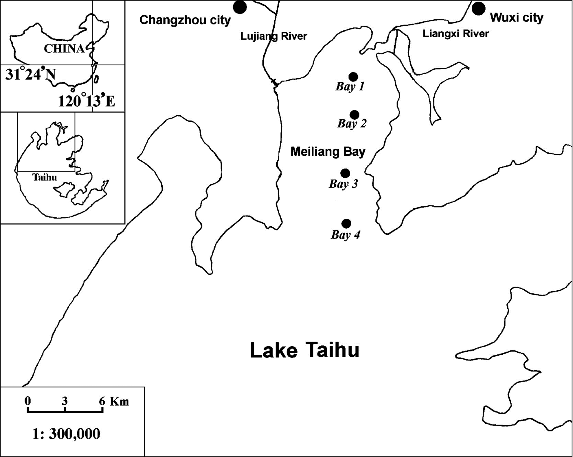
Location of Lake Taihu, China, and sampling sites in Meiliang Bay (northern Lake Taihu).

Meiliang Bay, situated in the northern part of Lake Taihu, is one of the most eutrophic bays (Chen et al., 2003). The bay has a surface area of 132 km² and a mean depth of 2.0 m. The Liangxi and the Lujiang rivers discharge wastewater from the cities of Wuxi and Changzhou into Meiliang Bay. Due to the heavy industrial and agricultural pollution, algal blooms have been frequently observed in Meiliang Bay during the past two decades (Liu et al., 2011; Paerl et al., 2011).

The water quality data used in this study were obtained from the Taihu Laboratory for Lake Ecosystem Research (CNERN TaiLLER). We selected monthly data over a period of 15 years (January 1992 to December 2006) and measured at four sites in the Meiliang Bay. The data include eight water quality factors such as pH, water temperature (WT, °C), transparency (SD, m), suspended solids (SS, mg/L), electrical conductivity (EC, μS/cm), total nitrogen (TN, mg/L), total phosphorus (TP, mg/L), and the chlorophyll-a concentration (Chla, μg/L). The basic statistics of the measured water quality variables in Meiliang Bay, Lake Taihu, is shown in Table 1. The raw data figure for eight water quality variables of four sampling points in Meiliang Bay is shown in Supplementary Fig. S1–S8.

Table 1.

Basic Statistics of the Measured Water Quality Variables in Meiliang Bay, Lake Taihu (n = 720)

Variable	Unit	Minimum	Maximum	Median	Mean	SD	CV (%)
pH	—	6.90	10.10	8.25	8.35	0.45	5.44
TN	mg/L	0.63	10.92	2.77	3.25	1.85	56.98
TP	mg/L	0.01	2.133	0.10	0.12	0.08	64.70
WT	°C	1.50	32.20	18.05	17.56	8.51	48.44
SD	m	0.10	1.50	0.40	0.47	0.21	45.38
SS	mg/L	1.60	192.60	34.48	39.64	25.25	63.70
EC	μS/cm	26.00	830.00	400.00	414.38	124.12	29.95
Chla	μg/L	0.00	521.73	16.28	25.58	30.75	120.21

CV, coefficient of variation; SD, standard deviation.

Bayesian regularized back-propagation neural network modeling

In general, a neural network comprises three layers: the input layer, the hidden layer(s), and the output layer. In this study, we build a three-layer neural network model, as shown in Fig. 2. Seven of the measured environmental factors are selected as the input layer variables. A single hidden layer is used, and the current month chlorophyll-a concentration, which is a well-known integrative indicator of algal biomass, is the output variable. All the computations were performed using MATLAB (MathWorks, Inc.).

FIG. 2.

Neural network structure.

Bayesian regularization algorithm

Many algorithms can be used to train neural network models. In this study, a Bayesian regularization algorithm is applied to the training data to calculate the weights between the input and hidden layers and between the hidden and output layers. The transfer functions of the hidden layer and output layer are set to the log–sigmoid function: \documentclass{aastex}\usepackage{amsbsy}\usepackage{amsfonts}\usepackage{amssymb}\usepackage{bm}\usepackage{mathrsfs}\usepackage{pifont}\usepackage{stmaryrd}\usepackage{textcomp}\usepackage{portland, xspace}\usepackage{amsmath, amsxtra}\pagestyle{empty}\DeclareMathSizes{10}{9}{7}{6}\begin{document} \begin{align*}f ( x ) = 1 / ( 1 - e^x ) , \tag{1}\end{align*} \end{document}

where x is the input vector.

The BRBPNN uses the regularization method to improve its generalization ability. The training objective function F is given by the following: \documentclass{aastex}\usepackage{amsbsy}\usepackage{amsfonts}\usepackage{amssymb}\usepackage{bm}\usepackage{mathrsfs}\usepackage{pifont}\usepackage{stmaryrd}\usepackage{textcomp}\usepackage{portland, xspace}\usepackage{amsmath, amsxtra}\pagestyle{empty}\DeclareMathSizes{10}{9}{7}{6}\begin{document} \begin{align*}F = \alpha E_W + \beta E_D , \tag{2}\end{align*} \end{document}

where E_w is the squared sum of the weights in the network, E_D is the squared sum of the residuals between network response values and objective values, and α, β are objective function parameters or hyperparameters.

In the Bayesian framework, the weights of the network are considered to be random variables. At first, the function is set to some prior distribution. When the data have been observed, the posterior distribution of the weights can be updated using Bayes' rule: \documentclass{aastex}\usepackage{amsbsy}\usepackage{amsfonts}\usepackage{amssymb}\usepackage{bm}\usepackage{mathrsfs}\usepackage{pifont}\usepackage{stmaryrd}\usepackage{textcomp}\usepackage{portland, xspace}\usepackage{amsmath, amsxtra}\pagestyle{empty}\DeclareMathSizes{10}{9}{7}{6}\begin{document} \begin{align*}P ( w \mid D , \alpha , \beta , G ) = \frac { P ( D \mid w , \beta , G ) P ( w \mid \alpha , G ) } { P ( D \mid \alpha , \beta , G ) } , \tag { 3 } \end{align*} \end{document}

where G is the neural network model, w is the vector of network weights, P(w|α,G) is the prior density, P(D|w,β,G) is the likelihood function, and P(D|α,β,G)is the normalization factor (Mackay, 1992). Thus, Equation (3) can be expressed as follows: \documentclass{aastex}\usepackage{amsbsy}\usepackage{amsfonts}\usepackage{amssymb}\usepackage{bm}\usepackage{mathrsfs}\usepackage{pifont}\usepackage{stmaryrd}\usepackage{textcomp}\usepackage{portland, xspace}\usepackage{amsmath, amsxtra}\pagestyle{empty}\DeclareMathSizes{10}{9}{7}{6}\begin{document} \begin{align*}Posterior = \frac { Likelihood \cdot Prior } { Evidence } . \tag { 4 } \end{align*} \end{document}

Assuming that the weight and data probability distributions are Gaussian, the likelihood function can be written as follows: \documentclass{aastex}\usepackage{amsbsy}\usepackage{amsfonts}\usepackage{amssymb}\usepackage{bm}\usepackage{mathrsfs}\usepackage{pifont}\usepackage{stmaryrd}\usepackage{textcomp}\usepackage{portland, xspace}\usepackage{amsmath, amsxtra}\pagestyle{empty}\DeclareMathSizes{10}{9}{7}{6}\begin{document} \begin{align*}P ( D \mid w , \beta , G ) = \frac { \exp ( - \beta E_D ) } { Z_W ( \beta ) } , \tag { 5 } \end{align*} \end{document}

where Z_D(β) is the normalization factor: \documentclass{aastex}\usepackage{amsbsy}\usepackage{amsfonts}\usepackage{amssymb}\usepackage{bm}\usepackage{mathrsfs}\usepackage{pifont}\usepackage{stmaryrd}\usepackage{textcomp}\usepackage{portland, xspace}\usepackage{amsmath, amsxtra}\pagestyle{empty}\DeclareMathSizes{10}{9}{7}{6}\begin{document} \begin{align*}Z_D ( \beta ) = ( \pi / \beta ) ^{n / 2}. \tag{6}\end{align*} \end{document}

Similarly, the prior probability can be written as follows: \documentclass{aastex}\usepackage{amsbsy}\usepackage{amsfonts}\usepackage{amssymb}\usepackage{bm}\usepackage{mathrsfs}\usepackage{pifont}\usepackage{stmaryrd}\usepackage{textcomp}\usepackage{portland, xspace}\usepackage{amsmath, amsxtra}\pagestyle{empty}\DeclareMathSizes{10}{9}{7}{6}\begin{document} \begin{align*}P ( w \mid \alpha , G ) = \frac { \exp ( - \alpha E_W ) } { Z_W ( \alpha ) } , \tag { 7 } \end{align*} \end{document}

where Z_W(α) is the normalization factor: \documentclass{aastex}\usepackage{amsbsy}\usepackage{amsfonts}\usepackage{amssymb}\usepackage{bm}\usepackage{mathrsfs}\usepackage{pifont}\usepackage{stmaryrd}\usepackage{textcomp}\usepackage{portland, xspace}\usepackage{amsmath, amsxtra}\pagestyle{empty}\DeclareMathSizes{10}{9}{7}{6}\begin{document} \begin{align*}Z_D ( \alpha ) = ( \pi / \alpha ) ^{k / 2}. \tag{8}\end{align*} \end{document}

Finally, the posterior probability can be written as follows: \documentclass{aastex}\usepackage{amsbsy}\usepackage{amsfonts}\usepackage{amssymb}\usepackage{bm}\usepackage{mathrsfs}\usepackage{pifont}\usepackage{stmaryrd}\usepackage{textcomp}\usepackage{portland, xspace}\usepackage{amsmath, amsxtra}\pagestyle{empty}\DeclareMathSizes{10}{9}{7}{6}\begin{document} \begin{align*}P ( w \mid D , \alpha , \beta , G ) = \frac { \exp ( - F ( w ) ) } { Z_F ( \alpha , \beta ) } . \tag { 9 } \end{align*} \end{document}

We use Bayes' rule to optimize the objective function parameters α and β. Thus, we have the following: \documentclass{aastex}\usepackage{amsbsy}\usepackage{amsfonts}\usepackage{amssymb}\usepackage{bm}\usepackage{mathrsfs}\usepackage{pifont}\usepackage{stmaryrd}\usepackage{textcomp}\usepackage{portland, xspace}\usepackage{amsmath, amsxtra}\pagestyle{empty}\DeclareMathSizes{10}{9}{7}{6}\begin{document} \begin{align*}P ( \alpha , \beta \mid D , G ) = \frac { P ( D \mid \alpha , \beta , G ) P ( \alpha , \beta \mid G ) } { P ( D \mid G ) } , \tag { 10 } \end{align*} \end{document}

where P(α,β|G) is the prior probability for the regularization parameters α and β, and P(D|α,β,G) is the likelihood function, which is called the evidence for α and β (Mackay, 1992). The optimum values for α and β can be inferred as Livingstone (2009): \documentclass{aastex}\usepackage{amsbsy}\usepackage{amsfonts}\usepackage{amssymb}\usepackage{bm}\usepackage{mathrsfs}\usepackage{pifont}\usepackage{stmaryrd}\usepackage{textcomp}\usepackage{portland, xspace}\usepackage{amsmath, amsxtra}\pagestyle{empty}\DeclareMathSizes{10}{9}{7}{6}\begin{document} \begin{align*}\alpha = \gamma / 2 E_W; \beta = ( n - \gamma ) / 2 E_D; \gamma = \sum_{i = 1}^m m - \alpha \cdot trace^{ - 1} ( A ) , \tag{11}\end{align*} \end{document}

where γ is the effective parameter, n is the number of sample sets, m is the total number of parameters in the network, and A is the Hessian matrix of the objective function F(w).

According to Foresee and Hagan (1997), the iterative procedure is as follows. (1) Initialize values for α, β, and the weights. (2) Employ one step of the Levenberg–Marquardt algorithm to minimize the objective function F(w). (3) Compute γ using the Gauss–Newton approximation to the Hessian matrix in the Levenberg–Marquardt training algorithm. (4) Compute new values for the objective function parameters α and β. (5) Iterate steps (2–4) until convergence.

BRBPNN training

The data were normalized for the input and output layers using the linear insert-value method, which is expressed as follows: \documentclass{aastex}\usepackage{amsbsy}\usepackage{amsfonts}\usepackage{amssymb}\usepackage{bm}\usepackage{mathrsfs}\usepackage{pifont}\usepackage{stmaryrd}\usepackage{textcomp}\usepackage{portland, xspace}\usepackage{amsmath, amsxtra}\pagestyle{empty}\DeclareMathSizes{10}{9}{7}{6}\begin{document} \begin{align*} \overline {\rm X} = 0.1 + 0.8 \frac {{{\rm X} - {\rm X} _ {\rm min}}} {{\rm X} _ {max} - {\rm X}_{min}} , \tag { 12 } \end{align*} \end{document}

where x is the original data and \documentclass{aastex}\usepackage{amsbsy}\usepackage{amsfonts}\usepackage{amssymb}\usepackage{bm}\usepackage{mathrsfs}\usepackage{pifont}\usepackage{stmaryrd}\usepackage{textcomp}\usepackage{portland, xspace}\usepackage{amsmath, amsxtra}\pagestyle{empty}\DeclareMathSizes{10}{9}{7}{6}\begin{document} $$\overline{x}$$ \end{document} is the normalized data; X_min and X_max are the minimum and maximum values of the original data.

The first 9 years of data (1992–2000) of all the four sampling points were used for model training, and data of 2001, 2003, and 2005 were used as the validation data set. The remaining 3 years (2002, 2004, and 2006) were used for model testing.

Modeling performance criteria

To determine the performance of the developed BRBPNN model, three different criteria were used: the root mean square (RMSE), the bias, and the coefficient of determination (R²) (Chenard and Caissie, 2008; Singh et al., 2009). The RMSE represents the error associated with the model and can be computed as follows: \documentclass{aastex}\usepackage{amsbsy}\usepackage{amsfonts}\usepackage{amssymb}\usepackage{bm}\usepackage{mathrsfs}\usepackage{pifont}\usepackage{stmaryrd}\usepackage{textcomp}\usepackage{portland, xspace}\usepackage{amsmath, amsxtra}\pagestyle{empty}\DeclareMathSizes{10}{9}{7}{6}\begin{document} \begin{align*} { \rm RMSE } = \sqrt { \mathop \sum \limits_ { { \rm i } = 1 } ^ { \rm N } \frac { ( { \rm P_i } - { \rm M_i } ) ^2 } { { \rm N } } } , \tag { 13 } \end{align*} \end{document}

where P_i and M_i represented the model computed and the measured values of the variables, and the N represents the number of observations.

The bias represents the mean of all the individual errors and indicates whether the model overestimates or underestimates the dependent variable. It is calculated as follows: \documentclass{aastex}\usepackage{amsbsy}\usepackage{amsfonts}\usepackage{amssymb}\usepackage{bm}\usepackage{mathrsfs}\usepackage{pifont}\usepackage{stmaryrd}\usepackage{textcomp}\usepackage{portland, xspace}\usepackage{amsmath, amsxtra}\pagestyle{empty}\DeclareMathSizes{10}{9}{7}{6}\begin{document} \begin{align*} { \rm Bias } = \sqrt { \mathop \sum \limits_ { { \rm i } = 1 } ^ { \rm N } \frac { ( { \rm P_i } - { \rm M_i } ) ^2 } { { \rm N } } } . \tag { 14 } \end{align*} \end{document}

The coefficient of determination (R²) represents the percentage of variability that can be explained by the model and is calculated as follows:

where parameters have been defined in Equation (15).

Results and Discussion

Determination of BRBPNN structure

Generally, the number of hidden layers in a traditional BPNN is determined by repeatedly testing the network. However, BRBPNN can automatically find the optimum value from the posterior distribution (Mackay, 1992; Foresee and Hagan, 1997).

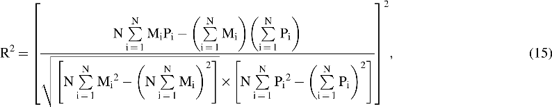
To acquire the optimal structure, the BRBPNNs were independently trained 20 times to eliminate spurious effects caused by the random set of initial weights and 3,000 epochs of maximal stopping (Xu et al., 2006). From Fig. 3, we can see the trend in the number of neurons S in the hidden layer for an optimal network with 15 parallel training runs and 1,500 epochs of maximal stopping. As S increases up to a value of 6, the number of effective parameters increases and the mean squared error (MSE) becomes smaller. When S is greater than 6, the MSE and number of effective parameters remain roughly constant. This gives the minimum number of hidden neurons required to properly represent the objective function. Therefore, we can determine the optimal number of neurons in the input, hidden, and output layers as 7-6-1, respectively, in our BRBPNN model.

FIG. 3.

Change in the optimal Bayesian regularized back-propagation neural network (BRBPNN) along with the number of hidden neurons. MSE, mean squared error.

Training, validation, and testing results

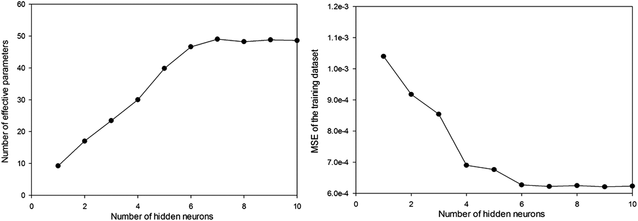
Table 2 shows the performance parameter of the BRBPNN model for computation of the monthly chlorophyll-a concentrations of different sampling points in Meiliang Bay, Lake Taihu. Figures 4 –6 show the training, validation, and testing results of (7-6-1) BRBPNN model for chlorophyll-a concentrations for four sampling points in the Meiliang Bay, Lake Taihu, respectively.

FIG. 4.

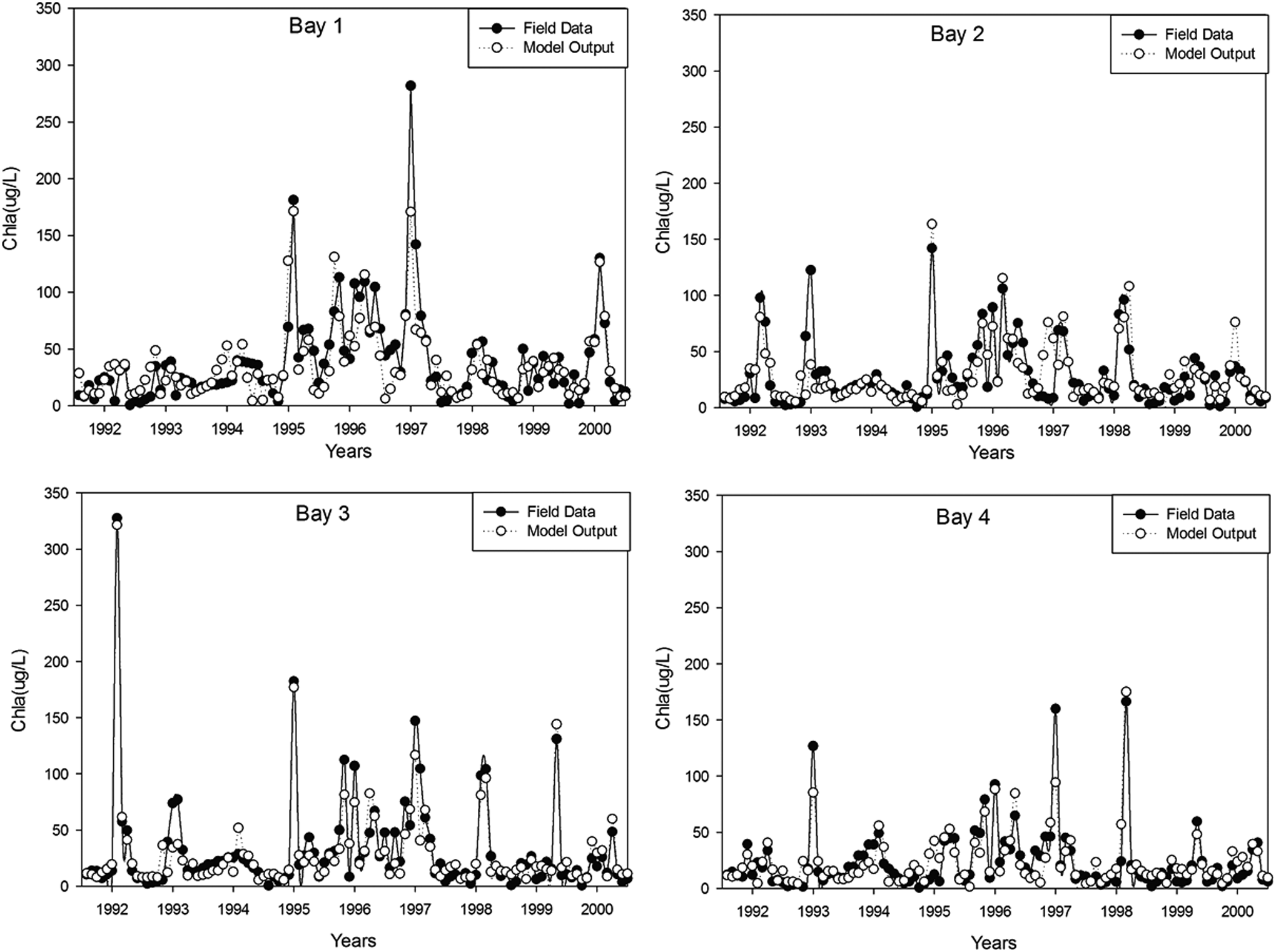
Training results of (7-6-1) BRBPNN model for chlorophyll-a concentrations for four sampling points from Meiliang Bay, Lake Taihu.

FIG. 5.

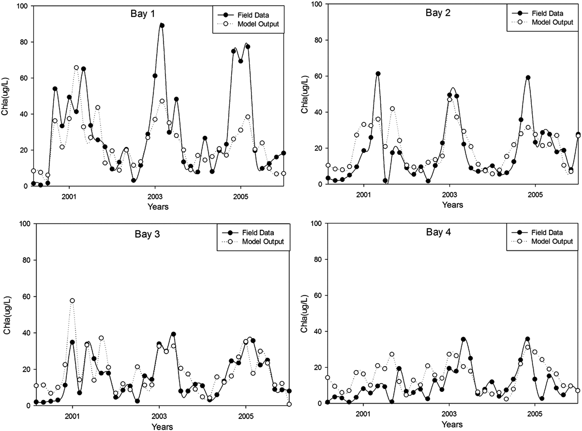
Validation results of (7-6-1) BRBPNN model for chlorophyll-a concentrations for four sampling points from in Meiliang Bay, Lake Taihu.

FIG. 6.

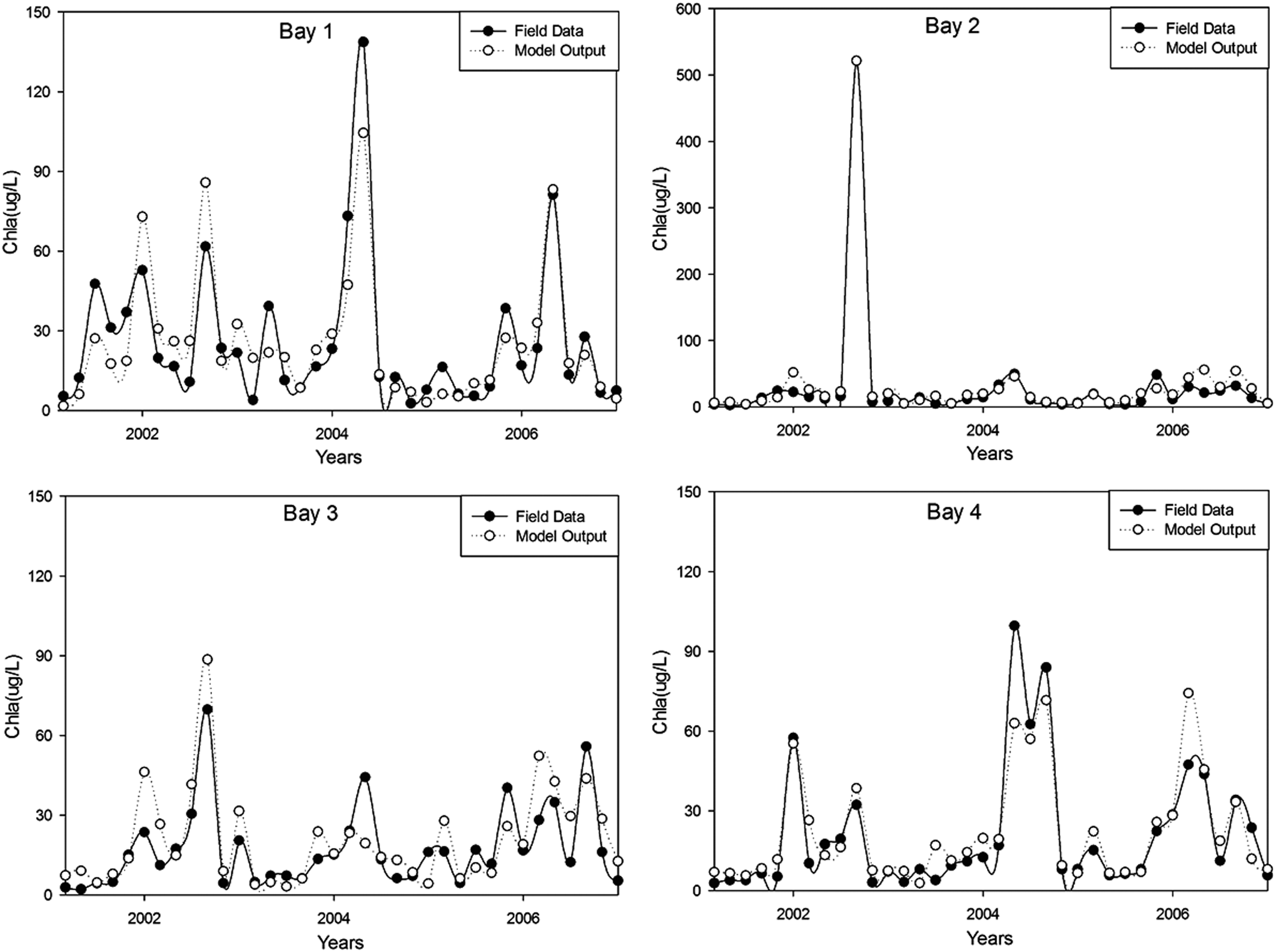
Testing results of (7-6-1) BRBPNN model for chlorophyll-a concentrations for four sampling points from in Meiliang Bay, Lake Taihu.

Table 2.

Performance Parameters of BRBPNN Model for Computation of the Monthly Chlorophyll-a Concentrations of Different Sampling Points in Meiliang Bay, Lake Taihu

Sampling point	RMSE	Bias	R²
All of the four sampling points
Training	17.24	−1.05	0.77
Validation	12.48	0.62	0.49
Test	11.01	2.2	0.94
Training + Validation + Test	15.28	−0.06	0.81
Bay 1
Training	21.42	−2.84	0.72
Validation	18.20	−6.25	0.5
Test	12.52	−0.58	0.79
Training + Validation + Test	19.31	−3.07	0.71
Bay 2
Training	18.75	0.35	0.58
Validation	10.75	2.15	0.55
Test	11.17	4.87	0.98
Training + Validation + Test	16.09	1.61	0.86
Bay 3
Training	14.18	−1.80	0.90
Validation	8.92	2.55	0.53
Test	10.66	3.27	0.67
Training + Validation + Test	12.62	0.08	0.86
Bay 4
Training	13.32	0.1	0.77
Validation	9.76	4.07	0.20
Test	9.49	1.22	0.85
Training + Validation + Test	11.98	1.12	0.76

BRBPNN, Bayesian regularized back-propagation neural network; RMSE, the root mean square.

The coefficient of determination (R²) values (p < 0.001) for the training, validation, and test sets were 0.77, 0.49, and 0.76, respectively. The respective values of RMSE and bias for the three data sets are 17.24 and −1.05 for training, 12.48 and 0.62 for validation, and 11.01 and 2.2 for testing. A closely followed pattern of variation by the measured and model-computed chlorophyll-a concentrations in Meiliang Bay, Lake Taihu (Figs. 4 –6), R², RMSE, and bias values suggest for a good fit of the BRBPNN model to the data set. The respective values of RMSE and bias and the coefficient of determination (R²) for the four sampling points are 19.31, −3.07, and 0.71 for Bay 1, 16.09, 1.61, and 0.86 for Bay 2, 12.62, 0.08, and 0.86 for Bay 3, and 11.98, 1.12, and 0.76 for Bay 4.

Compared with other two sampling points, Bay 2 and Bay 3 yield slightly better results. This may be because, compared with the two sampling points in the middle of the bay, Bay 1 is closer to the shoreside and Bay 4 is closer to the mouth of the bay, the concentrations of chlorophyll-a in Bay 1 and Bay 4 are more likely to be distracted.

Furthermore, all of the field data and model output were divided into the following four groups: spring (March–May), summer (June–August), fall (September–November), and winter (December–January).

Then, we calculated the respective values of RMSE, bias, and the coefficient of determination (R²) for the four seasons. Table 3 shows the performance parameters of the BRBPNN model for computation of the monthly chlorophyll-a concentrations of different seasons in Meiliang Bay, Lake Taihu. The respective values of RMSE, bias, and the coefficient of determination (R²) for the four seasons are 14.31, 0.80, and 0.53 for spring, 22.10, −1.63, and 0.79 for summer, 12.35, 0.68, and 0.90 for fall, and 9.41, −0.1, and 0.38 for winter. Although the values of RMSE and bias for summer are slightly higher, caused by the high concentrations of chlorophyll-a in summer, the values of the coefficient of determination (R²) for summer are quite high.

Table 3.

Performance Parameters of BRBPNN Model for Computation of Monthly Chlorophyll-a Concentrations of Different Seasons in Meiliang Bay, Lake Taihu

Season	RMSE	Bias	R²
Spring	14.31	0.80	0.53
Summer	22.10	−1.63	0.79
Fall	12.35	0.68	0.90
Winter	9.41	−0.1	0.38

Thus, we can conclude that our BRBPNN model can be seen as a reliable tool to predict algal blooms and simulate the chlorophyll-a dynamics in Meiliang Bay, Lake Taihu.

Compared with MLR models

In recent years, MLR-based models have repeatedly been applied to many fields for predictions (Bruder et al., 2014; In Ieong et al., 2014; Tugcu et al., 2014). Bruder et al. (2014) used the MLR-based models to predict the taste and compounds in algal bloom-affected inland water bodies and obtained quite good simulation results. By using the MLR-based models, In Ieong et al. (2014) correctly predicted the phytoplankton abundance in Macau Storage Reservoir. Tugcu et al. (2014) presented quantitative structure–toxicity relationship models on the toxicity of 91 organic compounds to Chlorella vulgaris using MLR techniques. Thus, based on our data, we developed MLR models to predict the chlorophyll-a concentrations in Meiliang Bay, Lake Taihu, and compared the MLR-based models with our BRBPNN model.

All the data from the four stations were log transformed, and regression tests were applied to determine the relationships between chlorophyll-a concentration and other water quality variables. The MLR models and the values of the coefficients are shown in Table 4. Compared with the MLR models, the BRBPNN model fits the data much better. This suggested that the BRBPNN model could capture the complex relationships between chlorophyll-a concentration and other water quality variables. Thus, compared with the MLR models, the proposed BRBPNN model is a better way to predict the chlorophyll-a concentration in Meiliang Bay, Lake Taihu.

Table 4.

Multiple Linear Regression Models and Coefficient of Determination ( R ²)

Models	R²
lgChla = 10.497lgpH − 8.485	0.290
lgChla = 1.227 − 0.94lgTN	0.003
lgChla = 1.826 + 0.64lgTP	0.124
lgChla = 0.255 + 0.791lgWT	0.216
lgChla = 0.97 − 0.576lgSD	0.06
lgChla = 0.684 + 0.332lgSS	0.05
lgChla = 1.517 − 0.128lgEC	0.001
lgChla = 7.884lgpH + 0.361lgTN + 0.43lgTP − 5.413 + 0.526lgWT − 0.463lgEC + 0.124lgSS	0.458

Sensitivity analyses of the input variables

To identify the sensitivity of chlorophyll-a concentration to minor changes in each input factor, we conducted simulations by increasing each input parameter by 10%. The calculated results are shown in Table 5. The sensitivity analyses indicated that a positive relationship existed between Chla and pH. It is known that Microcystis is the dominant species in Lake Taihu (Zhang et al., 2015). We can conclude that algae in the Meiliang Bay, principally Microcystis, were alkalophilic.

Table 5.

Change in Chlorophyll-a Concentration with a 10% Increase in Each Input Factor (Mean ± Standard Deviation)

Input factors	Chlorophyll-a concentration (%)
pH	238.65 ± 242.92
TN	0.53 ± 1.90
TP	0.68 ± 0.72
WT	1.15 ± 2.96
SD	−0.48 ± 1.87
SS	−0.10 ± 0.27
EC	−0.09 ± 0.21

Wei et al. (2001) used an ANN to predict algal blooms in Lake Kasumigaura, Japan, and found that a 10% increase in pH value would lead to the increases of 59.1%, 67.4%, 100.3%, and 158.9% in the densities of Microcystis, Oscillatoria, Phormidium, and Synedra, respectively. Based on an 11-year set of environmental monitoring data in Meiliang Bay, Liu et al. (2011) found that pH was significantly correlated with Microcystis in Lake Taihu, Meiliang Bay. By means of evolutionary computation, Zhang et al. (2015) successfully developed forecasting models that provide early warning on cyanobacteria outbreaks in Lake Taihu and found that a positive relationship existed between cyanobacteria and pH.

Increased pH may in fact increase the availability of P and cause the algal proliferation (Brewer and Goldman, 1976). However, the algal photosynthetic process removes CO₂ from the water and causes the increase of pH (Xu et al., 2010). Therefore, it is difficult to establish whether low CO₂/high pH is the cause of, or the result of, increased growth of Microcystis in Meiliang Bay (Liu et al., 2011). Further research is needed to be done in this point.

As shown in Table 3, increase in TN or TP value also would cause the increase in chlorophyll-a concentration. However, compared with pH, a 10% increase in TN or TP value causes relatively a small change in chlorophyll-a concentration in the presented model output. This is because, according to the range of the pH value, a 10% increase is relatively large but not for the TN or TP. In most earlier research work of nutrient limitation to phytoplankton, Meiliang Bay has long been assumed to be P-limited based on year-scale data, as supported by analyses of TN:TP (Vant et al., 1998). Recent studies, however, have found that phytoplankton production was controlled by P inputs from spring to early summer, whereas N played a more dominant controlling role in summer–fall (Xu et al., 2010; Paerl et al., 2011; Xu et al., 2013; Paerl et al., 2014, 2015; Ye et al., 2015).

Thus, we conducted the following three simulations: (1) increase of input TN value 0.5 mg/L (+N); (2) increase of input TP value 0.02 mg/L (+P); and (3) both of input TN and TP value (Paerl et al., 2015). Figures 7 and 8 show the change of chlorophyll-a concentrations from spring to early summer (March−June) and summer–fall (July−October), respectively, in three simulations: (1) +N, (2) +P, and (3) +NP. From spring to early summer (March−June), +P and +NP had a statistically significant positive influence on Chla concentrations, whereas +N and +NP were more stimulatory in summer to fall (Figs. 7 and 8). This is because, at the beginning of spring, total dissolved nitrogen concentrations were often very high relative to dissolved inorganic phosphorus concentrations, whereas during summer–fall, when dissolved inorganic nitrogen levels rapidly decreased, the algae tended to show more significant growth responses to +N simulation (Paerl et al., 2015).

FIG. 7.

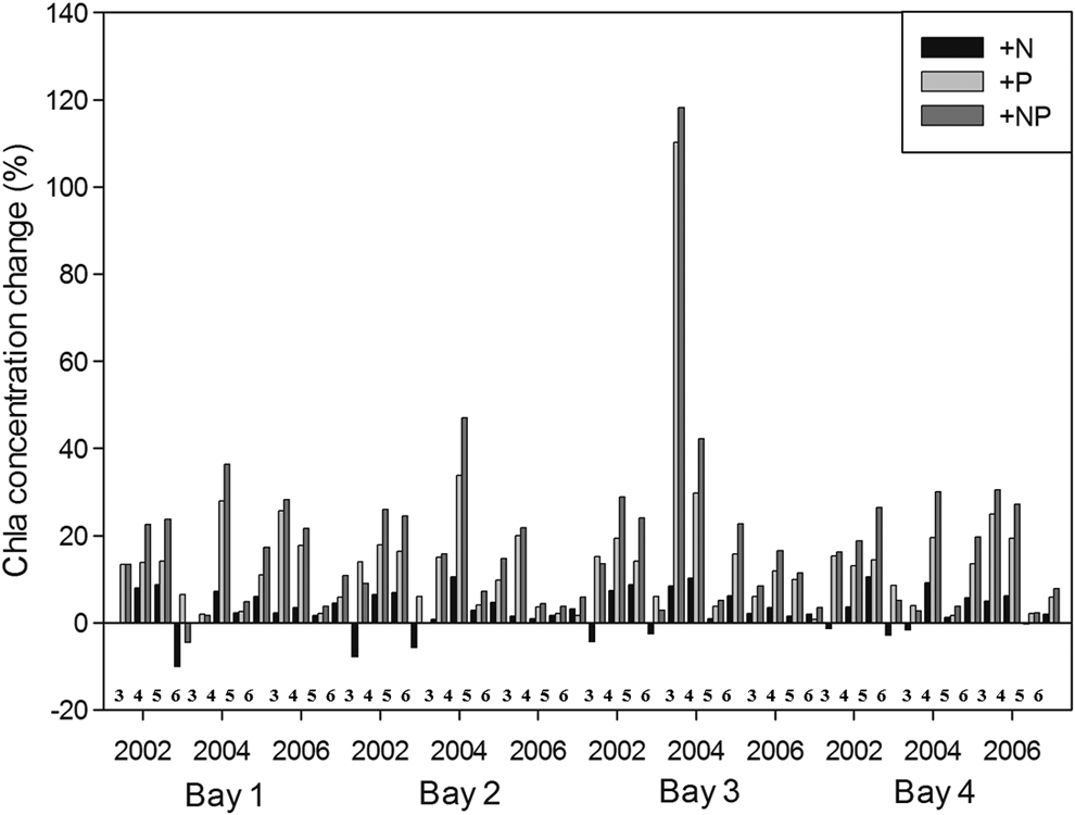
Change of chlorophyll-a concentrations from spring to early summer (March–June) in three simulations: (1) +N, (2) +P, and (3) +NP.

FIG. 8.

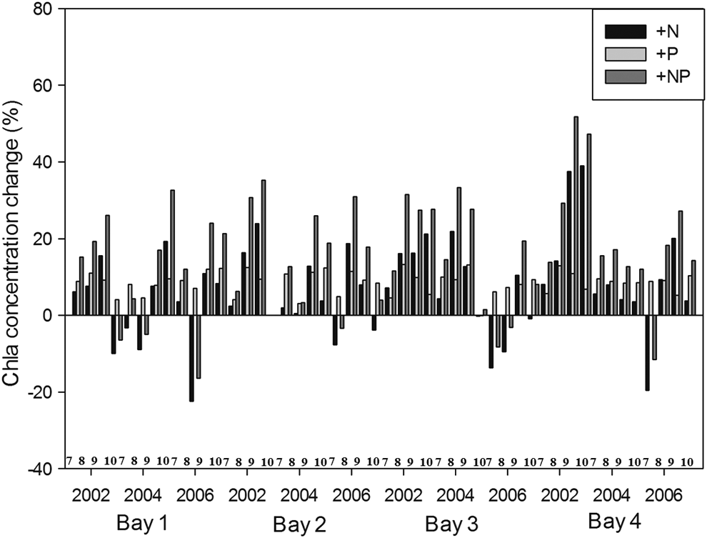
Change of chlorophyll-a concentrations from summer to fall (July–October) in three simulations: (1) +N, (2) +P, and (3) +NP.

Therefore, reducing P may no longer be adequate for Lake Taihu, and new nutrient reduction strategies should incorporate N-input reduction along with P-input reductions.

Conclusions

In this article, a BRBPNN model was created and used to predict the monthly chlorophyll-a concentration dynamics over a period of 15 years in Meiliang Bay, Lake Taihu. The following conclusions can be stated:

(a) The optimal network was found to consist of seven input neurons, six hidden neurons, and one output neuron. The coefficient of determination (R²) values (p < 0.001) for the training, validation, and test sets were 0.77, 0.49, and 0.76, respectively. The respective values of RMSE and bias for the three data sets are 17.24 and −1.05 for training, 12.48 and 0.62 for validation, and 11.01 and 2.2 for testing. The respective values of RMSE, bias, and the coefficient of determination (R²) for the four seasons are 14.31, 0.80, and 0.53 for spring, 22.10, −1.63, and 0.79 for summer, 12.35, 0.68, and 0.90 for fall, and 9.41, −0.1, and 0.38 for winter. Compared with MLR models, the BRBPNN model fits the data much better.

Thus, the BRBPNN model can be seen as a powerful tool for the prediction of long-term chlorophyll-a concentration dynamics in Meiliang Bay, Lake Taihu.

(b) Algae in the Meiliang Bay, principally Microcystis, were alkalophilic, and phytoplankton production was controlled by P inputs from spring to early summer, whereas N played a more dominant controlling role in summer–fall. Therefore, reducing P may no longer adequate for Lake Taihu, and new nutrient reduction strategies should incorporate N-input reduction along with P-input reductions.

Footnotes

Acknowledgments

This work was supported by the State Water Pollution Control and Treatment Technique Program of China (2013ZX07101014-05) and the Natural Science Foundation of Jiangsu Province (BK20140603). The Taihu laboratory for Lake Ecosystem Research (CNERN TaiLLER), Chinese Academy of Science, supplied the monitoring data.

Author Disclosure Statement

No competing financial interests exist.

References

Brewer

P.G.

, and Goldman

J.C.

(1976). Alkalinity changes generated by phytoplankton growth. Limnol. Oceanogr., 21, 108.

Bruder

, Babbar-Sebens

, Tedesco

, and Soyeux

(2014). Use of fuzzy logic models for prediction of taste and odor compounds in algal bloom-affected inland water bodies. Environ. Monit. Assess., 186, 1525.

Burden

F.R.

, and Winkler

D.A.

(2000). A quantitative structure-activity relationships model for the acute toxicity of substituted benzenes to Tetrahymena pyriformis using Bayesian-regularized neural networks. Chem. Res. Toxicol., 13, 436.

Chang

(1995). Major environmental changes since 1950 and the onset of accelerated eutrophication in Taihu Lake, China. Acta Palaeontol. Sin., 35, 155.

Chen

Y.W.

, Qin

B.Q.

, Teubner

, and Dokulil

M.T.

(2003). Long-term dynamics of phytoplankton assemblages: Microcystis-domination in Lake Taihu, a large shallow lake in China. J. Plankton Res., 25, 445.

Chenard

J.-F.

, and Caissie

(2008). Stream temperature modelling using artificial neural networks: Application on Catamaran Brook, New Brunswick, Canada. Hydrol. Process., 22, 3361.

Cho

, Lim

, Jung

, Kim

, Chae

, Park

, and Park

J.K.

(2014). Factors affecting algal blooms in a man-made lake and prediction using an artificial neural network. Measurement, 53, 224.

Coad

, Cathers

, Ball

J.E.

, and Kadluczka

(2014). Proactive management of estuarine algal blooms using an automated monitoring buoy coupled with an artificial neural network. Environ. Model. Softw., 61, 393.

Dokulil

M.T.

, and Teubner

(2000). Cyanobacterial dominance in lakes. Hydrobiologia, 438, 1.

10.

Duan

H.T.

, Ma

R.H.

, Xu

X.F.

, Kong

F.X.

, Zhang

S.X.

, Kong

W.J.

, Hao

J.Y.

, and Shang

L.L.

(2009). Two-decade reconstruction of algal blooms in China's Lake Taihu. Environ. Sci. Technol., 43, 3522.

11.

Foresee

F.D.

, and Hagan

M.T.

(1997). Gauss-Newton approximation to Bayesian learning. 1997 IEEE International Conference on Neural Networks, Huston, America, June 09–12.

12.

In Ieong

, Lou

, Ung

W.K.

, and Mok

K.M.

(2014). Using principle component regression, artificial neural network, and hybrid models for predicting phytoplankton abundance in Macau storage reservoir. Environ. Model. Assess., 20, 355.

13.

Khan

F.A.

, and Ansari

A.A.

(2005). Eutrophication: An ecological vision. Bot. Rev., 71, 449.

14.

Liu

, Lu

, and Chen

(2011). The effects of temperature and nutrient ratios on Microcystis blooms in Lake Taihu, China: An 11-year investigation. Harmful Algae, 10, 337.

15.

Liu

, Xi

D.G.

, and Li

Z.L.

(2015). Determination of the optimal training principle and input variables in artificial neural network model for the biweekly chlorophyll-a prediction: A case study of the Yuqiao Reservoir, China. PLoS One., 10, e0119082.

16.

Livingstone

D.J.

(2009). Artificial Neural Networks: Methods and Applications. Humana Press, New York, New York.

17.

Mackay

D.J.C.

(1992). Bayesian interpolation. Neural Comput., 4, 415.

18.

Maier

H.R.

, and Dandy

G.C.

(2001). Neural network based modelling of environmental variables: A systematic approach. Math. Comput. Model., 33, 669.

19.

Paerl

H.W.

, Gardner

W.S.

, McCarthy

M.J.

, Peierls

B.L.

, and Wilhelm

S.W.

(2014). Algal blooms: Noteworthy nitrogen. Science, 346, 175.

20.

Paerl

H.W.

, Xu

, Hall

N.S.

, Rossignol

K.L.

, Joyner

A.R.

, Zhu

, and Qin

(2015). Nutrient limitation dynamics examined on a multi-annual scale in Lake Taihu, China: Implications for controlling eutrophication and harmful algal blooms. J. Freshwater. Ecol., 30, 5.

21.

Paerl

H.W.

, Xu

, McCarthy

M.J.

, Zhu

G.W

, Qin

B.Q

, Li

Y.P

, and Gardner

W.S.

(2011). Controlling harmful cyanobacterial blooms in a hyper-eutrophic lake (Lake Taihu, China): The need for a dual nutrient (N & P) management strategy. Water Res., 45, 1973.

22.

Singh

K.P.

, Basant

, Malik

, and Jain

(2009). Artificial neural network modeling of the river water quality—A case study. Ecol. Model., 220, 888.

23.

Smith

V.H.

(2003). Eutrophication of freshwater and coastal marine ecosystems: A global problem. Environ. Sci. Pollut. Res. Int., 10, 126.

24.

Song

L.R.

, Chen

, Peng

, Wan

, Gan

N.Q.

, and Zhang

X.M.

(2007). Distribution and bioaccumulation of microcystins in water columns: A systematic investigation into the environmental fate and the risks associated with microcystins in Meiliang Bay, Lake Taihu. Water Res., 41, 2853.

25.

Tugcu

, Yilmaz

H.B.

, and Sacan

M.T.

(2014). Comparative performance of descriptors in a multiple linear and Kriging models: A case study on the acute toxicity of organic chemicals to algae. Environ. Sci. Pollut. R., 21, 11924.

26.

Vant

W.N.

, Hua

Y.Z.

, Jiang

Y.C.

, McBride

G.B.

, Roper

D.S.

, and Wang

(1998). Analysis of Lake Taihu eutrophication data 1989–1993. J. Lake Sci., 10 (Suppl), 143.

27.

Wei

, Sugiura

, and Maekawa

(2001). Use of artificial neural network in the prediction of algal blooms. Water Res., 35, 2022.

28.

N.C

, Huang

J.C

, Schmalz

, and Fohrer

(2013). Modeling daily chlorophyll a dynamics in a German lowland river using artificial neural networks and multiple linear regression approaches. Limnology, 15, 47.

29.

X.D.

, Kong

F.X.

, Chen

Y.W.

, Qian

, Zhang

L.J

, Yu

, Zhang

, and Xing

(2010). Horizontal distribution and transport processes of bloom-forming Microcystis in a large shallow lake (Taihu, China). Limnologica, 40, 8.

30.

, Paerl

H.W.

, Qin

B.Q.

, Zhu

G.W.

, and Gao

(2010). Nitrogen and phosphorus inputs control phytoplankton growth in eutrophic Lake Taihu, China. Limnol. Oceanogr., 55, 420.

31.

, Zeng

G.M.

, Xu

X.Y.

, Huang

G.H.

, Jiang

, and Sun

(2006). Application of Bayesian regularized BP neural network model for trend analysis, acidity and chemical composition of precipitation in North Carolina. Water Air. Soil Poll., 172, 167.

32.

, Huang

, Wei

Z.B.

, Luo

, Miao

A.J.

, and Yang

L.Y.

(2013). Seasonal variation of phytoplankton nutrient limitation in Lake Taihu, China: A monthly study from year 2011 to 2012. Ecotoxicol. Environ. Saf., 94, 190.

33.

, Shan

, Gao

H.L.

, Zhang

R.B.

, Wang

, and Qian

(2015). Long-term seasonal nutrient limiting patterns at Meiliang Bay in a large, shallow and subtropical Lake Taihu, China. J. Limnol. (AoP), 74, 519.

34.

Zhang

X.Q.

, Recknagel

, Chen

Q.W.

, Cao

H.Q.

, and Li

R.N.

(2015). Spatially-explicit modelling and forecasting of cyanobacteria growth in Lake Taihu by evolutionary computation. Ecol. Model., 306, 216.

Supplementary Material

Please find the following supplemental material available below.

For Open Access articles published under a Creative Commons License, all supplemental material carries the same license as the article it is associated with.

For non-Open Access articles published, all supplemental material carries a non-exclusive license, and permission requests for re-use of supplemental material or any part of supplemental material shall be sent directly to the copyright owner as specified in the copyright notice associated with the article.

0.00 MB

0.33 MB